On the study of genetic structure in human populations and the effects of demographic history, consanguinity, and study design on detection, with investigations of human evolutionary models, archaic introgression, and natural selection

Università degli Studi di Ferrara

DOTTORATO DI RICERCA IN

BIOLOGIA EVOLUTIONAISTICA E AMBIENTALE

CICLO XXIII°

COORDINATORE Prof. Guido Barbujani

ON THE STUDY OF GENETIC STRUCTURE IN HUMAN

POPULATIONS AND THE EFFECTS OF DEMOGRAPHIC HISTORY,

CONSANGUINITY, AND STUDY DESIGN ON DETECTION, WITH

INVESTIGATIONS OF HUMAN EVOLUTIONARY MODELS,

ARCHAIC INTROGRESSION, AND NATURAL SELECTION

Settore Scientifico Disciplinare BIO/18

Dottorando Tutore

Dott. Ferrucci Ronald Robert Prof. Barbujani Guido

_______________________________ _____________________________

(firma) (firma)

Università degli Studi di Ferrara

DOCTOR OF PHILOSOPHY IN

EVOLUTIONARY AND ENVIRONMENTAL BIOLOGY

23rd _CYCLE

COORDINATOR Prof. Guido Barbujani

ON THE STUDY OF GENETIC STRUCTURE IN HUMAN

POPULATIONS AND THE EFFECTS OF DEMOGRAPHIC HISTORY,

CONSANGUINITY, AND STUDY DESIGN ON DETECTION, WITH

INVESTIGATIONS OF HUMAN EVOLUTIONARY MODELS,

ARCHAIC INTROGRESSION, AND NATURAL SELECTION

Settore Scientifico Disciplinare BIO/18

PhD Student Tutor

Mr. Ronald R. Ferrucci Prof. Guido Barbujani

_______________________________ _____________________________

(firma) (firma)

Your E-Mail Address

ronald.ferrucci@gmail.com Subject

Genetics

Io sottoscritto Dott. (Cognome e Nome) Ferrucci Ronald Robert

nato a

New Haven, Connecticut, United States Provincia

Connecticut il giorno

8 January 1972

avendo frequentato il corso di Dottorato di Ricerca in: Evolutionary and Environmental Biology Ciclo di Dottorato

23

Titolo della tesi in Italiano

SULLO STUDIO DELLA STRUTTURA GENETICA DI POPOLAZIONI UMANE E LE EFFETTI DELLA STORIA DEMOGRAFICA, LA

CONSANGUINEITÀ, E DESIGN STUDIO SUL RILEVAMENTO, CON LE INDAGINI DI HUMAN EVOLUTIVA MODELS, ARCAICA

INTROGRESSIONE, E LA SELEZIONE NATURALE Titolo della tesi in Inglese

ON THE STUDY OF GENETIC STRUCTURE IN HUMAN

POPULATIONS AND THE EFFECTS OF DEMOGRAPHIC HISTORY, CONSANGUINITY, AND STUDY DESIGN ON DETECTION, WITH INVESTIGATIONS OF HUMAN EVOLUTIONARY MODELS, ARCHAIC INTROGRESSION, AND NATURAL SELECTION

Titolo della tesi in altra Lingua Straniera Tutore - Prof:

Guido Barbujani

Settore Scientifico Disciplinare (SSD) BIO/18

Parole chiave (max 10)

population genetics, evolution, Neanderthal, structure, CEPH HGDP, Cilento, genetic structure, conservation genetics, microsatellites, model-based

clustering Consapevole - Dichiara

CONSAPEVOLE --- 1) del fatto che in caso di dichiarazioni mendaci, oltre alle sanzioni previste dal codice penale e dalle Leggi speciali per l’ipotesi di falsità in atti ed uso di atti falsi, decade fin dall’inizio e senza necessità di alcuna formalità dai benefici conseguenti al provvedimento emanato sulla base di tali dichiarazioni; -- 2) dell’obbligo per l’Università di provvedere al

dall’Università di Ferrara ove si richiede che la tesi sia consegnata dal

dottorando in 4 copie di cui una in formato cartaceo e tre in formato .pdf, non modificabile su idonei supporti (CD-ROM, DVD) secondo le istruzioni pubblicate sul sito : http://www.unife.it/dottorati/dottorati.htm alla voce ESAME FINALE – disposizioni e modulistica; -- 4) del fatto che l’Università sulla base dei dati forniti, archivierà e renderà consultabile in rete il testo completo della tesi di dottorato di cui alla presente dichiarazione attraverso l’Archivio istituzionale ad accesso aperto “EPRINTS.unife.it” oltre che attraverso i Cataloghi delle Biblioteche Nazionali Centrali di Roma e Firenze. --- DICHIARO SOTTO LA MIA RESPONSABILITA' --- 1) che la copia della tesi depositata presso l’Università di Ferrara in formato cartaceo, è del tutto identica a quelle presentate in formato elettronico (CD-ROM, DVD), a quelle da inviare ai Commissari di esame finale e alla copia che produrrò in seduta d’esame finale. Di conseguenza va esclusa qualsiasi responsabilità dell’Ateneo stesso per quanto riguarda eventuali errori, imprecisioni o omissioni nei contenuti della tesi; -- 2) di prendere atto che la tesi in formato cartaceo è l’unica alla quale farà riferimento l’Università per rilasciare, a mia richiesta, la dichiarazione di conformità di eventuali copie; -- 3) che il

contenuto e l’organizzazione della tesi è opera originale da me realizzata e non compromette in alcun modo i diritti di terzi, ivi compresi quelli relativi alla sicurezza dei dati personali; che pertanto l’Università è in ogni caso esente da responsabilità di qualsivoglia natura civile, amministrativa o penale e sarà da me tenuta indenne da qualsiasi richiesta o rivendicazione da parte di terzi; -- 4) che la tesi di dottorato non è il risultato di attività rientranti nella normativa sulla proprietà industriale, non è stata prodotta nell’ambito di progetti finanziati da soggetti pubblici o privati con vincoli alla divulgazione dei risultati, non è oggetto di eventuali registrazioni di tipo brevettale o di tutela. --- PER ACCETTAZIONE DI QUANTO SOPRA RIPORTATO

Firma Dottorando

Ferrara, lì ___________________________

Firma del Dottorando _________________________________ Firma Tutore

Visto: Il Tutore Si approva Firma del Tutore ________________________________________

INDEX

1.1.6 Approaches to Studies of Genetic Structure . . . 19

1.2 Isolated Populations . . . 22

1.3 Study Design . . . 23

1.3.1 Scantily-Differentiated Populations . . . 23

1.3.2 Relatedness . . . 24

1.3.3 Effect of Marker Numbers on the Detection of Structure . . 25

1.3.4 SNP Markers and the Detection of Structure . . . 26

1.3.5 Effect of Marker Choice on the Detection of Structure . . . . 27

1.4 ALDH2 . . . 27

1.5 Models of Human Evolution . . . 28

1.6 Archaic Admixture . . . 30

1.7 Autocorrelation . . . 31

2 SCOPE OF THE THESIS 34 3 MATERIALS AND METHODS 36 3.1 Datasets . . . 36

3.1.1 Cilento . . . 36

3.1.2 CEPH HGDP . . . 36

3.1.4 Y-STRP data . . . 38

3.2 Genealogical analyses . . . 40

3.3 Simulation and Sampling Schemes . . . 41

3.3.1 Scantily-Differentiated Populations . . . 41

3.3.2 Family group analyses . . . 41

3.3.3 Marker Numbers . . . 41

3.4 Clustering analyses . . . 43

3.4.1 Comparison of Genealogical versus Genetic data . . . 43

3.4.2 Scantily-differentiated populations . . . 44

3.4.3 Consanguineous populations . . . 44

3.4.4 Marker Numbers . . . 44

3.5 Analytical Approaches . . . 46

3.5.1 Genealogical versus genetic data . . . 46

3.5.2 Scantily-differentiated Populations . . . 46

3.5.3 Marker Numbers . . . 47

3.6 Generalized Hierarchical Modeling . . . 47

3.7 Estimation of Demographic Parameters . . . 50

3.8 Archaic Admixture Simulation and Analysis . . . 54

3.9 ALDH2 Simulation and Analysis . . . 55

3.10 AIDA . . . 55

3.11 Correlation and Other Statistical Analyses . . . 58

4 RESULTS 59 4.1 Comparison of Genealogical and Genetic Data . . . 59

4.1.1 Genetic clustering . . . 59

4.1.2 Validation of genetic clustering using genealogical data . . . 61

4.1.3 Cluster Membership and Relatedness . . . 62

4.2 Scantily-differentiated populations . . . 64

4.2.1 Effect of Demographic Parameters on Clustering Methods . 64 4.2.2 Effect of Consanguinity on Clustering Methods . . . 65

4.3 Marker Numbers . . . 67

4.4 ALDH2 . . . 74

4.5 Archaic Admixture . . . 77

4.6 AIDA . . . 82

5 DISCUSSION 85 5.1 Comparison of Genetic and Genealogical Data . . . 85

5.2 Scantily-differentiated populations . . . 86

5.3 Marker Numbers . . . 88

5.4 ALDH2 . . . 92

5.5 Archaic Admixture . . . 92

1

Introduction

Charles Darwin ignited a revolution in biological thought with the publication of On the Origin of Species in 1859. The idea that plants and animals, as well as other life forms, were not fixed in form and had, in fact, evolved from common ancestors to fill various niches to which they were supremely adapted was a momentous one; one that would shake up the scientific world in the years to come. Though Darwin did not address human origins until publication of The Descent of Man in 1874, he portended what would come, writing that “[l]ight will be thrown on the origin of man and his history.” Just as Darwin’s book had earlier revolutionized biological thought, the advent of genetics and molecular technologies at the end of the last century has revolutionized research into human origins. Genetic studies have shown that humans share a common ancestor with chimpanzees, that all human populations are descended from an ancestral population in East Africa, and have enabled the reconstruction of a great deal of the evolutionary history of the human species.

One of the more prolific areas of recent research in human population genetics has been on the structure of human populations, which has seen great strides made in the last few years due to extensive collection of DNA samples from worldwide populations, both at the global [1,2], continental [3–5], and fine scale or geograph-ically limited [6, 7] levels, and from the generation of large amounts of data using high-throughput technologies [8–10]. Studies of genetic structure, the observation that populations are not genetically homogenous, are important in disease-gene association studies, conservation genetics, and anthropological research.

1.1

Genetic Variation

1.1.1 Genetic Structure

The study of genetic variation has done much to inform us of human origins and relationships. Furthermore, interest in studies of genetic variation have proven applicable to the medical field, particularly in association studies, where cryptic population structure may flummox attempts at discovering genetic variants asso-ciated with susceptibility to complex disease. Genetic structure is the observation that populations are not genetically homogenous, that is, that they can be divided,

genetically, into subpopulations or groups of subpopulations. This results when some sort of barrier (e.g., geographic, linguistic, cultural), or adequate distance, results in isolation between a set of populations [11]. Consequently, isolation cre-ates drift within populations, resulting in the differential distribution of alleles between and among populations, which, over time, results in differences in allele frequencies among them [12]. The subsequent divergence between populations is referred to as structure.

1.1.2 Genetic Drift

Genetic drift is a function of finite sampling: random gametes are sampled from a limited gene pool during reproduction to be represented in the next generation. As a result, some alleles tend to be overrepresented in different populations in the next generation, some underrepresented, and some may disappear completely. Over time, this continuous, cumulative random selection of gametes, known as genetic drift, results in differential distribution of alleles between and among populations, which is seen as differences in gene frequencies. Genetic drift, and thus genetic structure, is affected by a number of important evolutionary processes, including

effective size, divergence time, and gene flow. Effective size (Ne) refers to the

size (i.e., number of breeding individuals) of the optimum population showing allelic frequencies similar to the one being considered with the same degree of inbreeding, which is in Hardy-Weinberg equilibrium. Effective size is often smaller than census size. Decreasing the effective size within populations and increasing the divergence time between populations results in increased genetic drift within and between populations, thus resulting in greater genetic differentiation. To the contrary, gene flow counteracts the effect of drift by breaking down differentiation between populations, through transmission of new alleles into populations.

1.1.3 Coalescence

The coalescent is a stochastic process providing a backward-in-time approach for reconstructing the evolutionary history of a set of DNA sequences or genomes [13]. Going back in time, lineages are randomly chosen and merged at each generation until converging at the most recent common ancestor (MRCA) of all lineages [13]. Coalescent based simulations have proven useful in population genetic studies

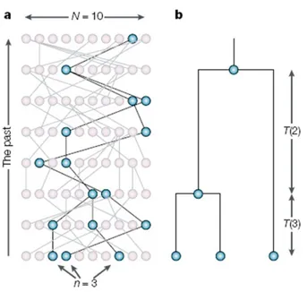
for their ability to reconstruct complex demographic scenarios, including bottle-necks, founder effects, and population fissions and fusions, among others. Their usefulness extends to testing hypotheses of human evolutionary models and differ-entiating natural selection from neutral evolution [13]. Figure 1 shows a sample coalescence for N=10 haploid individuals, without recombination or mutation. In the absence of recombination, coalescent history will often be constructed first and then mutations are placed along lineages descending from the MRCA. With recombination in coalescent simulations, lineages bifurcate as well as coalesce. As such, different pieces of DNA or different genomes will have slightly different topologies. Topologies are essentially phylogenetic representations of evolution-ary history. Thus, with recombination different evolutionevolution-ary histories result from different chromosomes or chromosomal pieces (see Figure 2). In a coalescent simu-lation, diploid individuals will be modeled following 2N haploid individuals. Prior to discovery of the coalescent, researchers used forward in time approaches, which were very time and computationally intensive. The Coalescent is more efficient because it only has to keep track of lineages that survive [13].

Figure 1: (a) Sample coalescent for 10 haploid individuals tracing back 8 generations.

The sub-genealogy for three single genomes that coalesce back to a single genome are shown in (b), with blacks lines showing the coalescent lineages. Coalescent times for the first and second coalescent events are indicated by T(3) and T(2), respectively [13].

Figure 2: (a) Coalescent history for 20 haploid individuals tracing back 17 generations, with (b) and (c) red lines showing the coalescent history for six individual genomes trac-ing back to a strac-ingle genome. (d) shows the coalescent history for a set of chromosomes with recombination [14].

1.1.4 Markers

Genetic variation is studied using a number of genetic markers located in non-coding (i.e., neutral) genomic regions. This is important because it ensures that differences in allele frequencies among populations are due solely to the effects of drift, mutation, and gene flow, and not to selective pressures. Single-nucleotide polymorphisms (SNPs) are markers that are based on variation in the state of nucleotides at a particular site and are often, though not always, biallelic. More than two states may exist, but it is the exception not the rule. With SNPs, there will often be a sequence of DNA that is mostly non-variant, that is, the DNA sequence at most sites is the same in all individuals. However, at certain sites, approximately once every 1500 nucleotides, there will be differences in the state of the nucleotide among individuals. Though often occurring in neutral areas of the genome, SNPs may also appear in genes and can affect regulation, if occurring in the promoter region, or protein structure, if appearing in exons. Microsatellites, or short tandem repeat polymorphisms (STRs or STRPs) are markers that show

variation in the number or length of repeats of a two to six letter motif. These often have higher mutation rates than SNPs, and are therefore useful in more recently diverged species or populations, such as in the human species. As such, they were the marker of choice for the CEPH HGDP [1, 2], as well as extensions of the panel in Native American [5], South Pacific [3], African [4], and South Asian populations [15]. SNP markers, however, are more amendable to high-throughput genotyping and have been the marker of choice for more recent analyses [6, 7, 10], including the CEPH HGDP [16]. A number of models of microsatellite mutation have been proposed. The more generally accepted one is the Single Stepwise Mutation Model (SSM, or SMM), where addition or deletion of repeats is expected to occur in single-steps [17]. Other models include a Generalized Stepwise Mutation Model, GSM [18], whereby addition or deletion of repeats may be more than one repeat according to a geometric probability distribution, and the Infinite Alleles Model (IAM), where any repeat number can change to any other repeat number. That is, any number of repeats may be added or deleted [19, 20]. The IAM is also the accepted mutational model for SNPs and genes.

1.1.5 Metrics

F-statistics. Wrights F-statistics [21] is one of the more widely used methods de-vised for analyses of population structure. F-statistics are measures of genetic vari-ation within and between populvari-ations and regions. Essentially, they describe the degree to which genetic variation amongst a set of populations may be attributed to variation within a local population (that is, between individuals within a local population), between populations within a region, and between regions. Another way to look at them is as a measure of correlation between alleles randomly cho-sen from one of these levels of apportionment [22]. One of the more widely used

measures is FST, which is the correlation between alleles chosen randomly from

within a subpopulation compared to the population as a whole [22]. It may also be seen as the proportion of genetic variation that is attributed to genetic differences between subpopulations [22]. As such, it may be used to measure differentia-tion between or among populadifferentia-tions, and can be considered a measure of genetic

distance between pairs of populations [22]. FST can be seen as a function of

effective population sizes decrease, genetic drift increases within populations, thus

increasing FST between and amongst them [11]. As well, reduced migration rates

also increase the effect of genetic drift, thus increasing FST. FST ranges from 0,

when subpopulations are completely identical, to 1, when all subpopulations are fixed for different alleles [11].

Gene Identity [23]. Gene identity is the probability that two randomly sampled copies of an allele, drawn from the same or different populations, are identical by state. Gene identity is also a measure of heterozygosity. As gene identity increases,

heterozygosity decreases, and vice versa. We refer to gene identity using the

notation Jk,l, where k = l indicates gene identity taken from within the same local

populations, and k 6= l indicates gene identity taken from between two different local populations. Gene identity is calculated from gene frequencies. If calculating gene identity from within the same local population, we use the equation,

Jk,k =

X

u

p2_ku

where pku is the frequency of the uth allele, with summation over all alleles.

Gene identity at a locus between two different local populations is calculated using the equation,

Jk,l =

X

u

pkuplu

where pku is the frequency of the uth allele in the kth population and plu is the

frequency of the uth _{allele in the l}th _{population. As above, summation occurs over}

all alleles. Other statistics, such as genetic distances or fixation indices, used in population genetic studies can be seen as functions of gene identities. As such, these statistics can be estimated from gene identities. However, the reverse is not necessarily true.

In analyses, it is helpful to organize sets of gene identities for pairs of popu-lations in a matrix, which we label J. Values on the diagonal correspond to gene identities within populations, while values on the off diagonal correspond to gene identities between populations. As long as populations in the matrix are orga-nized according to their tree of descent, gene identities in these matrices will take a block like pattern where populations sharing the same MRCA will be grouped

together. In addition, gene identity between a pair of population will be equal to the gene identity between their MRCA.

Kinship. Another way to measure relatedness between individuals is through coefficients of relatedness measuring the probability of identity by descent, such as estimated from pedigree data. This is usually seen as the proportion of an-cestry shared between pairs of individuals. There are a number of approaches for calculating kinship indices. The first, devised by Sewall Wright in 1922 [24], is the path counting approach, which traces all possible pathways shared by two individuals through common ancestors. Here, it is useful to think of relatedness between individuals as a set of loops connecting them through common relatives, and as a function of a hypothetical inbreeding coefficient in possible descendents, which we would determine using the equation

Φjk = Fi = (

1 2)

K

with Φjk being the kinship between individuals j and k, and Fi being the

inbreed-ing coefficient in their hypothetical offsprinbreed-ing, i, and where K is the number of ancestors in the loop connecting one allele in the “offspring” to the other. The calculation of kinship and inbreeding is additive across pathways. The coefficient of kinship is the probability that two individuals share alleles identical by descent, while the coefficient of inbreeding is the probability that two alleles within an individual are identical by descent. More recently, recursive approaches that are more computationally efficient have been devised [25] and implemented [26, 27], which are useful when considering large pedigrees.

Clusteredness. Model-based clustering programs output membership coeffi-cients that quantify a sample’s probability of belonging to a cluster or population (another way of looking at it, is as the proportion of ancestry from each cluster). These can be visually represented using a bar graph display as produced from the distruct program [28] or implemented in the gui version of structure [29]. Though this approach may be adequate when considering low numbers of experiments, a quantitative approach for summarizing the data is needed for large numbers of experiments. We chose clusteredness [30] as a metric for determining signifi-cant differentiation between populations. Essentially, clusteredness is the average membership coefficient for all sample individuals across all clusters, across all

in-dividuals, standardized by the number of clusters K, as per the following equation, G = 1 I I X i=1 v u u t K K − 1 K X k=1 (qik− 1/K)2

where I = number of individuals, K = number of clusters, and qik = the

mem-bership coefficient of the ith individual to the kth cluster. Standardizing by the

number of clusters is important because it allows for comparison across different numbers of K and is more intuitive to understand. Instead of average member-ship coefficients running from 1/K, as an indication of no clustering, to 1.0, as an indication of complete clustering, G runs from 0.0 to 1.0. Thus, also, one can easily identify a minimum clusteredness as indicative of structure that applies to all levels of K. For example, 0.5 corresponds to an average membership coefficient of 0.75 (or 0.9, to 0.95).

Symmetric Similarity Coefficient. Model-based clustering algorithms may some-times produce different outputs from the same data when using different starting points (i.e., different random numbers). It is useful to consider the similarity between runs to determine whether results are reliable. The following equation, implemented in the clumpp software, has been devised for quantifying the extent of similarity between pairs of runs,

SCC(Qi, Qj) = 1 −

min kQi− P (QjkF

pkQi− SkFkQj − SkF

where Qi and Qj are I x K matrices of membership coefficients for runs i and j

and, with columns (K ) corresponding to clusters and rows (I ) corresponding to individuals [31]. Each element is the membership coefficient of each individual to each cluster. P is a permutation of the columns, with the minimum taken over all permutations, for K permutations. F is the Frobenius matrix norm and S is a probability matrix of K = (number of clusters) columns, with all elements = 1/K [2, 31]. Use of this equation assumes that comparisons are across runs that have the same number of clusters, i. Rosenberg et al. [2], supplemental materials, provides suggestions for the interpretation of results: values of 0.85-1.00, nearly all individuals have nearly identical membership coefficients between runs; 0.4-0.85, most, but not all, individuals have nearly identical membership coefficients between runs; 0.1-0.4, some clusters have the same individuals but other clusters

differ between runs; and <0.1, little to no similarities between clusters.

Genetic Distance. Another measure of difference between populations is ge-netic distance, such as Nei’s minimum gege-netic distance. Nei’s distance measure is a function of allele frequencies and can be calculated from the gene identity within and between local populations using the equation,

D2_kl=X(pki− pli)2 = Jkk+ Jll− 2Jkl

where pki and pli are the ith allele frequencies in the kth and lth populations,

respectively, and Jkk, Jll, are gene identities within the kth and lth populations,

respectively, and Jkl, between the kth and lth populations.

1.1.6 Approaches to Studies of Genetic Structure

Traditional. Traditional approaches to the study of genetic structure often involve apportioning genetic variation into three categories: between individuals within local populations, between populations within a specific region or grouping, and between regions (or other grouping) within the dataset as a whole. The proportion of variation attributed to each category gives an indication of the genetic structure between populations [12]. A similar approach, termed Analysis of Molecular Vari-ance (AMOVA), essentially an extension of ANOVA, was proposed for analysis of molecular data [32]. AMOVA has given some statistical standing to the study of genetic apportioning by providing a method for determining significance. Most estimates of genetic structure in human populations provide that 85% of genetic variation is found within a population, with 15% left between populations, either within the region or between regions [12]. The traditional approach contains an inherent flaw in that it assumes division of populations neatly into regions, and without regard to evolutionary or demographic history. As Long et al. [33] show, discrete compartmentalization of human populations may be flawed in light of human evolutionary history.

Model-Based Clustering. The development of model-based clustering methods in recent years has revolutionized the study of genetic structure in human popu-lations. Previously, analyses of genetic structure required pre-defined assignment of samples into populations. This required the assumption that populations from which individuals were sampled correspond to the actual population from which

they originated. While this may sometimes be a valid assumption, particularly in the case of isolated populations, large increases in migration between popu-lations have occurred over the last 100 years, even in isolated popupopu-lations (i.e., breakdown of isolates [34]). In our own sample populations from southern Italy, we have found evidence of individuals being sampled from populations other than the one into they were born. This was evidenced through comparison with par-ents, or other relative, that were also sampled in our study. Also, some sample individuals are descended from parents from two populations. Model-based clus-tering approaches allow researchers to overcome limitations such as these by using Bayesian [35], expectation-maximization [36], or maximum likelihood [37] methods to determine the optimum distribution of sample individuals into a set of clusters based on statistically optimized allele frequency distributions. In addition, these methods can also group populations with other populations to which they are more closely aligned genetically and, in the presence of admixture can determine the probability of an individual belonging to a cluster or the proportion of their genome having membership to a cluster.

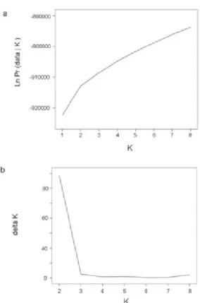
In addition, output from model-based clustering programs, such as structure [35], can help to identify the most likely number of clusters in the sample. One may use the original approach suggested by Jonathan Pritchard of analyzing posterior priors output by his program, structure, for a set of K number of clusters, from 1, 2, 3,. . . ,N, with N being the maximum number of clusters estimated [29]. However, this approach sometimes fails to provide a definitive answer. Another approach, suggested by Evanno [38], looks at the change in log likelihood as a guide. Finally, an additional ad hoc approach more recently suggested by Pritchard is to examine the membership coefficients estimated for the samples [29]. When individuals have a tendency to be placed into a single cluster as opposed to being distributed across a number of clusters, this may be considered to be the correct K.

The structure algorithm is a Markov Chain Monte Carlo method, which uses burnin length and number of iterations following burnin to minimize the effect of the starting configuration and optimize estimation of parameters, respectively [29]. Burnin length and iterations following burnin are determined by the user. Adequate length of burnin and number of iterations following burnin are important in ensuring convergence of the MCMC chain [29]. These should be chosen so that parameters converge, that is, reach an equilibrium, before data is collected.

Generalized Hierarchical Modeling [23]. While clustering populations using model-based clustering programs can be useful for identifying clusters of closely-related populations, cryptic population structure, and inter-individual closely-relatedness, it may be useful to turn to other methods to test hypotheses on population struc-ture and relatedness, methods that allow testing of complex scenarios of strucstruc-ture. One such method is generalized hierarchical modeling (ghm), which may also be termed generalized analyses of molecular variance, which provides for a structured approach to testing hypotheses. Generalized hierarchical modeling uses a system of equations developed by Anderson to fit models to data [39]. Application of these systems of equations to genetic data were first adapted by Cavalli-Sforza and Piazza in 1975 [40]. Models may include simple models, such as an island model, whereby all populations originate from a single ancestral population at one time and evolve independently, or more complex hierarchical models, whereby each population or set of populations branches off from earlier populations. The former model may also be called an independent regions model, while the latter models may also be called, and more easily-understood as, ‘nested’ models. These hierarchical models are assumed to be strictly nested, where the previous entry is a superset and the next entry is a subset [41].

While fitting models to the data, ghm estimates two sets of the researchers chosen metric, gene identity for example, for each model to be evaluated: expected and realized. Realized gene identities are probably the most intuitive, they are gene identities as measured from the data without regard to a particular model. We may also call them raw gene identities. Expected gene identities are those estimated from a given hierarchical model fitted to the gene identity matrix. To test the fit of models, we use a likelihood ratio statistic, Cavalli-Sforza and Piazza’s treeness statistic

Λ0Ω= v · (ln|det( ˆΣ0| − ln|det( ˆJ | + tr ˆJ ˆΣ−10 − r)

which is distributed as a χ2 statistic with degrees of freedoms equal to (r(r + 1)/2)

minus the number of parameters needed to fit the tree, where r is the number of populations, to determine the fit of the model to the data. v is the number of independent observations. An observation is an allele at a locus, and the number of independent observations is equal to (number of alleles at all loci - number of

loci - 1). This factor is most appropriate when allele frequencies are equal for each marker. Ongoing research hints that a more appropriate determinant for independent observations, when this requirement does not hold, is the number of effective alleles. The number of effective alleles is the inverse of the homozygosity, subtracting one and multiplying by the number of loci. In any case, the treeness statistic is still useful for testing the fit of a model and comparing the fit between

models. Models can be ranked by their χ2 values, with lower values corresponding

to better fitting models [42]. ˆΣ0 is the matrix of expected gene identities

deter-mined by the model and ˆJ is the matrix of observed gene identities. If the model

fits perfectly, that is, if the observed and expected gene identities differ by no more than would be expected from genetic and statistical sampling, Λ will be equal to the number of degrees of freedom [42]. Oftentimes, researchers will want to test different models to determine which one fits the data the best. These may begin as a parameter rich model that is subsequently reduced, as parameter poor models to which higher level groupings are subsequently added, or as models with differ-ent hierarchical structures that are independdiffer-ent of one another (such as models of Native American language evolution, see [42]).

1.2

Isolated Populations

Due to their expected genetic homogeneity and common environmental back-ground, resulting from isolation, geographical isolates are prime subjects for inves-tigating complex genetic traits and identifying common alleles involved in suscep-tibility to complex diseases [43–46]. However, even in populations considered to be particularly homogenous [47], the presence of undetected population stratifica-tion may result in the presence of groups of closely-related individuals, considered to be a major confounding factor in disease-gene association studies [48–50]. Un-fortunately, lacking reconstruction of genealogical relationships, detection of pop-ulation stratification, from the presence of inter-individual relatedness or cryptic structure, is most difficult [51,52]. Most reconstructed pedigrees have been limited in completeness, spanning at most a few generations. As such, researchers must rely on indirect evidence of genealogical relatedness, such as through studies of genetic variation. We felt it fruitful, therefore, to explore comparisons between genetic and genealogical data.

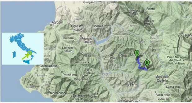
For isolated populations, in our work we used a set of closely-related popu-lations from the Cilento National Park in southern Italy, Gioi and Cardile (Fig-ure 3). Historical sources document that the village of Gioi was settled first in the

9th century by Greek immigrants, with a secondary settling of Cardile in the 18th

century through an exodus of Gioi residents. Though located approximately 6 km apart, the villages of Gioi and Cardile experienced high levels of reproductive

isolation until the 20th century. As in the case of many isolated villages around

Europe, a breakdown of isolates occurred following World War II that saw large scale migration from the Cilento region.

Figure 3: Map showing location of Gioi and Cardile within the Cilento National Park

in southern Italy.

1.3

Study Design

1.3.1 Scantily-Differentiated Populations

Bayesian clustering algorithms have shown to be effective at identifying genetic clusters in human populations [35, 36, 53]. Detection of differentiation and cluster-ing with these methods may be affected by a number of factors, such as number of markers considered and sample sizes [30, 54], mutation rate [55], and geographical dispersal of sample populations [30, 56]. The usefulness of model-based cluster-ing methods in describcluster-ing genetic structure has been demonstrated in studies

of globally-distributed, genetically well-differentiated populations [2, 30, 54], as well as in more closely-related, geographically-limited, but still genetically well-differentiated [3–5], ones. However, their efficacy in highly closely-related, scantily-differentiated populations has been limited to few studies involving real popula-tions [6, 57], or to simulapopula-tions of scantily-differentiated populapopula-tions [58]. Nearly all other previous studies have concentrated on populations among which genetic differences are substantial. As such, their efficacy for the analysis of scantily-differentiated populations is still an open question.

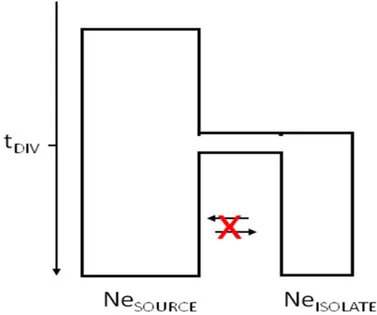
We used simulations to study the behavior of structure, one of the more exten-sively used programs, in the presence of limited genetic differentiation. Here, we varied effective size and divergence times, along with differences in sample sizes and markers numbers. See Figure 4 for our model.

Figure 4: Diagram of model showing isolated population diverging from its original

source population.

1.3.2 Relatedness

Increased consanguinity is common in scantily-differentiated populations. Though considered to be an important factor influencing inferences of genetic structure [59], the effect of related individuals on the performance of model-based clustering methods is not well documented, regardless of the existence of methods for esti-mation [60,61]. In fact, a number of studies in human populations have taken care to avoid including related individuals in order to limit the potential confounding

effect of consanguinity [4, 5, 15, 62]. However, the performance of model-based clustering methods, and the effects of study design, is largely unknown for con-sanguineous populations. To the best of our knowledge, the only other study to investigate the effect of consanguinity on clustering analyses was in rainbow trout, a species that differs from human populations in being polyandrous, and showing high fecundity and variance in reproductive success [63]. Further, their study consisted of a single-family group consisting of siblings and half siblings plus otherwise completely unrelated, or at least not obviously related, individuals, and their simulations modeled similarly structured populations, rather than a number of groups of related individuals with complex networks and varying degrees of relatedness that we see in human populations. Here, we test model-based clus-tering approaches in a set of consanguineous populations controlling for different levels of relatedness. We make use of an extensive genealogical dataset dating back three centuries to reconstruct genealogical links between sample individuals. In this part of the study, we identified and removed consanguineous individuals to investigate the effect of reducing relatedness in a sample on the performance of structure.

1.3.3 Effect of Marker Numbers on the Detection of Structure

While the study by Vitart [57] showed differentiation amongst closely-related pop-ulations among the Dalmatian islands, the observation of differentiation is weak

and mainly between villages that have approximately 0.02 or greater FST (paired

villages with lower FST values tend to cluster with other populations and do not

differentiate separately). Appropriately, Latch [58] showed that population

iden-tification by Bayesian methods breaks down amongst populations with FST below

0.02. However, conclusions from both these studies were based on just a handful of markers—26 in the former and 10 in the latter—, which we have found may be too low to detect clustering in scantily-differentiated populations. Analyses

of European populations, a lowly-differentiated group of populations with FST

<0.007 [2] documents a recognizable structure with 377 markers [2]. One may conclude, therefore, that it is difficult to judge whether failure to identify struc-ture in scantily-differentiated populations is due to either the prevalence of the effects of gene flow over those of genetic drift, or to an inadequate number of

markers in the analysis. However, even rather large numbers of markers may not necessarily be adequate, as in the case of linguistically-differentiated populations in India [15].

The question thus remains, is there a specific lower level of differentiation be-yond which, barring highly related populations, genetic structure is undetectable through model-based clustering methods? Or, is the detection of structure with

different levels of FST dependent on the number of markers available? Essentially,

would increasing the number of markers analyzed increase the possibility of ob-serving structure in populations with lower differentiation? Bamshad et al. [54] shows that the accuracy at which structure infers group membership for large-scale (i.e., continental or geographical) groupings is indeed affected by marker numbers, whereby increasing the numbers of markers analyzed increases correct predictions of individuals into their sampled continental populations. Further, Rosenberg et al. [30] shows a marker number effect on clusteredness, that is, the degree to which populations cluster with one specific group, which we may also refer to as the ability to detect structure, and demonstrated a contribution of marker numbers to clustering success in the case of chicken breeds [64].

Recently, Morin [65] showed that the power to detect structure increases with increasing number of markers analyzed in a data set, and that this observation

was affected by differentiation level. Both moderately (FST = 0.01) and scantily

differentiated populations (FST = 0.0025) show increasing power up to 75 markers.

However, high FST populations achieve high power approaching 75 markers (power

>0.9), while low FST populations do not even reach 50%. Increasing the number of

SNPs analyzed might have increased the observed power in scantily differentiated populations. These authors also show that minor allele frequencies seem to have no effect on results, indicating that SNP choice is not an issue. Although the marker system studied here were SNPs, we expect a similar relationship with microsatellites, our marker system of choice.

1.3.4 SNP Markers and the Detection of Structure

We focus on microsatellites in this study, as they have been one of the most com-monly used markers systems, and are more useful in relatively recently diverged populations (i.e., most human populations) because of their higher mutation rate.

However, it may also be of interest to ask how marker choice affects our ability to detect structure considering different numbers of markers. Lao et al. [8] suggests that more STRP than SNP markers would be needed for detection of population structure because of their high mutation rate. However, this is counter-intuitive; one would assume that given the low mutation rate of SNPs, STRPs would be more advantageous given the recent separation and shared ancestry of human populations (particularly for closely-related populations). In fact, STRPs have historically been used in studies of closely related populations because of their high mutation rate and high degree of variability. Though, Lao et al. [8] was referring to the case of using carefully ascertained SNPs.

1.3.5 Effect of Marker Choice on the Detection of Structure

Finally, Rosenberg et al. [66] showed that choice of markers, that is, choosing markers that are more informative, can affect identification of population clus-tering, whereby datasets of markers chosen to be informative are more useful in identifying genetic structure than are datasets of randomly chosen markers, reduc-ing the numbers of markers needed for structure analyses. As an aside, it would be of interest to know whether informativeness of markers influences the ability to detect differentiation between pairs of populations.

1.4

ALDH2

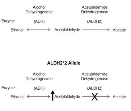
Acetaldehyde dehydrogenase 2 (ALDH2) is an enzyme involved in the alcohol metabolism pathway, specifically converting acetaldehyde to acetate (see Figure 5, top). A broken copy of the gene (see Figure 5, bottom), referred to as ALDH2*2, has been identified that causes accumulation of acetaldehyde in carriers [67], re-sulting in a flushing reaction in the face [68]. In addition to this flushing reac-tion, which may reduce alcoholism because of its unpleasantness, accumulation of acetaldehyde is also toxic and carcinogenic [69]. As a dominant acting allele het-erozygotes are also affected. Interestingly, this allele is found only in East Asian populations, and is a common allele in those populations [70]. We concern our-selves that this allele may have been the subject of recent selection on the East Asian branch. First, the high frequency of the allele indicates that it would have to be an old allele, but old alleles tend to be more dispersed globally, and second,

the negative effect of the allele would imply some counter advantage to it. Further, genetic loci that are common in one population tend to also be found dispersed amongst populations either because they are shared by descent or because they are transferred between populations through gene flow. In addition, a second allele is found only in populations on the OOA branch. Here, we explore the evidence for natural selection of ALDH2*2 through simulation of genes with features similar to ALDH2, comparing the distribution of alleles with frequencies similar to those observed in ALDH2*2 and the OOA limited allele.

Figure 5: Ethanol metabolism pathway, showing the breakdown of ethanol to acetate,

through an acetylaldehyde intermediate (top). The ALDH2*2 allele causes the accumu-lation of acetylaldehyde (bottom).

1.5

Models of Human Evolution

A number of models of human origins and evolutionary have been presented. These can easily be tested against predictions of gene identity patterns.

Independent Regions. Under the independent regions model, a set of modern human populations split from a single ancestral population, with little to no subse-quent gene flow between or among them, allowing them to evolve independently of

one another. This is analogous to the multi-regional model of human origins, but with modern human populations splitting from an ancestral modern population rather than an ancestral archaic population. This may also be referred to as an is-land model. We can also consider a nested independent regions model, where each geographical region splits from a single ancestral population, and all populations within the geographical region originate from that geographical population.This model predicts highest gene identities within local populations, lower ones be-tween populations within geographical regions, and lowest bebe-tween populations in different regions. Human genetic variation has been shown to be inconsistent with the independent regions model [71].

Isolation by distance. Isolation by distance is a function of the interacting ef-fects of drift and long-term gene flow with neighboring populations [11]. This occurs when individuals have greater likelihood of mating with individuals in neighboring populations than they do with ones located father away and results in individuals having a greater probability of sharing relatives in neighboring popu-lations and lower probability with popupopu-lations located at greater distances, which can be seen as a gradual decline in genetic relatedness with distance. Under this model, we expect declining gene identities with geographical distance between populations. Human genetic variation has been shown to be consistent with a model of long-range and local gene flow amongst Eurasian populations [71].

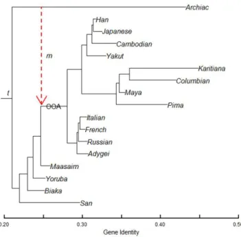
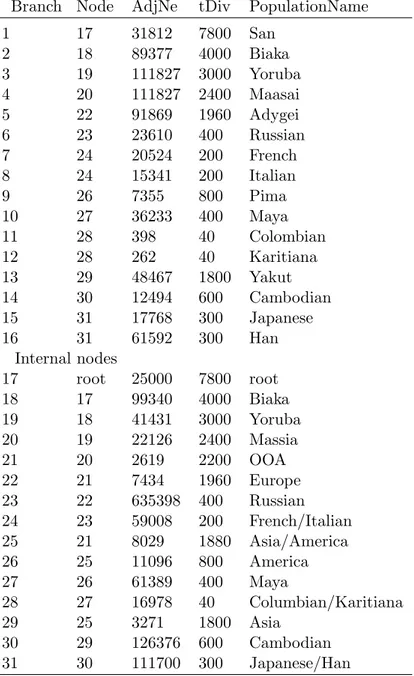
Serial Founder Effects. Previous studies have shown human genetic diversity to be consistent with a serial founder effects (SFE ) model [72]. Under the se-rial founder effects model, we see a set of population fissions, whereby each new population originates from a previous founding population and subsequently gives rise to future populations. However, subsequent investigations show that human genetic variation is better explained by a nested version of SFE model, where a series of major founder effects marked by bottlenecks occurs in major geographical regions, followed by a series of founder effects within regions [71]. Under the serial founder effects model, we expect to see: 1) lowest gene identities in the original, ancestral population (essentially, the root of the tree), 2) a sequential increase in gene identities between regions with each subsequent founder population, 3) a layered pattern of gene identity variation between regions and between popula-tions within regions [71], and 4) equal or similar gene identity between all pairs of populations that share the same MRCA. In addition, we expect a tree of descent

according to the pattern of fissions and length of branches on the tree that are proportional to the ratio of evolutionary time to effective size.

Though testing of hierarchical models show that human genetic variation is, generally, consistent with predictions from the SFE model, there are still some de-viations from the model that need to be accounted for. Specifically, non-African populations show greater diversity than expected under the SFE, resulting in greater than expected genetic distances between African and non-African popula-tions. We predict that early modern humans leaving Africa interbred and admixed with archaic populations that they encountered along the way, and that this in-jection of new genetic variants resulted in the increased variation that we observe.

1.6

Archaic Admixture

One of the most fundamental and contentious issues in human evolutionary studies has been the conflict between competing models of human origin. For years, the two reigning theories have been Multiregional Evolution (MRE) and the Out-of-Africa (OOA), or replacement, theories [73]. The MRE states that modern Homo sapiens originated, from early hominids, separately in Europe, Africa, and Asia and evolved independently in these regions, with subsequent gene flow between regional populations [74]. In contrast to the MRE, the OOA theory posits that all modern humans evolved from a single population in Africa, approximately 200,000 years ago, and then replaced existing Homo species in the rest of the Old World as they left Africa [75]. Much of the genetic evidence has favored the OOA theory to the detriment of the MRE theory. However, other theories, compromises between MRE and OOA, have been presented in recent years. Many of these new ideas are modified versions of OOA, with allowance for admixture [76]. Thus, the question being asked now is not whether humans originated in one location (OOA) or independently in the three main regions of the old world separately (MRE), but whether there was admixture between the population of modern humans leaving Africa 60,000 years ago and populations of archaic humans that they encountered along the way.

Studies of Neanderthal mitochondrial DNA (mtDNA) unequivocally show no evidence of admixture with modern humans [56, 77]. Comparisons of mtDNA se-quences between modern human and Neanderthal mtDNA sese-quences showed that

the genetic differences between Neanderthal and current modern humans were significantly different than that between current modern human populations such that there could have been no admixture [77]. Further, a comparison of Nean-derthal and early modern human sequences found that the early modern human mitochondria contained zero Neanderthal-like DNA [56]. Finally, mtDNA from Cro-magnon fossils shows variation within the range of current modern humans but distinct from that of Neanderthals [78]. Recent simulations also support an African replacement model for human evolution [79].

However, mitochondrial DNA is only one locus, and therefore can only tell part of the story [80]. If gene flow from Neanderthals into early modern humans were purely paternal, it would not leave a signature on mtDNA. Further, even if gene flow from Neanderthal were maternal, genetic drift could have removed all trace of admixture from the mitochondrial portion of the human genome [81]. In addition, we may expect that given the high mutation rate of mtDNA and length of time since possible admixture events, mutation could have erased signals of admixture as well. Of course, any possible signature on the modern human genome would be dependent on the admixture rate [82]. If Neanderthals made a tiny genetic contribution, there is a greater chance that those genes would be lost through drift. Estimates of rates of admixture range from 15 [83, 84] to 25% [56], to less than 0.1% [85]. Thus, if admixture rates were on the low end of the estimated admixture spectrum (i.e., <0.1%), it is not likely that we would see its signature in the modern human genome.

Recent technological advances have allowed amplification and sequencing of Neanderthal autosomal DNA, analyses of which, in comparison with modern man DNA, have revealed evidence of admixture between archaic and modern hu-mans [86]. Here, we show that evidence for archaic admixture with early modern humans can be detected in modern human genomic diversity, which may explain deviations from the SFE model.

1.7

Autocorrelation

Analyses of spatial autocorrelation, the dependence of values of a variable with values at different, usually adjoining, locations [87], are informative of demographic and evolutionary processes. Initially conceived by geographers and statisticians,

spatial autocorrelation methods were readily adopted by biologists for the study of genetic [88], morphometric [89], and ecological data [90]. However, the usage of spatial autocorrelation was limited to allele frequencies of individual markers or polymorphisms. Subsequently, Bertorelle and Barbujani [91] further adapted these methods for use with molecular data, such as DNA sequences, which they termed Autocorrelation Indices for DNA Analysis or AIDA. AIDA statistics II and cc, modified forms of the spatial autocorrelation indices Moran’s I and Geary’s c, respectively, measure sequence or haplotype similarity with distance [92]. Non-AIDA spatial autocorrelation analyses for the study of genetic variation has been likened a multivariable approach, because results from multiple analyses were often compared, in contrast to multivariate approaches such as principal components analysis (PCA) [93]; thus, AIDA can be viewed as an approach transforming spatial autocorrelation analysis from a multivariable to a multivariate approach.

Demographic and evolutionary processes, such as genetic drift, gene flow, and natural selection affect genetic variation generated by the action of mutation. While the effects of selection may sometimes be of interest to researchers, it is the patterns created by the opposing forces of drift and gene flow that are of interest in the case of spatial autocorrelation analyses. While genetic variation between and among populations is often thought of in discrete terms, and in fact genetic variation may be observed as discontinuous and can therefore be studied as such [35, 94], differences between and among populations may sometimes be more subtle, exhibiting clinal or continuous, often geographically-based, variation [87, 95]. Further, some evolutionary processes, such as isolation by distance, may require approaches that take into account subtle genetic variation, methods that do not require populations to be measured as completely distinct entities. Methods such as spatial autocorrelation are useful in this regard. Indeed, since not all genetic variation is discontinuous it would be inappropriate to treat all data as such. In addition, while clinal patterns of variation are easily observed by locating gene or haplotype frequencies on a map (using some graphical visualization), the statistical significance of these patterns may be open to question. Autocorrelation analyses may add statistical weight to these observed patterns.

In human populations, AIDA statistics have been mainly used to study Y-chromosome single-nucleotide polymorphisms [96–103] and mtDNA [77, 92, 104– 107] data. In addition, limited usage has been done on X-chromosomal data [108]

and coding sequences [109].

While an independent extension to AIDA for microsatellite data has been available for a number of years [110], autocorrelation analyses on microsatellites in humans have been limited to a few studies, using alleles at single markers [111], haplotype frequencies associated with single, specific haplogroups [112], or individual loci separately with AIDA [113], or haplogroups with [114] or without [115] AIDA. As such, the full power of genetic variability associated with the rapid mutation rate of Y chromosome microsatellites has not yet been realized. During our recent update of AIDA into the python programming language, which was done to increase the computational limit of AIDA (i.e., to free AIDA from limitations on number and length of sequences associated with previous versions), we decided to incorporate an option for microsatellite analyses into the new version. Along with this decision, it was determined that autocorrelation analyses of Y-chromosome microsatellites in European, both continental and regional, populations was long overdue. This also allowed us to test our new version.

2

SCOPE OF THE THESIS

a) To show that genealogical relationships within and between populations are expressed in genetic data

b) To show how demographic history can affect the detection of clustering in scantily-differentiated populations

c) To show how consanguinity affects the signal of structure in closely-related populations

d) To show that the detection of differentiation between pairs of populations is dependent on sample size and marker numbers considered

e) To show that the number of markers needed to identify differentiation between pairs of populations is dependent on their level of divergence

f) To develop a new version of AIDA with increased computational power and extended use for analyzing microsatellites

g) To show that modern human genetic variation is consistent with a serial founder effect model, long-range gene flow between populations in different regions of Eurasia, and introgression of archaic DNA into modern humans on the OOA branch

h) To show that the limited distribution of a detrimental allele in Asian populations is not consistent with neutral expectations

3

MATERIALS AND METHODS

3.1

Datasets

3.1.1 Cilento

From southern Italy, we have data available on 1356 individuals from two villages, Gioi (n = 882) and Cardile (n = 474), corresponding to nearly all current resi-dents, located within the Cilento National Park. Two sets of data were collected for these samples: genealogical and genetic. Our genealogical data is composed of 20,383 birth records, also documenting mortality and parental relationships, spanning the past four centuries, collected from registry office and parish archives. These data allowed us to reconstruct genealogical relationships between all pairs of extant individuals. For genetic data, we obtained 1122 microsatellites, with average marker spacing of 3.6 cM and mean marker heterozygosity of 0.70, from a genome-wide scan performed by the DeCode genotyping service on DNA extracted from peripheral blood. Genetic data was obtained from all study samples.

3.1.2 CEPH HGDP

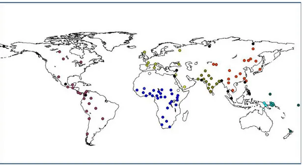
Our primary dataset of worldwide populations is the CEPH Human Genome Di-versity Panel (HGDP), which was initially a set of 1050 individuals distributed amongst 52 world-wide populations [1, 2] originally typed on 377 microsatellites, and subsequently extended to 783 microsatellites [30]. Subsequently, additional samples and populations have been typed for many of these same markers in Native American [5], South Asian [15], African [4], and South Pacific [3] popula-tions. We term this the ‘extended’ CEPH HGDP (see Figure 6 for locations of populations, black dots correspond to waypoints). This dataset contains 5179 in-dividuals from 245 populations genotyped at 619 common microsatellite markers. The original CEPH populations have also been typed for SNP markers [116]. For our first project using the Cilento populations, comparing results from genealog-ical and genetic analyses, we use European populations from the original CEPH HGDP dataset, using a subset of 36 markers shared between that dataset and our populations from Cilento. For the ALDH2 project, we use 16 populations from the original CEPH dataset. For our project analyzing marker numbers needed

to observe differentiation between populations with different levels of divergence, we use the Wang et al. [5] dataset of original CEPH data plus additional Na-tive American populations. For the archaic admixture project, we use subsamples taken from the ‘extended’ CEPH HGDP. Geographical distances between popu-lations are great circle distances calculated using the indicated waypoints taking into account inferred directions of dispersal across land.

Figure 6: Map of world with locations of populations from extended CEPH HGDP.

Black dots indicate waypoints.

3.1.3 ALDH2

We obtained DNA samples from four populations each from four geographical re-gions: Africa (Mbuti, 5; Biaka, 5; Nigerian, 8; and Kenyan, 8), Europe (Iberian, 9; Southern Eussian, 9; Italian, 10; and Russians from Moscow, 10), Asia (Japanese, 10; Han Chinese, 10; Aboriginal Tiawanese, 10; and Southeast Asians, 10), and America (Mexican Indians, 5; Mayans, 4; Surui, 5; and Karitiana, 5). These DNA samples were obtained from The Coriell Institute for Biomedical Research in Camden, NJ. Following PCR amplification, these 123 samples were sequenced for 5387 base pairs in the ALDH2 gene. Primers for PCR and sequencing were de-signed using the human references sequence from the July 2003 build (NCBI Build 34), accessed on the UCSC genome browser (http://genome.uscs.edu). Sequenc-ing was done usSequenc-ing dye-terminator sequencSequenc-ing at the University of Michigan DNA

sequencing core facility with Applied Biosystems Big-Dye reagents on an Applied Biosystems automated sequencer. Fourteen variable sites were identified. The Seqman module in the DNASTAR package was used to analyze chromatograms and perform alignments, and to assemble the ALDH2 segment for all individuals.

3.1.4 Y-STRP data

Four datasets were used in this study for testing this new version of AIDA: one Europe-wide dataset [115] and three country-limited ones. Of the country-limited datasets, Italy [117] contains samples found within the larger European dataset though with some additional markers, while the other two, Finland [118] and the United Kingdom [119], are completely independent. This gives us the opportunity to test whether nested populations share similar patterns (that is, does the pat-tern of the more locally focused population mirror that of the larger population from which it is derived), plus two other independent populations for comparison. Actually, the YBase dataset contains a single Finnish and three UK populations, but the samples are completely different from the ones we study separately. In addition, an additional dataset of mtDNA sequences from the UK from Sykes [119] were included in this study since it includes the same populations as the Y-STRP dataset and therefore allows us to examine autocorrelation patterns of Y-STRP with an additional uniparental genetic system typed in the same populations, and Y-SNPs from the same Finnish individuals were also analyzed to compare the results of two uniparental genetic systems from the same chromosomes, but with different mutation rates.

For the European sample, 90 out of 91 available populations were considered in our analyses. One population, Turks from Bulgaria, were removed from analyses because identification of the sampling location would be difficult. As such, 12,666 samples were analyzed here. Population samples are dispersed across Europe, including those sampled from: Portugal (4), Spain (10), Netherlands (5), Germany (14), Italy (10), Sweden (8), Norway (6), Poland (6), Austria (3), Estonia (2), Russia (2), Switzerland (2), and France (3). The number of populations from each country are in parentheses. Single populations are available from Albania, Greece, Hungary, Bulgaria, Denmark, Finland, the Ukraine, Slovenia, England, Latvia, Romania, Ireland, Lithuania, Croatia, Belgium, Belorussia, and Turkey. In

addition, a reduced dataset of 7710 was considered, reducing population samples to 100 individuals or less to enable calculation of confidence intervals for Europe as the full dataset crashes the memory on one cluster we use, and takes too much time to calculate on the other cluster (the cluster has a restriction on the length of time each job can be run). Analyzing a reduced population also allows us to reduce the potential effect of uneven sample sizes from some populations containing larger samples (for example, some German populations contain 500+ samples, while some smaller ones only contain 40). Seven Y-STRs were available for the European YBase dataset: DYS19, DYS389I, DYS389II, DYS390, DYS391, DYS393, and DYS392.

The Italian dataset contains 1175 samples from the 10 Italian populations considered in the European dataset. Sampling locations are distributed around Italy: the Marches, Puglia, Tuscany, Liguria, Sicily, Lombardy, Emilia Romagna, Veneto, Latvia, and Umbria. Nine Y-STRs were considered in our analyses of Italy: the seven found in the larger European dataset as well as DYS385a and b. Data for nine Finnish provinces were contained within the Finnish dataset:

South-ern Ostrobothnia, H¨ame, South-Western Finland, Swedish-Speaking

Ostroboth-nia, Satakunta, Northern Karelia, Southern Karelia, Northern Savo, and Northern Ostrobothnia. Ten Y-STRs were considered for this analysis: The seven consid-ered in the European dataset plus DYS385a and b, and DYS388. In addition, 12 biallelic SNPS were considered. For the United Kingdom analyses, 2425 sam-ples from 18 populations sampled from around Great Britain were considered. Populations were sampled from: Argyll, the Borders, Central England, East An-glia, Grampian, the Hebrides, the Highlands, Ireland, Isle of Man, London, North England, the Northern Isles, the Orkney Islands, Northumbria, South England, South-west England, Strathclyde, Tayside & Fife, and Wales. The seven Y-STRs found in the European dataset were considered. Sykes also considered 3 additional markers, which we do not use here because not all individuals were typed for those markers. As well, 3685 mtDNA sequences were also considered.

All analyses were done using both Infinite Alleles (IAM) and Stepwise Mutation (SMM) models. For all populations, latitude and longitude data were taken from

publicly available data. For the Italian populations, exact sampling locations

were not given so individual major cities were chosen for coordinate locations. Sampling locations reported for individuals in Sykes dataset were birthplaces of

Table 1: Distribution of pedigrees in the genealogical dataset and kinship values of sampled individuals for the whole genealogical dataset and largest pedigree in the dataset [120]

Gioi-Cardile Gioi Cardile

WHOLE D A T ASET individuals 5272 4190 2384 pedigrees 63 45 19 sampled individuals 1356 882 474

mean kinship for

sampled individuals 0.0030 ± 0.0147 0.0040 ± 0.0177 0.0086 ± 0.0235 (± s.d.) (max=0.292) (max=0.291) (max=0.292) median kinship 0.000061 0.0065 0.0035 (25%-75% quartiles) (0.0000-0.0015) (0.0000-0.0023) (0.0006-0.0082) LAR GEST P EDIGREE individuals 5165 4113 2354 pedigrees 1 1 1 sampled individuals 1274 828 446

mean kinship for

sampled individuals 0.0034 ± 0.0155 0.0045 ± 0.0188 0.0097 ± 0.0246 (± s.d.) (max=0.293) (max=0.291) (max=0.293) median kinship 0.000197 0.000862 0.000862 (25%-75% quartiles) (0.0000-0.0019) (0.0000-0.0026) (0.0009-0.0088)

the paternal grandfather and maternal grandmother of the sampled individual for Y and mtDNA data, respectively [119].

3.2

Genealogical analyses

From our genealogical pedigree data, we constructed pedigrees spanning 350 years

(15-17 generations), from which we calculated kinship coefficients Φij between

pairs of individuals, i and j, using Karigl’s method [25] implemented in the Kin-InBCoeff module of the CC-QLS package [26]. Pedigrees for the whole dataset and largest single pedigree are summarized in Table 1. We also used modules from the PyPedal pedigree analysis package [27] to construct pedigrees and calcu-late pedigree-based relationship coefficients, which were halved to obtain kinship coefficients [24].

3.3

Simulation and Sampling Schemes

All coalescent simulations were performed with SimCoal2 [121], version 2.1.1. For all our simulations, we assume a generation time of 25 years [122], an instantaneous growth model, that is, immediate change in population size, and 100% merging of populations unless indicated.

3.3.1 Scantily-Differentiated Populations

In our simulations, we modeled an isolated population of varying effective size,

Ne = 500, 1000, or 2000 individuals diverging from a source population of fixed

effective size Ne = 20,000, at varying times in the past, tdiv = 250, 500, 750, 1000,

or 1250 years (see Figure 4). Here, we used a generalized stepwise mutational

model [18] with a mutation rate of µ = 7x10−4 [123]. For each set of divergence

time and effective size, we simulated 1000 microsatellite loci. Our sample output for each population from SimCoal2 was equal to the effective size of the isolate. From these master datasets, we assembled diploid datasets for further analyses by randomly sampling with replacement pairs of haploid genotypes at m mark-ers (m=20, 40, 80, or 200) for n diploid individuals (n=10, 20, or 50) for each population.

3.3.2 Family group analyses

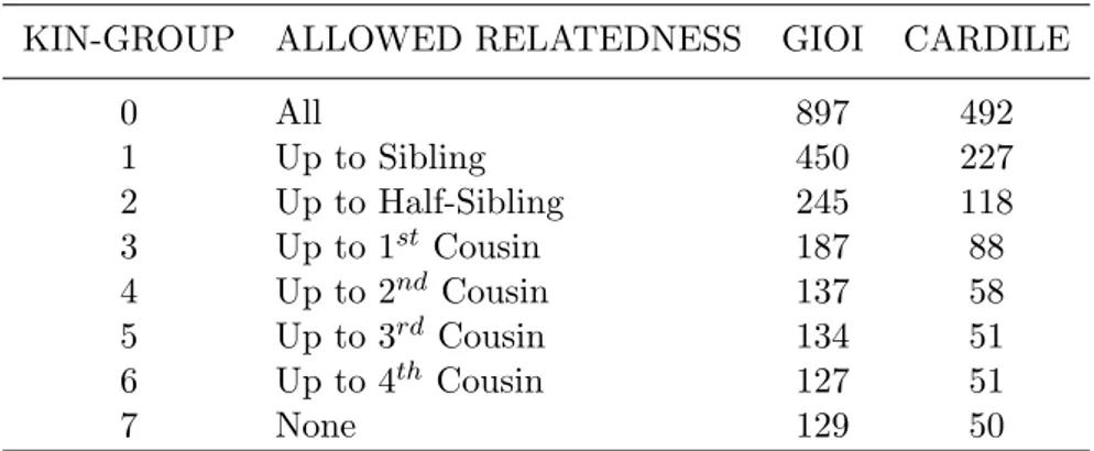
Using inferred genealogical relationships, we created 8 kin-groups of samples de-fined by restricted relatedness (Table 2). Kin-group zero is the most inclusive, including all pairs of individuals, while kin-group 7 is the most exclusive, including only unrelated, or apparently unrelated, individuals. That is, estimated kinship between all pairs of individuals in this kin-group are zero. For all other kin-groups, we restrict access to the group according to relatedness thresholds as defined in Table 2. Here, we analyzed all pairs of individuals and removed one element of the pair when their kinship is greater than the degree of allowed relatedness.

3.3.3 Marker Numbers

Our approach for studying the effect of numbers of markers on the performance of structure was to create a set of natural experiments by analyzing pairs of

pop-Table 2: Features and number of individuals for kin-groups

KIN-GROUP ALLOWED RELATEDNESS GIOI CARDILE

0 All 897 492 1 Up to Sibling 450 227 2 Up to Half-Sibling 245 118 3 Up to 1st Cousin 187 88 4 Up to 2nd Cousin 137 58 5 Up to 3rd _{Cousin 134 51} 6 Up to 4th Cousin 127 51 7 None 129 50

ulations from publicly-available data sets of human populations. For the initial analysis, we considered the dataset of Wang et al. [5], which is comprised of the original CEPH HGDP populations with an additional 24 Native American popu-lations, herein referred to as the ‘STR678’ dataset. In total, this dataset contains 78 populations, giving us a possible 3003 population pairs, typed at 678 autosomal microsatellites. For comparison to another commonly used genetic marker system, we used the dataset of Conrad et al. [116], herein referred to as the ‘SNP’ dataset. This dataset contains 53 (reported as 52, but Han is divided into “Han” and “Han-NChina”) populations typed at 2834 single-nucleotide polymorphisms, giving us 1378 possible population pairs. For the testing of informativeness of markers, we considered the original 377 autosomal microsatellite dataset of Rosenberg et al. [2], herein referred to as the ‘CEPH377’ dataset. This dataset was used because it is the dataset in which Rosenberg [66] identified informativeness of markers. Here we have 52 populations, giving us 1326 possible population pairs. Datasets are summarized in Table 3.

Table 3: Datasets included in this study, showing number of populations (Npops),

number of markers (Nmarkers), marker types (MarkerType), and number of possible population pairs considered (PopPairs)

Dataset Npops Nmarkers MarkerType PopPairs Citation

Wang 78 678 Microsat 3003 Wang et al. (2007) CEPH377 52 377 Microsat 1326 Rosenberg et al. (2003)

SNP 43 2834 SNP 1378 Conrad et al. (2006)