DOTTORATO DI RICERCA IN FISICA
ROBERTO CATALANO
EXPERIMENTAL AND MODELING METHODS
TO STUDY RADON TRANSPORT PROCESSES IN
POROUS MEDIA
P
H.D. T
HESISPh.D. Coordinator: Chiar.mo Prof. F. RIGGI Tutor: Chiar.ma Prof.ssa G. IMMÉ
I
Introduction ………...
1Chapter 1
Radon diffusion models ……….
41.1 Characteristics of radon and its decay products ………...……….. 4
1.2 Radon exhalation ……… 6
1.3 Theory of radon diffusion ………... 12
1.3.1 Plate sheet model ………. 12
1.3.2 Infinite source model ………... 18
1.3.3 Radon transport in dry, cracked soil ……… 20
1.3.4 Radon transport in unsaturated soil ………. 24
Chapter 2
Radon transport in porous materials: RnMod3d model ………...
322.1 Basic definitions ………. 32
2.2 Radon transport equation ……… 34
2.3 Soil-gas transport equation ………. 38
2.4 RnMod3d treatment of radon and soil gas ……….. 41
2.5 Finite-volume method ………. 43 2.5.1 Solution procedure ………... 45 2.5.2 Boundary conditions ……… 48 2.5.3 A study case ………... 49 2.5.4 Special considerations ………. 51 2.5.5 Model limitations ………. 52
II 3.1 Tectonic structure ………... 53 3.1.1 Eastern Sicily ………... 57 3.2 Mt. Etna ……….. 58 3.2.1 Site location ………. 62 3.3 Experimental devices ……….. 64
3.3.1 Genitron AlphaGUARD ionization chamber ……….. 65
3.3.2 Durridge RAD7 solid state detector ……… 67
3.3.3 CR-39 nuclear track solid state detector ……….. 69
3.4 Radon transport in fracturated porous media ……….. 70
3.4.1 Results and discussion ………. 71
3.5 In-soil radon vertical profile ………... 75
3.5.1 Results and discussion ………. 76
Chapter 4
Experimental set-up and procedure ……….
804.1 Laboratory facility ……….. 81
4.1.1 Radon concentration determination ………. 85
4.1.2 Temperature variations ……… 85
4.2 Radon source characterization ……… 87
4.2.1 Thoron attenuation inside the vessel………. 91
4.3 Radon detectors intercalibration ………. 93
4.4 Material properties ……….. 100
4.4.1 Grain size, density and porosity ………... 100
4.4.2 Radium content ……… 103
4.4.3 Radon emanation coefficient ………... 103
III
5.1 Sample characteristics ……… 106
5.2 Experimental procedures and analysis methods ………. 109
5.3 Experiments with upward advective transport ………... 112
5.3.1 Model description ……… 113
5.3.2 Results and discussion ………. 116
5.4 Experiments with temperature variations ………... 124
5.4.1 Results and discussion ………. 126
5.5 Considerations on samples porosity ………... 134
Concluding remarks and future perspectives ………...
137Appendix A ……….………...
140Introduction
Radon is a naturally occurring radioactive gas that is produced in the Earth’s crust as a result of alpha-decay of radium and is free to migrate through soil, either by molecular diffusion or by advection, and be released to the atmosphere where his behavior and distribution are mainly governed by meteorological processes. Advec-tion, in particular, may transfer radon over a wide range of distances, depending on the porosity and on the velocity of the carrier fluid. Due to its unique properties, soil gas radon has been established as a powerful tracer used for a variety of purposes, such as exploring uranium ores, locating geothermal resources and hydrocarbon deposits, mapping geological faults, predicting seismic activity or volcanic eruptions and testing atmospheric transport models. Much attention has also been paid to the health radiological hazard due to increased radon concentrations in the living and working environment.
In order to exploit radon profiles for geophysical purposes and also to predict its entry indoors, it is necessary to study its transport through porous soils. The complexity ge-nerated by the presence of a great number of uncontrollable and varying parameters and processes affecting the generation of radon in the soil grains and its transport in the source medium (pore-water distribution, permeability, porosity, radium content, radon emanation coefficient, advection, …), has led to many theoretical and/or laboratory studies. To measure these quantities in situ, in fact, it is not only hard, it is almost impossible to keep them constant during an experiment. Moreover, soil, as it is found
in situ, is inhomogeneous due to mixing of different layers by geological and/or
human activity, and it is influenced by flora and fauna presence, etc. The complexity is even larger if one considers, for example, that radon diffusion is mainly governed by porosity but not strongly influenced by pore size or pore size distribution.
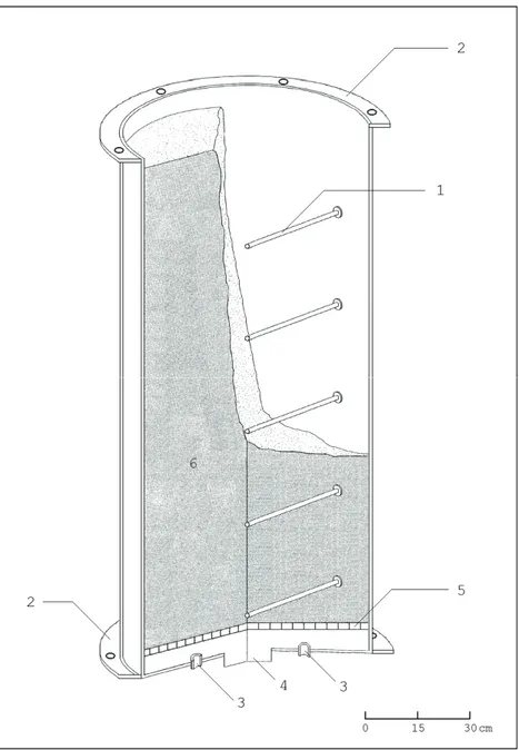
For these reasons, laboratory measurements are preferred, allowing for experiments to be conducted under well-specified and controlled conditions. This approach constitu-tes the main basis for the study presented in this thesis. Therefore, a laboratory facility was built consisting of a large cylindrical vessel, homogeneously filled with different materials, with inserted sleeves that allow measurements of radon concentra-tions in the sample gas at various depths under the sample column surface. The vessel can be closed with a stainless steel cover, the space under the cover above the sample simulating a crawl space, and, in addition, a nearly homogeneous air-flow pattern can be induced in the column by means of two inlets at the bottom of the vessel. The results of the laboratory measurements are compared with expected concentrations, according to a transport model developed by C.E. Andersen (Risø National Laborato-ry, Denmark) and suitably adapted for our purposes.
The main goal of the present study is to better understand how some parameters could affect radon transport in porous media, through both in situ and laboratory measure-ments. In chapter 1 a brief introduction to the radon characteristics is given together with the description of some of the most widely-used and reliable models to describe the radon transport in porous media. In chapter 2, the physics of radon transport in porous materials is outlined in the framework of RnMod3d derived by Andersen. The derivation is made such that the mathematical equations remain applicable for multi-phase transport in inhomogeneous media, i.e. for a porous medium containing a solid, liquid and gas phase. In this respect, the description is ‘broader’ than necessary to ac-count for the transport phenomena studied with the radon vessel.
Chapters 3, 4 and 5 cover the experimental methods and techniques. In particular, in chapter 3, in situ measurements of radon activity concentration, together with soil tho-ron and carbon dioxide efflux on Mt. Etna volcano are discussed. Both horizontal and vertical profiles of radon activity concentration were studied, even in the close proxi-mity of active faults. A comparison between experimental data and model calcula-tions has been also performed. In chapter 4, the laboratory facility installed at the Environmental Physics Laboratory of the Department of Physics and Astronomy (Uni-versity of Catania) is described in detail, with a description of the procedures and
equipment for measuring the material sample pore-air radon concentration The properties of the different sample materials (volcanic sand, volcanic rock, marble sand and clay), important for radon generation and radon transport are described in this chapter as well. Finally, in chapter 5, the results of measurements with steady-state combined diffusive and advective transport in low-moisture samples for different air-flow rates, temperatures and porosity are discussed and compared with analytical solutions of the governing differential equations given by 3D radon transport model. Finally, concluding remarks are drawn on the experimental extracted in particular in laboratory measurements at controlled conditions and on the comparison of the data with radon transport model.
Future perspectives of this kind of study are envisaged because it represents a notice-able tool from different points of view, in particular i) for radioprotection by establi-shing optimal conditions of the materials, in particular building materials to mitigate indoor radon risk, ii) for geophysical investigation to enlighten on the role of radon gas as precursor of geodynamical events, in particular magma up-rise, but more stu-dies in this direction are yet necessary.
Chapter 1
Radon diffusion models
1.1 Characteristics of radon and its decay products
Radon is a naturally occurring radioactive gas and it is one of the products of the natural decay chains of uranium and thorium, which are present in soil and rocks with varying concentrations according to the specific mineralogical and geological cha-racteristics. It exists in three different isotopes: 222Rn, member of 238U series, with an half life of 3.82 days, 220Rn (also called thoron), member of 232Th series, with an half life of 54.5 s and 219Rn, member of 235U series, with an half life of only 3.92 s. In figure 1.1 are shown the radioactive decay chains.
Owing to its higher half life, the most important of them is 222Rn, the daughter of
226
Ra. Afterits production in soil or rock, 222Rn can leave the terrestrial crust either by molecular diffusion or by convection and enter the atmosphere where its behavior and distribution are mainly governed by meteorological processes. The radon decay products are radioactive isotopes of Po, Bi, Pb and Tl and they easily attach to aerosol particles present in air. In table 1.1 the principal decay characteristics of 222Rn and
220
Rn are shown, including properties of their respective parent radionuclides and their short-lived decay products.
Table 1.1 - Principal decay characteristics of 222Rn and 220Rn
Radionuclide Half life Radiation E (MeV) E! (MeV)
226Ra 1600 y 4.78 (94.3%) 0.186 (3.3%) 4.69 (5.7%) 222Rn 3.824 d 5.49 (100%) - 218Po 3.05 m 6.00 (100%) - 214Pb 26.8 m ",! - 0.295 (19%) 0.352 (36%) 214Bi 19.7 m " - 0.609 (47%) 1.120 (15%) 1.760 (16%) 214Po 164 µs 7.69 (100%) - ---224Ra 3.66 d 5.45 (6%) 0.241 (3.9%) 5.68 (94%) 220 Rn 55.6 s 6.29 (100%) - 216 Po 0.15 s 6.78 (100%) - 212 Pb 10.64 h ",! - 0.239 (47%) 0.300 (3.2%) 212 Bi 1.01 h ,",! 6.05 (25%) 0.727 (11.8%) 6.09 (10%) 1.620 (2.8%) 212Po 298 ns 8.78 (100%) - 208Tl 3.05 m #,! - 0.511 (23%) 0.583 (86%) 0.860 (12%) 2.614 (100%)
The production of 222Rn depends on the activity concentrations of 226Ra in the earth’s crust. Trace concentrations of radium of various levels are present in soil,
rock, water and building materials. Some estimates of the activity concentration of the uranium and thorium series in soil are reported in table 1.2.
Table 1.2 - Activity concentration in some rocks
Type of rock Example
Concentration (Bq kg-1)
---
226Ra 228Ra
---
Average Range Average Range
Acid intrusive Granite 78 1 – 370 111 0.4 – 1030
Basic extrusive Basalt 11 0.4 – 41 10 0.2 – 36
Chemical sedimentary Limestone 45 0.4 – 340 60 0.1 – 540
Detrital sedimentary Clay, shale, sandstone
60 1 – 990 50 0.8 – 1470
Metamorphosed igneous Gneiss 50 1 – 1800 60 0.4 – 420
Metamorphosed sedi-mentary
Schist 37 1 - 660 49 0.4 - 370
1.2 Radon exhalation
Radon enters the atmosphere mainly by crossing the soil-air interface. The contri-butions of other sources such as oceans, lakes and rivers are relatively small. Radon from ground water or natural gas released into enclosed spaces may sometimes be important.
Since soil has 103-104 times higher gas concentrations than the normal surround-ding atmosphere, there is a great radon concentration gradient between such materials and open air. This gradient is permanently maintained by the constant generation of radon by its long-lived parent predecessor from the 238U series present in the material. The amount of radon activity released from the surface expressed in Bq m-2 s-1 is called the exhalation rate. Mechanisms governing the exhalation of radon from the soil are illustrated in figure 1.2. The exhalation rate depends on the emanation and transport of radon in the material.
Figure 1.2 - Radon emanation from soil and building material
When radium decays in a mineral substance, the resulting radon atoms must first emanate from the grains into the air-filled pore space. The fraction of radon formed that enters the pores is commonly known as the emanation fraction, emanation power or emanation coefficient. The emanation fraction consists of two components: recoil and diffusion. Since the diffusion coefficient of gases in solid grain materials is very low, it is assumed that the main portion of the emanation fraction comes from the recoil process. Following the alpha decay of radium, radon atoms possess sufficient kinetic energy to move from the site of generation. The kinetic energy of the 222Rn is about 86 keV. The range of 222Rn is between 20 and 710 nm for common materials, 100 nm for water and 63 µm for air. The radon atom could be ejected from the grain as a result of the recoil, provided it was close to the surface, and was kicked in an outward direction. In the same way, the radon atom could be ejected to a micro-fissure in the mineral grain. Further transport in the micro-micro-fissure is by diffusion. The recoil process inside the grain is shown in figure 1.3.
Figure 1.3 - Principles of radon emanation from a mineral grain. Case (1). When radium decays, a radium atom and an alpha particle are formed. The radon atom is moved into an adjacent crystal by a recoil effect from the ejected alpha particle. Case (2). The radon atom is moved through the crystal. Case (3). The radon atom is moved from the crystal to a micro-fissure or the air in an adjacent pore. It is assumed that further transport is by diffusion.
Although the emanation fraction can theoretically be assessed under some well-defined conditions, the results are generally much lower than the values of this parameter obtained experimentally. It is assumed that the large discrepancy between measured and calculated fractions is partly due to uneven distribution of radium, which could occupy places on or near the surface of the grains, and also partially due to radiation damage of the crystalline structure in the vicinity of the newly created radon atom.
The emanation fraction can be strongly affected by water content in the material. This impact of moisture is illustrated in figure 1.4 where relative changes of the ema-nation fraction are shown as a function of the water content in samples of uranium tailings.
Figure 1.4 - The effect of water content on the 222Rn emanation fraction
The emanation increases with increasing-soil moisture content, first quickly and later more slowly, in a way that can be considered almost constant in the normal range of soil moisture content (between 2% and saturation).
This increasing in the emanation fraction can be explained by the lower recoil range of radon atoms in water than in the air. If the pore space contains water, the ejected recoil most often will be brought to rest in liquid as sketched in the upper part of figure 1.5 and the radon atom is then free to diffuse from the water or be transported by it [Kigoshi, 1971]. If the interstitial space is dry (i.e. filled only with soil gas) and not wide enough to stop the recoiling radon, it enters a neighboring grain, apparently immobilizing itself as shown in the lower part of figure 1.5. It is, however, less isolated than if it failed to exit its grain of origin, the reason being that radiation damage extends to it from where it entered its new grain. This damage turns out to be etchable by exposure to water [Fleischer, 1980]. Hence, if the originally dry grains become wet before the radon has decayed, it can be released into the interstitial space.
Figure 1.5 - Models of two radon-release mechanism: (top) the recoiling
222Rn nucleus is stopped by water in the intergranular material; (bottom)
the nucleus recoils into an adjacent grain and damage track is later removed chemically by the intergranular liquid, releasing the recoil nucleus.
In addition to the moisture effect, dependence of the emanation fraction on grain size and temperature has also been observed [Markkanen and Arvela, 1992]. Small grain size soils, such as clay, display maximum emanation at about 10%-15% water content. The ratio of the maximum emanation fraction to that of a dry sample also decreases as the grain size increases. A rise in temperature also causes an increase in the emanation fraction, which is probably due to the reduced adsorption of radon. Different types of soil show different emanation fractions, which are generally about five times higher for 222Rn (in the range 0.01 - 0.5) than 220Rn (in the range 2 · 10-4 - 6·10-2). Measurements of the emanation fractions of various building materials revealed a slightly lower values than in soils, namely in the range of 2·10-4 - 3·10-2 for 222Rn and from 2·10-4 - 5·10-2 for 220Rn [Sabol and Weng, 1995].
Some emanated radon atoms, after their penetration through the material pores, may finally reach the surface before decaying. Radon gas and its movement in mate-rial follows some well-known physical laws. There are essentially two mechanisms of radon transport in material: molecular diffusion and forced advection.
In diffusive transport, radon flows in a direction opposite to that of the increasing concentration gradient. Fick’s law describes the process. It is possible to derive the expression for the radon fluence rate in Bq m-2 s-1 for specified geometric conditions. Assuming the ground to be a porous mass of homogeneous material semi-infinite in extent, the radon fluence JD emerging at the surface can be given as [UNSCEAR,
1988]: 5 . 0 ! " # $ % &
'
(
)
(
Rn e Rn Ra D D f C J (1.1)where CRa is the activity concentration of 226Ra in soil material (Bq kg-1), Rn is the
decay constant of 222Rn (2.1 á 106 s-1), f is the emanation fraction, ! is the density (kg
m-3), De is the effective diffusion coefficient (m2 s-1) and " is the porosity, all of these
parameters referred to soil material.
A similar expression can be written for a building element, such as a wall or
floor,considering it as a semi-infinite slabof porous material[SabolandWeng, 1995]:
5 . 0 -5 . 0 tanh ! " # $ % ! " # $ % & ' ( ' ( ) ( Rn e Rn e Rn Ra D D d D f C J (1.2)
where d is the thickness (m) of the slab and the other symbols have the same meaning as in equation (1.1), but in this case the parameters refer to the building material. The expressions(1.1) and (1.2) are the same apart from the hyperbolic term in the second equation. This term takes into account the finite thickness of the considered slab and is always less than unity.
Since the main mechanism governing the entry of radon into the atmosphere from the surface of the earth is the diffusion, the radon fluence rate can be calculated by using appropriate parameters in equation (1.1). Representative values of these
parameters and CRa = 40 Bq m-3 yield JD = 0.026 Bq m-2 s-1 which is quite close to the
The other mechanism affecting the movement of radon from the earth into a building is forced advection. In this case the movement of radon is caused by the slightly negative pressure differences (underpressure) that usually exist between the indoor and outdoor atmospheres. Underpressure inside a building can be created by two mechanisms: wind blowing on the building and heating inside the building. Some other factors such as changes in barometric pressure and negative pressure generated by mechanical ventilation, may sometimes also be important.
1.3 Theory of radon diffusion
Different models have been proposed to describe radon diffusion. In this section we will give a brief review of some of them.
1.3.1 Plate sheet model
One of the most reliable models to describe radon diffusion is the plane sheet model. The molecular diffusion is considered in one direction only and, for any stable element, can be described by Fick’s second law [Gauthier et al., 1999]:
2 2 z C D t C * * & * * (1.3)
where C is the concentration of the element and D the diffusion coefficient along the
z-direction. This equation admits a solution C(z, t) which is constrained by the initial
and boundary conditions ( C = C0 at t = 0 and ,a+z+a; C = 0 at t -0and z = +a):
. /
!
!
"
# $ %& % ' ( %) % * + , , -. / / 0 13 2 4 , -. / 0 1 2 4 , , -. / / 0 1 2 3 $ 0 n 2 2 2 0 4 1 2 2 1 2 cos 1 2 1 4 ) , ( a t n D a z n n C t z C n5
5
5
(1.4)where a is the half-width of the slab.
In order to take into account that radon is a radioactive gas, equation (1.3) has to
be modified for radon by adding a production term from its parent 226Ra and a decay
term, which leads to:
6 7
6 7
6 7
6 7
2 2 Rn z D Rn Ra t Rn Rn Ra 8 8 2 3 $ 8 89
9
(1.5)where brackets represent concentrations (in atoms á g-1), Ra and Rn are the decay
constants of 226Ra and 222Rn, respectively. Defining the function K(z, t) as:
6 7
( , )6 7
exp( ) ) , (z t Rn z t Ra t K Rn Rn Ra 9 9 9 , , -. / / 0 1 ,, -. // 0 1 3 $ (1.6)and introducing K(z, t) in equation (1.5), it yields:
2 2 z K D t K 8 8 $ 8 8 (1.7)
which is the Fick’s second law expressed for the function K(z, t). Nevertheless the solution of equation (1.7) cannot be merely obtained by combining the solution of the general Fick’s second law (1.3) with the substitution (1.6) because the two functions
K(z, t) and [Rn] (z, t) do not admit the same initial and boundary conditions. These
conditions, for [Rn] (z, t), are:
6 7
!
z6 7
Rn6 7
Ra Rn Ra eq 0 , Rn $ $ $ 9 9 for 3a:z:a, t$06 7
Rn!
z,t $0 for z$3a, z$a(the atmosphere is considered as a reservoir of concentration C = 0) that means for
K
!
z,0 $0 for 3a:z:a, t$0K
!
z,t $36 7
Rneq exp 9Rn t!
for z$3a, z$aFick’s law is usually solved for plane sheet geometry by separation of variables but this method is unsuccessful for such initial and boundary conditions. Several studies have been done for heat conduction in a slab having an initial zero temperature and
surfaces maintained at the temperature T(t) = Vexp(vt) [Gauthier et al., 1999],
obta-ining:
!
6 7
!
2 ,, -. // 0 1 ,, -. // 0 1 3 $ cosh cosh exp , K D a D z t Rn t z Rn Rn Rn eq 9 9 9 (1.8)6 7
!
!
!
!
!
"
# $ 2 ; < = > ? @ ,, -. // 0 1 2 2 2 ,, -. // 0 13 2 3 2 0 2 2 2 2 2 2 2 1 2 cos 1 2 4 1 1 2 4 1 2 exp 1 4 n Rn n eq a z n D n a n a Dt n Rn5
5
9
5
5
and therefore, combining with (1.6):
6 7
!
6 7 6 7
2 ,, -. // 0 1 ,, -. // 0 1 3 $ cosh cosh , D a D z Rn Rn t z Rn Rn Rn eq eq 9 9 (1.9)6 7
!
!
!
!
!
"
# $ 2 ; < = > ? @ ,, -. // 0 1 2 2 2 , , -. / / 0 1 ,, -. // 0 1 2 2 3 3 2 0 2 2 2 2 2 2 2 1 2 cos 1 2 4 1 1 2 4 1 2 exp 1 4 n Rn Rn n eq a z n D n a n t a D n Rn 5 5 9 9 5 5By multiplying by Rn both sides of the equation (1.9), we obtain the activity of
! ! ! !
2 , , -. / / 0 1 , , -. / / 0 1 3 $ cosh cosh , D a D z Ra Ra t z Rn Rn Rn 9 9 (1.10)!
!
!
!
!
!
"
# $ 2 ; < = > ? @ ,, -. // 0 1 2 2 2 , , -. / / 0 1 ,, -. // 0 1 2 2 3 3 2 0 2 2 2 2 2 2 2 1 2 cos 1 2 4 1 1 2 4 1 2 exp 1 4 n Rn Rn n a z n D n a n t a D n Ra 5 5 9 9 5 5where (Rn) and (Ra) represent the activity of 226Ra and 222Rn, respectively.
Knowing this function Rn(z, t) allows calculation of the radon concentration at
each point of the slab for a given diffusion coefficient and at a given time. Figure 1.6
shows the diffusion profiles derived from the equation (1.10) for 0:z :a and
com-pared with the solution obtained for a stable element (equation (1.4); Fig. 1.6a). Figu-res 1.6a and 1.6b pFigu-resent highly similar patterns for diffusion experiments shorter
than 104 seconds, then the effect of 222Rn radioactive ingrowth becomes more and
more important, counterbalancing the effect of diffusion. In fact, a steady-state profile
is reached, for which diffusion is exactly balanced by radon production from 226Ra.
Such steady-state profiles are governed by the following equation (Gauthier et al., 1999):
!
! ! !
cosh cosh , ,, -. // 0 1 ,, -. // 0 1 3 $ # D a D z Ra Ra z Rn Rn Rn 9 9 (1.11)and strongly depend on
A
$a9
Rn/D (figure 1.6c). For low values of ! (A
:0.1),the 222Rn radioactive ingrowth is negligible and radon behaves like a stable element.
On the other hand, for high values of ! (
A
B50), diffusion processes are too slow andFigure 1.6 - Diffusion profiles in a half-slab stable element (a), and for radon
(b, c). (a) Curves are drawn from equation (1.4) with a = 10-2 m and D = 10
-10
m2 s-1. Values on the curves refer to the duration t (in seconds) of the diffusion process. When t tends towards infinity, the concentration C becomes zero in all the slab. (b) Curves are drawn from equation (1.10) with
a = 10-2 m and D = 10-10 m2 s-1. After a sufficient time the system reaches a
steady-state for which diffusion is exactly balanced by radioactive ingrowth. (c) Steady-state (t = ) diffusion profiles drawn from equation (1.11);
numbers on diffusion curves refer to values of
A
$a9
Rn/D.The inverse problem for which radon concentration is known at a given t and z can also be considered and allows determination of the diffusion coefficient D. Such
an approach can be attempted by studying the bulk variation of radon concentration, expressed as a fractional loss f defined by (Gauthier et al., 1999):
i t i N N N f $ 3 (1.12)
where Ni is the initial number of radon atoms before heating and Nt the remaining
number of radon atoms at the end of heating. Ni and Nt are obtained by integrating
over the thickness the differential concentrations "n = [Rn] (z, t) #S dz, where # is the volumic mass of the melt and S the surface area of the slab. Thus, f is given by:
6 7
!
6 7
!
6 7
Rn!
z dz dz t z Rn dz z Rn f a a a a a a 0 , , 0 ,C
C
C
3 3 3 3 $ (1.13)After integration of (1.9), we obtain:
6 7
eq a a i N a S Rn N $C
E
$2D
3 (1.14) and: $26 7
326 7
tanh 2 D a D Rn S Rn S a N Rn Rn eq eq t 9 9 D D (1.15)6 7
!
!
"
# $ 2 2 , , -. / / 0 1 ,, -. // 0 1 2 2 3 2 0 2 2 2 2 2 2 2 4 1 2 4 1 2 exp 16 n Rn Rn eq D a n t a D n Rn S a5
9
9
5
5
D
!
!
"
# $ 2 2 , , -. / / 0 1 ,, -. // 0 1 2 2 3 3 $ 0 2 2 2 2 2 2 2 4 1 2 4 1 2 exp 8 tanh n Rn Rn Rn Rn D a n t a D n D a D a f 5 9 9 5 5 9 9 (1.16)This relation allows calculation of f at a given D and t, and also estimation of D once f, obtained from gamma-ray measurements, and t are known.
As shown in Figure 1.6c, the maximum 222Rn loss obtained for infinite time of
diffusion, depends on
A
$a9
Rn/D and tends toward 1/2 tanh !/!. For values of !ranging between 0.1 and 50, f varies from 18.9% to only 1%. For a given diffusion coefficient, the maximum fractional loss is directly constrained by the thickness of the slab.
1.3.2 Infinite source model
Letusconsideranearthmodelin which a radon infinite source with concentration
C0 is overlain by an overburden of thickness h, which contains no radon sources. This
model resembles the study area where measured radon production rate of the overburden is zero. In this case the radon transportation equation in the overburden can be written as [Wattananikorn et al., 1998]:
0 2 2 $ 3 2 D dz dC D v dz C d
9
(1.17)where C is the radon concentration at any depth z, v is the gas flow velocity (positive upward), D is the diffusion coefficient of radon and is the decay constant. The solution of (1.17) is:
; ; < = > > ? @ , , -. / / 0 1 2 , -. / 0 1 ; ; < = > > ? @ , , -. / / 0 1 2 , -. / 0 1 ;< = >? @ 3 $ h D D v z D D v D z h v C C 2 sinh 2 sinh 2 ) ( exp 2 2 0
9
9
(1.18)From (1.18), if the depth of the source h and the diffusion coefficient D are known, the value of flow velocity v may be found from the radon concentration C measured at two different depths. Figure 1.7 is a graph showing the relationship bet-ween the ratio of radon concentration at 50 cm and 100 cm depths (Cz = 50 / Cz = 100)
versus an upward flow velocity v (in terms of
9
D), for the case of an earth model having h = 20 m and D = 0.036 cm2/s.Figure 1.7 - Relation between the ratio of radon concentration at 50 and 100 cm depths, versus an upward flow velocity
Figure 1.8 - Correlation between the ratio of radon concentration for flow rate velocities v and zero, versus an upward flow velocity v, in the case of 50 and 100 cm depths.
In any earthquake event the change in radon concentration in the overburden may be induced by the change in flow velocity v. However, the change in concentration C caused by flow velocity change depends on the depth of measurement. Figure 1.8
shows such correlation that is derived from (1.18) for the same earth model mentioned earlier. From the figure it is seen that the change in the value of v causes more change in radon concentration C at 50 cm than at 100 cm depth. This fact must be taken into consideration if deep hole radon measurement is used to reduce the near surface effects due to meteorological parameters.
1.3.3 Radon transport in dry, cracked soil
A model of radon transport in dry and cracked soil, proposed by Holford et al. [1993], starts from the diffusive flux density in soil (Fd), that is the mass of radon
transported per unit time in bulk cross-sectional area of soil by molecular diffusion, defined by Fick’s law for molecular diffusion:
j ij d x nC D Fi 8 8 3 $ ( ) (1.19)
where Dij is the diffusion coefficient for radon in dry soil, i and j are subscripts
indicating direction and are summed over the range i = 1, 2 and j = 1, 2, C is the concentration of radon gas in air, defined as the mass of radon per unit volume of air,
n is the total porosity of the soil (ratio of the volume of void space to the total volume
of soil), and nC is the mass of radon transported in dry soil per unit bulk volume of soil. The diffusion coefficient for radon in dry soil is defined as [Holford et al., 1993]:
ij A ij D
D $
F
(1.20)where DA is the diffusion coefficient for radon in pure air and !ij is the coefficient of
tortuosity of the soil. The diffusion of radon in pure air is calculated as a function of temperature and pressure, the tortuosity can be defined as the ratio of the straight-line distance between two points to the same points by way of the connected pores. The tortuosity is empirically determined to be between 0.01 and 0.66 for most soils.
The advective flux density (Fa), the mass of radon transported per unit time per unit bulk cross-sectional area of soil by air flow, is defined as:
C v
Fa i
i $ (1.21)
where vi is the Darcy’s velocity of soil air, which is defined as the volume of air
flowing per unit bulk cross-sectional area of soil per unit of time in the direction i = 1, 2. Conservation of mass results in the following continuity equation:
G
9
nC n x F t nC i i ( ) ) ( 3 2 8 8 $ 8 8 3 (1.22)where t is time, Fi is the total flux density, is the 222Rn decay coefficient, and the
source term,
G
, is the production rate of radon per unit volume of soil pore space.Substituting equations (1.19) and (1.21) into equation (1.22) and neglecting the effect of rock compressibility yields the governing equation for radon transport in dry soil:
G
9
2 3 , -. / 0 1 8 8 3 , , -. / / 0 1 8 8 8 8 $ 8 8 C C n v x x C D x t C i i j ij i (1.23)Cracks and holes are assumed to be perfectly dry, with a porosity of 1 and no production of radon. Therefore the radon transport in cracks can be described by:
!
C C v x x C D x t C i i j A i 9 3 8 8 3 , , -. / / 0 1 8 8 8 8 $ 8 8 (1.24)Now, if we consider the airflow, radon transport and air flow are coupled by Darcy’s law:
, , -. / / 0 1 2 8 8 3 $ j j ij i g x P k v
D
H
(1.25)where vi is the Darcy velocity, kij is the intrinsic permeability of the dry soil, µ is the
dynamic viscosity of air at a given temperature, P is the absolute pressure, " is the
density of air at a given temperature and gj is the gravitational acceleration vector.
Conservation of mass requires that the change of fluid mass stored within a unit volume of soil equal the net rate of fluid flow into that volume. The resulting continuity equation takes the form [Bear, 1979]:
i i x v t n 8 8 $ 8 8 3 (
D
) (D
) (1.26)Combining the continuity equation (1.26) and Darcy’s law (1.25) gives:
; ; < = > > ? @ , , -. / / 0 1 2 8 8 8 8 $ 8 8
D
D
H
D
) ( j j ij i g x P k x t n (1.27)For an ideal gas, the equation of state is:
RT MP
$
D
(1.28)where M is the molecular weight, R is the universal gas constant and T is the absolu-te absolu-temperature. For isothermal flow, then:
t P RT M t 8 8 $ 8 8
D
(1.29)Substituting equations (1.28) and (1.29) into (1.27) and assuming the effects of rock compressibility to be negligible gives an equation for isothermal air flow:
,, -. // 0 1 8 8 2 , , -. / / 0 1 8 8 8 8 $ 8 8 P g k x P x P k x t P n ij j i j ij i
D
H
H
(1.30)The permeability distribution is parabolic, with the maximum permeability at the center of the crack and an average vertical permeability of:
12
2 2
w
kC $ (1.31)
where w is the width of the crack. The horizontal permeability in the crack, kC1, is
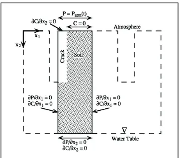
arbitrarily assigned a value several orders of magnitude larger than that of the soil. The boundary conditions at the soil surface may vary in both space and time. The boundary conditions for the flow and transport equations for the two-dimensional soil model with cracks are shown in Figure 1.9.
Figure 1.9 - Boundary conditions for a two-dimensional gas flow and radon transport simulation
At the top boundary, the atmospheric pressure is prescribed but varies with time. The concentration at the top of the soil is prescribed as zero, but the concentration at the
top of the crack is allowed to rise above zero by specifying no concentration gradient. Advective flux of radon occurs across the top cracks boundary if the velocity is not equal to zero. The left and right boundaries of the model are assumed to be axes of symmetry, at the center of the crack and at the midpoint between two cracks, respectively. The bottom boundary, at the water table, is considered to be impervious to flow and transport. The boundary conditions for the flow and transport equations for a one-dimensional soil model without cracks are exactly the same as those for the soil in the two-dimensional case.
Holford et al. [1993] have solved the governing equations for airflow and radon transport using the Galerkin finite element numerical method and a fully implicit time-weighting scheme. They compared radon transport calculations to a one-dimen-sional analytical solution of the advective-dispersion equation with radioactive decay and a linear source term. If the concentration is zero at the surface, the surface flux density is given by:
; ; < = > > ? @ ,, -. // 0 1 2 2 $ $ 2 / 1 2 2 4 2 2 ) 0 (z v v n D F
G
9
(1.32)while the concentration as a function of depth is given by:
%& % ' ( %) % * + ; ; < = > > ? @ ; ; < = > > ? @ , , -. / / 0 1 2 , -. / 0 1 2 3 $ 2 / 1 2 2 2 exp 1 2 nD D v nD v z C
G
9
(1.33)1.3.4 Radon transport in unsaturated soil
A radon transport model in unsaturated soil was proposed by Chen et al. [1995]. They started with the consideration that transient movement of soil radon to the atmosphere through the shallow subsurface can be considered as a process of volatilization and that, in general, transport of chemicals from soil into atmosphere is
complicated and difficult to predict because of the many parameters affecting sorption, motion, and persistence of gaseous and highly volatile compounds. Mechanism and factor affecting volatilization of chemicals from soil can be group into three categories: (1) those that affect the equilibrium process within the soil, (2) those that affect gas transport through the soil profile to the soil surface, and (3) those that affect the mechanism of chemical release in gas phase from the unsaturated soil to the atmosphere, as described by Spencer et al. [1990]. Volatilization can dominate the transport of highly volatile species from shallow unsaturated soil into the general environment as well as the efficiency of field application and disposal [Taylor et al., 1990]. In general, however, transport involves sorption on soil particles, movement to the soil surface and dispersal into the atmosphere.
The factors that affect gas equilibrium within soil are vapor pressures or vapor density, aqueous solubility, sorption, transformation and degradation (or decay for radon). The interaction of gas-phase chemicals with the liquid phase can be described by Henry’s constant, which governs equilibrium vapor pressure or vapor density, and Fick’s law, which describes diffusive flux rates through the media with which the gas interacts [Alzaydi et al., 1978; Thorstenson et al., 1989; Falta et al., 1989; Gierke et al., 1990].
Soil properties,suchas sizedistribution ofsoil particles and organic matter, affect transformation and degradation of chemicals [Brusseau, 1991] and emanation rates of radon [Tanner 1980, 1988; Schery et al., 1984; Nilson et al., 1991]. These factors can be described and incorporate in a general convection-diffusion equation. All of these are, however, also dependent on soil water content, characteristics of chemicals, chemical concentration and soil properties and, hence, time variations of these soil properties must also be included in the convection-diffusion equation. The sorption processes that involve radon are physical adsorption on solids and equilibrium solu-bility in liquids.
Factors that affect gas transport through the soil profile to the soil surface, in addition to those previously mentioned, are soil air permeability, which is closely
related to the soil structure and water content, and concentration and distribution of the chemical in the soil column.
The factors that affect mechanism of chemical release in gas phase from the unsaturated soil to the atmosphere are controlled by soil water content, barometric pressure and soil temperature [Tanner, 1980, 1988; Schery et al., 1984; Nilson et al., 1991; Thomas et al., 1992]. Many investigations have been done using radon and other gasses as tracers in the natural environment, and their results have shown that soil pores are the pathway of gas-phase transport but soil water content controls pore space: when soil water content increases, gas transport decreases. This is, however, a nonlinear response because saturation and drainage of soil pores and accumulation and ventilation of radon from the soil pores are not time-reversible processes [Tanner, 1980, 1988; Schery et al., 1984; Goh et al., 1991; Thomas et al., 1992]. Because the soil gas phase is highly mobile, atmospheric factors such as barometric pressure changes can have a strong impact on gas-phase transport in the field. Relatively small changes of barometric pressure can result in advective gas fluxes which are much larger than diffusive gas fluxes [Thorstenson et al., 1989; Massman, 1989]. Barome-tric pressure changes usually have an inverse influence on the movement of soil gases to the atmosphere: when barometric pressure decreases, gas flux from soil to the atmosphereincreasesbecause of the air-pumping process; increasing pressures tend to force atmospheric air into the soil and, to some extent, counteract the diffusion gradient [Tanner, 1980, 1988; Schery et al., 1984; Goh et al., 1991; Washington et al., 1992]. Because soil has a low thermal conductivity, it strongly attenuates short-period variations of air temperature with increasing depth; hence thermally dependent volatilization responds most strongly to large variations of air temperature or to seasonal changes [Goh et al., 1991; Washington et al., 1992]. The influence of wind speed on transport through unsaturated soil is still not well understood.
Starting from these considerations, Chen et al. [1995] have proposed a model to simulate transport of radon through unsaturated soil considering environmental parameters such as air temperature changes and air flow driven by barometric pressure changes. They started from a convection-diffusion equation:
I 2 8 8 3 $ 8 8 z J t CT T (1.34)
where t is the time (in days), z is the depth (in meters),I represents unspecified source or sinks of solute such as emanation and decay of soil radon and CT is the total
solute concentration in all phases (liquid, gas, sorbed). CT is defined as:
CT $
D
BCS 2J
CL2nCG (1.35) L H L L D BK C C nK C * 2 2 $D
J
!
* H D B L K nK C 2 2 $D
J
where CL is the concentration in solution (in g m-3), CS is the concentration of
chemical in the sorbed phase (in mg kg-1 of dry sand) (CS = KD × CL), CG is the
concentration in gas phase (in grams per cubic meter) (CG = K*H × CL), "B is the soil
bulk density (in kg m-3), KD is a partition or distribution coefficient (in m3 kg-1), J is
the volumetric water content (dimensionless), n is the air-filled porosity, K*H is a
modified Henry’s law constant, defined as the saturated vapor density (C*G) of the
compound divided by the aqueous solubility (C*L), both in units of mass per volume.
In addition, KD = KOC × fOC, where KOC is an organic carbon partition coefficient (in
m3 kg-1) and fOC is the organic carbon fraction of soil (dimension-less). JT is the total
solute flux density (in mg m-2 d-1) and can be expressed as (for soil radon, the unit of flux density will be Bq m-2 s-1):
AG DG CL DL T J J J J J $ 2 2 2 (1.36)
where JDL is the diffusion flux density in the liquid phase (in mg m-2 d-1), JCL is the
convection flux density in the gas phase (in mg m-2 d-1), JDG is the diffusion flux
density in the gas phase (in mg m-2 d-1) and JAG is the advection flux density in the
the advection component of transport is approximated by adding an enhancement factor in the diffusion flux of the gas phase. The total solute flux is represented by:
JS $JDL 2JCL 2JDG (1.37) L L qC dz dC q D( , ) 2 3 $
J
J
where D(J, q) is the apparent diffusion coefficient (in mm2 d-1) that includes a description of the effects upon solute movement of mechanical dispersion and both aqueous and gas phase chemical diffusion and is defined as:
J
J
J
J
, ) ( ) ( ) * ( H OG M P D q D K D q D $ 2 2 (1.38)where q is the water flux density (in m d-1), DP(J) is the efficiency diffusion
coeffi-cient in liquid phase (in m2 d-1) and it can be estimated by:
) (
)
(
J
DL
e KJDP $ OL (1.39)
where DOL is the diffusion coefficient in a pure liquid phase (in m2 d-1), # and $ are
empirical constants, reported to be 0.005:L:0.01and $ % 10 [Olsen et al., 1968], DM(q) is the mechanical dispersion coefficient that de-scribes mixing of liquid phase between large and small pores as a result of local variations in mean water flow velocity (in square meters per day) and can be estimated by:
J 9
)
(q q
DM $ (1.40)
where is the dispersivity with a range of about 2-80 mm. DOG(n) is the diffusion
coefficient for the vapor through the gas-filled porosity (in m2 d-1) and can be estima-ted by:
BARO OT
OG n D n D
D ( )$ ( )2 (1.41)
where DO is the diffusion coefficient in air (outside the porous media) (in m2 d-1) and DBARO (in m2 d-1) is the enhancement factor for barometric effects on gas advection as
mentioned above. T(n) is the dimensionless Millington and Quirk tortuosity factor given by [Jury et al., 1983]:
2 333 . 3 ) (n n S T $ J (1.42)
For nonvolatile and low-volatile gas advection of air flow through soil may be negligible. Radon gas is, however, treated as a highly volatile chemical. Changes of barometric pressures, causing air flow and resulting in gas advection, play an important role in chemical transport.
Commonly, gas advection JAG (in mm m-2 d-1) is equal to qa × CG, where CG is
thegasconcentration(in gm-3)andqa istheairfluxthrough soil (in m d-1). Barometric
pressure change is the driving force to cause air flow in soil. Adopting the derivation of the Richards equation for the water flow [Massmann, 1989], the air flow can be described by: ,, -. // 0 1 8 8 8 8 $ 8 8 3 $ 8 8 z P g K z z q t n a) ( a a) a T (
D
D
(1.43)where "a is the air density (in kg m-3), Ka is the soil air conductivity (in m d-1), PT = P
+ #agz is the total air pressure, P is the barometric (atmosphere) pressure (102 Pa), z
here is the depth (in m) and g is the gravitational acceleration. The air filled porosity,
J
J
3 $ Sn , here is a constant and can be obtained from the calculation of water con-tent, J, by the Richards equation. For an ideal gas we have a relationship:
RT MP
a $
where M is the molecular weight, R is the gas constant and T is the temperature (in kelvins). In addition, the model applies the Campbell [1974] formula to describe the relationship between the soil hydraulic conductivity Kw (in m d-1) and water content
J as: 3 2 2 ,, -. // 0 1 $ b s ws w K K
J
J
(1.45)where Kws is the saturated hydraulic conductivity and b is a constant. Kws also can be
approximated by the intrinsic permeability k (in cm2),
w w ws k g K
H
D
$ (1.46)where µw is the water dynamic viscosity (in g s-1 cm-1), and "w is the water density (in
kg m-3). Because the intrinsic permeability is independent from fluid properties, the dry-soil air conductivity Kad can be expressed from (1.46):
a a ad g k K
H
D
$ (1.47) a a w ws v KH
D
$where µa is the air dynamic viscosity (in g s-1 cm-1), and vw $
H
w/D
w is the kinematicviscosity (in cm2 s-1). Assuming that the relationship between the air-filled porosity n and the soil air conductivity Ka is:
3 2 1 2 ,, -. // 0 1 $ b s ad a n K K
J
(1.48); ; ; < = > > > ? @ 8 8 ,, -. // 0 1 8 8 $ 8 8 2 z P P n v K z t P n b s a w ws g 3 2 1
J
H
(1.49)which can be solved numerically. Surface and bottom boundary conditions are based on simulation conditions and site characteristics.
The advective gas flux density is:
L H a G a C q K C q $ * (1.50)
which is expressed in terms of concentration in the liquid phase, is added to (1.37) with the resulting solute flux equation:
L H a L w L s q C q K C dz dC q D J $3
J
(J
, ) 2 2 * (1.51)and a new numerical calculation. Because (1.49) for air flow is a nonlinear differential equation and is not very stable for numerical convergence, a numeric smoothing technique and small time steps are used to reach convergence and mass balance. This approach is especially important when the concentration of the volatile species is low and the barometric pressure change is large. In addition, some compu-tational problems are avoided by expressing barometric pressure changes relative to a standard pressure rather than in absolute terms.
Chapter 2
Radon transport in porous materials:
RnMod3d Model
In this chapter, the radon transport in isotropic porous materials, will be discus-sed in the framework of RnMod3d model derived by Andersen [1992]. The descrip-tionismadeforathree-phasesystem, i.e. for a porous medium containing solid, liquid and gas phase. Although most experiments with the radon vessel were performed with low-moisture materials, this approach is chosen because the equations for dry porousmedia forma subset of the more complex description for a three-phase system. Similar descriptions for multi-phase radon transport have been used by Rogers and
Nielson [1991, 1993] and van der Spoel et al. [1997]. An outline of the finite-volume
approach is also given.
2.1 Basic definitions
Consider a reference element V of soil. This volume may be split into three parts: Vg for the volume of grains, Vw for the volume of water, and Va for the
volume of air: a w g V V V V " ! ! (2.1)
Hence the (total) porosity !, the water porosity !w, and the air porosity !a can be
a a w V V V
#
" ! (2.2) V Vw w#
" (2.3) V Va a#
" (2.4)We define the fraction of water saturation of the pore volume (i.e. the volumetric water content) as:
# # $ w w a w V V V V " ! " (2.5)
Hence "V = 1 means that the pores are completely filled with water, whereas "V = 0
means that the soil is dry. The total mass of the reference element is:
w g M
M
M " ! (2.6)
where Mg is the mass of grain material and Mw is the mass of water. The mass of
pore air is neglected. The density of the grain material is:
g g g V M
%
" (2.7)For different types of soils #g is in the (narrow) range from 2.65 to 2.75 · 103 kg m-3.
The density for water:
w w w V M % " (2.8)
is about 1.0 · 103 kg m-3. The wet-soil density for given porosity and water content
w V g ws V M
%
$
%
#
%
" "(1& ) ! (2.9)The dry-soil density is:
g g ds V M
%
#
%
" "(1& ) (2.10)We define the amount of water per dry mass of soil (i.e. the gravimetric water content) as: V ds w ds w w g g w w g w g V V M M
$
%
%
#
#
%
%
#
#
%
%
$
1 1& " & " " " (2.11)Hence if the porosity of the soil is ! = 0.3, then full water saturation ("V = 100%)
means that the amount of water per dry mass is normally about "g = 16%.
2.2 Radon transport equation
The total activity A of 222Rn (simply referred to as “radon” in all the following) in
the reference element V may be split into three parts:
a w g A A
A
A" ! ! (2.12)
where the indices have the same meaning as in the equation (2.1). We now define the concentration of radon in the air-filled parts of the pores as:
a a a V A c " (2.13)
and the radon concentration in the water-filled parts of the pores as: w w w V A c " (2.14)
Part of the grain activity Ag is available for transport in the pore system. This is the
radon adsorbed to soil-grain surfaces: Ag,s. The immobile part ( Ag - Ag,s) is radon
produced by the “non-emanating” part of the grain radium. In line with the frame-work presented by Rogers and Nielson [1991], we introduce the sorbed radon
concentration per kg dry mass (Bq kg-1) as:
g s g s M A c " , (2.15)
where Mg is the grain mass within V.
We assume rapid sorption kinetics [Wong et al., 1992] such that the partitioning of radon between air, water and soil grains is permanently in equilibrium at any point of the soil: a w Lc c " (2.16) a s Kc c " (2.17)
where L is the Ostwald partitioning coefficient given in table 2.1 and K is the radon surface sorption coefficient [Rogers and Nielson, 1991; Nazaroff, 1992]. The equili-brium assumption simplify the problem considerably, then we can express the total
mobileradon activityby referring totheconcentrationin just onephase.Normally, the
radon concentration in the air phase ca is selected as “reference concentration”. This
approach is also used in RnMod3d. The mobile activity in V is hence given as:
V c A A
where s d w a L
#
K%
,#
'
" ! ! (2.19)is sometimes called the partition-corrected porosity. If the medium is dry and without grain sorption, we have $ = !. The equilibrium assumption is widely used in models of pollutant transport, but is not universally correct [Thomson et al., 1997]. Support for the assumption can be found in [Nazaroff et al., 1988; Nazaroff, 1992].
If radium is present only in soil grains, we define the radon generation rate per
pore volume (Bq s-1 per m3-pore) as:
g ds E E G % # # ( # % ( 1& " " (2.20)
where % is the decay constant of radon (2.09838 · 10-6 s-1), and E is the emanation rate
of radon to the soil pores (i.e. the number of atoms that emanates into water and air
per second per kg dry mass). We can write the emanation rate as E = f ARa, where f is
the fraction of emanation and ARa is the activity concentration (Bq kg-1) of 226Ra per
dry mass.
Table 2.1 - Radon solubility L in water as function of temperature [Clever, 1979] Temperature K L - 273.15 0.5249 278.15 0.4286 283.15 0.3565 288.15 0.3016 293.15 0.2593 298.15 0.2263 303.15 0.2003 308.15 0.1797
j c G t c a a " & &*) + + (' # ' (2.21)
where j is the bulk flux density (in units of Bq s-1 per m2) at time t. With the term
‘bulk’ we means that the density is measured per total cross-sectional area
perpendi-cular to j. Hence, a flux J (Bq s-1) across some plane with geometric area A and
uni-form bulk flux density j gives J = j · aA ˆ , where aˆ is a unit vector perpendicular to
the plane.
The bulk flux density consists of two, advective and diffusive, components:
d a j
j
j " ! (2.22)
Neglecting water movement, the advective flux density is given by:
q c
ja " a (2.23)
where q is the bulk flux density of soil gas (in units of m3 s-1 per m2) discussed later.
We assume that the diffusive flux can be written as:
a d D c
j "& * (2.24)
such that the bulk diffusivity accounts for radon diffusion through air and water in the pores. D is a function of temperature and pressure [Washington et al., 1994] and may therefore change in time and space. We assume that the soil-gas flow is so low that
mechanical dispersion can be ignored (i.e. D is independent of q) [Domenico et al.,
RnMod3d solves the following equation for radon transport: j c G t c a a " & &*) + + (' # ' (2.25) where a a q D c c j" & * (2.26)
is the bulk flux density of radon (in Bq s-1 per m2), and where
ca is the radon concentration in the air-filled parts of the pores (Bq m-3)
t is the time (s) s d w a L
#
K%
,#
'
" ! ! is the partition-corrected porosity (dimensionless)! is the porosity (dimensionless)
G is the radon generation rate per pore volume (Bq s-1 per m3)
% is the decay constant for radon (2.09838 · 10-6 s-1 for 222Rn)
D is the bulk diffusivity (m2 s-1)
q is a known bulk flux density of soil gas (m3 s-1 per m2)
Box 2.1 - Radon transport equations
2.3 Soil-gas transport equation
It is assumed that the flow is of the Darcy type, that the soil has a uniform
temperature (natural convection in the soil is ignored), and that !a is constant in time.
Also, it is assumed that pressure variations are small in comparison with the absolute pressure. The equation can be derived as given next.
The equation of continuity for soil gas transport is [Bird et al., 1960]:
) ( q t a a a% % # ) * & " + + (2.27)
p k
q"& *
,
(2.28)and where #a is the density of the gas (in kg m-3). For an ideal gas under isothermal
conditions, #a is proportional to the absolute pressure P(x, y, z, t) (in Pa). Hence, we
have: ) (Pq t P a "&*) + +# (2.29)
We can split the absolute pressure into three parts:
) , , , ( ) , , , (x y z t P0 ,0 gz p x y z t P " &
%
a ! (2.30)where P0 is the mean pressure at the atmospheric surface, and where p is the
distur-bance pressure field. The “aerostatic” pressure PH at depth –z below the atmospheric
surface (located at z = 0, the z-axis pointing upwards) is:
z g P
z
PH ( )" 0 &
%
a,0 (2.31)where #a,0 is the average air density at a given temperature (~ 1.3 kg m-3). Thus PH
increases of about 13 Pa per m depth.
The left-hand side of equation (2.28) can be evaluated as follows:
t t z y x p z P t P a H a + ! + " + +# # ( ( ) ( , , ,)) (2.32) t p t z PH a a + + ! + + " ( ) # # (2.33)
We limit the treatment to the situation when !a is constant in time, and we therefore
t p t P a a + + " + +# # (2.34)
On the right-hand side of equation (2.29), we assume that the disturbance pressure is
small in comparison with PH (z) such that:
q p z P q P "( H( )! ) (2.35) -PH q (2.36)
From this, we can approximate equation (2.29) as:
) (P0 q t P a "&*) + +# (2.37) or q t P P a 0 ) * & " + + # (2.38)
In the special case of homogeneous soil, we can reduce equation (2.37) and (2.28) to:
p D t P p 2 * " + + (2.39)
which is a usual diffusion equation, where:
a p P k D # , 0 " (2.40)
is the diffusivity. We observe, that without the important simplification in equation
(2.36) we would have obtained a transport equation with the term *2p2. Instead,
on-ly *2p is part of the final equation. Hence, equation (2.35) has lead to a linearization


![Table 2.1 - Radon solubility L in water as function of temperature [Clever, 1979] Temperature K L - 273.15 0.5249 278.15 0.4286 283.15 0.3565 288.15 0.3016 293.15 0.2593 298.15 0.2263 303.15 0.2003 308.15 0.1797](https://thumb-eu.123doks.com/thumbv2/123dokorg/4484050.32432/40.892.288.538.804.1041/table-radon-solubility-water-function-temperature-clever-temperature.webp)