GPSAidedInertialNavigationSystemforMini-UAVApplication UNIVERSIT´ADIPISAFacolt´adiIngegneriaLaureaSpecialisticainIngegneriadell’Automazione

(1)

UNIVERSIT ´

A DI PISA

Facolt´a di Ingegneria

Laurea Specialistica in Ingegneria dell’Automazione

Tesi di Laurea

GPS Aided Inertial Navigation System for Mini-UAV

Application

Candidato:

Valerio Niccolai

Relatori:

Prof. Mario Innocenti

Prof. Nafiz Alemdaroglu

Prof. Lorenzo Pollini

Sessione di Laurea del 09/05/2007 Anno accademico 2006/2007

(2)

Abstract

In this thesis an approach for integration between GPS and inertial navigation systems (INS) is described.

The continuous-time navigation and error equations for an n-frame INS system are derived. Using zero order hold sampling, the two sets of equations are discretized.

An extended Kalman filter for closed loop integration between the GPS and INS is derived. The filter propagates and estimates the error states, which are fed back to the INS for correction of the internal navigation states. Simulation results of the system are presented.

A description of the hardware used for practical tests is given and results are presented for a flight test.

(3)

Sommario

In questa tesi viene descritto un approccio per l’integrazione tra GPS e Sistema di Navigazione Inerziale.

Le equazioni tempo-continuo per la navigazione e l’errore vengono derivate per lo n-frame. Atraverso l’utilizzo di un campionatore zero order hold, l’insieme delle equazioni viene discretiz-zato.

Viene derivato un Filtro di Kalman Esteso per l’integrazione closed loop tra GPS ed INS. Il fil-tro evolve e fornisce stime sugli errori nelle variabili di stato; tali errori vengono refil-troazionati sulla INS per la correzione interna degli stati di navigazione. Vengono presentati risultati di simulazioni. Viene fornita una descrizione dello hardware utilizzato per i test pratici e vengono presentati i risultati di tali test.

(4)

Acknowledgment

This Master Thesis was carried out at the Aerospace Department of the Middle East Technical University in Ankara, Turkey.

I’d like to thank my examiner Prof. Dr. Mario Innocenti for giving me the opportunity of doing this thesis.

I’d like to thank all teachers and instructors at METU, especially Prof. Dr. Nafiz Alemdaroˇglu for allowing me doing this thesis.

Furthermore, I want to thank Dr. Volkan Nalbantoˇglu for his help, support and all the discus-sions throughout this project. It was a pleasure to work with him.

Thanks also go to H¨useyin Yiˇgitler for all his support, technical and personal. I hope we’ll meet again.

Thanks to all the guys at the ”Hangar”, especially to Volkan, Sercan, Serhan and Fikkri for the enjoyable and nice time there.

A special thank goes to Prof. Dr. Lorenzo Pollini from the Electrical Systems and Automation Department, faculty of Engineering, at Pisa University for the help with the sensor data acquisition.

(5)

Notations

Matrices are denoted in bold upper case letters Vectors are denoted by bold lower case letters (·)b _{variable in the body-frame}

(·)n variable in the navigation-frame (·)e _{variable in the ECEF-frame}

(·)i variable in the inertial-frame

Rb_a directional cosine matrix to transform from a- to b-frame

ω_abc angular velocity vector of b-frame w.r.t. a-frame, expressed in c-frame Ωc

ab skew symmetric representation of ωabc

(·)T matrix transpose (·)−1 _{matrix inverse}

In identity matrix of order n

0m×n zero matrix of order m × n

xK value at instant K: x(K)

˙x first order derivative of x δx error of x ˆ· estimated value ˜· measured value (·)− _{predicted value} E{·} expectation | · | magnitude k · k norm

(6)

Parto al mattino Vento e destino Sciacallo grigio argento dai magri fianchi Sappi che sono l’uomo della Leina Rivesto l’armatura sul cuore della iena. Ora sono in povertá Ora in ricchezza Desiderio, paura, libertá Bisogno di chiarezza Nella polvere un rifugio ripara dall’offesa Un ritiro per chi teme Il nemico é la resa. (Shánfara)

(7)

List of Figures

1.1 A schematic description of the proposed system with its input and output signals. . 11

1.2 Loosely coupled position aided closed loop implementation of a GPS aided INS system. KF denotes the Kalman Filter, and H the map between navigation output and GPS data. . . 12

2.1 Inertial measurement units. . . 15

3.1 Vectors that define the position between the Earth, a satellite and a user. . . 19

3.2 Multipath propagation; the solid arrow indicates the direct path, the dashed ar-rows indicate reflected path. . . 21

3.3 Illustration of a single dierence GPS. . . 23

4.1 Relations between ECEF(e-frame)-, navigation(n-frame)- and inertial(i-frame)-frame. . . 25

4.2 Body coordinate frame. . . 26

4.3 By projection of vector p onto the bases of the two orthonormal coordinate systems the directional cosine matrix relating the two coordinate systems can be found. . . 27

4.4 Coordinate system A and B referred to in the derivation of the rotation matrix Rb a a through of plane rotations. . . 28

4.5 Plane rotations. . . 29

5.1 Gravity attraction between two masses m1and m2at the distance r from each other. 34 5.2 Functional diagram of a Strap-Down INU. . . 35

7.1 Estimated and true trajectory of a typical flying sequence. . . 52

7.2 Average errors in accelerometers bias estimates. . . 53

7.3 Average errors in gyros bias estimates. . . 53

7.4 Average errors in Euler angle estimates. . . 54

7.5 Average errors in Vnorthestimates. . . 54

7.6 Average errors in Veast estimates. . . 55

7.7 Average errors in Vdownestimates. . . 55

7.8 Average errors in latitude estimates. . . 55

7.9 Average errors in longitude estimates. . . 56

7.10 Average errors in height estimates. . . 56

8.1 Navigation block diagram . . . 58

8.2 Horizon Hobby: Horizion 9 Xtra Easy II . . . 58

(11)

8.4 Crossbow Technology: Inertial System MicroNav - Block Diagram . . . 59

9.1 GPS-receiver position estimates, Latitude-Longitude plane. . . 61

9.2 GPS-receiver position estimates, 3-D trajectory. . . 62

9.3 Latitude estimate. . . 63

9.4 Longitude estimate. . . 63

9.5 Height estimate. . . 64

9.6 Height estimate between 410s and 440s. . . 64

9.7 Roll angle estimate. . . 64

9.8 Pitch angle estimate. . . 65

9.9 Yaw angle estimate. . . 65

9.10 Trajectory estimate in the Latitude-Longitode plane between 150s and 380s. . . 66

9.11 Accelerometer bias estimates. . . 66

9.12 Gyro bias estimates. . . 66

A.1 Earth shape model geometry. . . 71

C.1 The projection of a vector yk onto the subspace L(yk) corresponds to the least square estimate of the vector ykgiven the sequence {y0, y1, y2, . . . , yk−1}. Note that the prediction error is orthogonal to the subspace. . . 79

(12)

List of Tables

3.1 Typical errors that affect the pseudo-range measurement. . . 20

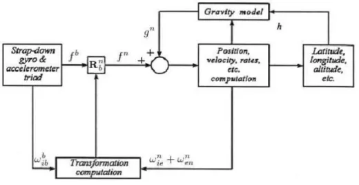
6.1 The algorithm for integration between GPS and INS data, with a ratio between the sample rates equal to r times. . . 47

8.1 Horizon Hobby: Hangar 9 Xtra Easy II specifications. . . 60

A.1 Reference ellipsoid constants. . . 75

A.2 WGS-84 ellipsoid constants. . . 75

C.1 The Kalman filter recursions in prediction form. . . 81

(13)

Chapter 1 Introduction

1.1 Background

The five basic forms of navigation are as follows, [10]:

• Pilotage, which essentially relies on recognizing landmarks to know where you are. Its older

than human kind.

• Dead Reckoning, which relies on knowing where you started from, plus some form of

heading information and some estimate of speed.

• Celestial Navigation, using time and the angles between local vertical and known celestial

objects (e.g. sun, moon or stars).

• Radio Navigation, which relies on radio-frequenciy sources with known location (including

Global Positioning System satellites).

• Inertial navigation, which relies on knowing your initial position, velocity and attitude and

thereafter measuring your attitude rates and accelerations. It is the only form of navigation that does not rely on external references.

These forms of navigation can be used in combination as well. The subject of this thesis is a combination of the fourth and fifth forms of navigation using Kalman filtering.

Kalman filtering exploits a powerful synergism between global positioning system (GPS) and

inertial navigation system (INS). This synergism is possible, in part, because the INS and GPS

have very complementary error characteristics.

Today many vehicles are equipped with global positioning system (GPS) receivers that con-stantly can provide the driver with information about the vehicles position with an accuracy in the order of 15 − 100 meters. However, the GPS receiver has two major weaknesses. The slow update rate, only once a second for most receivers, and the sensitivity to blocking of the satellite signals. This can cause problems when for example plotting a vehicles movements on a map.

Inertial navigation systems (INS) can provide position, velocity and attitude estimates at a high rate, typically 100 times per second and are, to the opposite of the GPS receiver, self contained. Instead it relies on Newtons laws of motion, from which it can be concluded that if an objects initial position, velocity and attitude are known all further positions, velocities and attitudes can be determined by integrations of the accelerations and angular rates of the object. However, due to the

(14)

integrative nature of the INS, low frequency noise and sensor biases are amplified. The unaided INS may therefore have unbounded position,velocity and attitude errors. These complementary properties make an integration of the two systems suitable.

The Kalman filter is able to take advantage on these characteristics to provide a common, in-tegrated navigation implementation with performance superior to that of either subsystem (GPS or INS). By using statistical information about the errors in both systems, it is able to combine a system with tens of meters position uncertainty (GPS) with another system whose position un-certainty degrades at kilometers per hour (INS) and achieve bounded position uncertainties in the order of centimeters [with differential GPS (DGPS)] to meters.

A key function performed by the Kalman filter is the statistical combination of GPS and INS information to track drifting parameters of the sensors in the INS. As a result, the INS can provide enhanced inertial navigation accuracy during periods when GPS signal may be lost, and improved position and velocity estimates from INS can then be used to make GPS signal reacquisition happen much faster whet the GPS signal becomes available again.

Until recently inertial measurement units (IMU) have been to expensive for private persons. But lately some low cost micro electro mechanical systems (MEMS) gyros and accelerometers have been introduced on the market. This has opened the door for development of low cost inertial navigation systems, suitable for integration with GPS-receivers.

1.2 System Overview

The purpose of the system described in this thesis is to combine GPS and INS data in an optimal way to obtain a navigation system with both higher update rate and smaller position error than the stand alone GPS-receiver. In Figure 1.1 a system overview with its different input and output signals is shown. A common integration method is to let the INS be the major navigation system and use the position estimates of the GPS-receiver to estimate and correct the errors in the INS. The integration between INS and GPS is refereed to as a GPS aided INS.

Figure 1.1: A schematic description of the proposed system with its input and output signals. Before integrating the two systems the provided data must be transformed into a common coordinate system, suitable for integration. GPS receiver provides position estimates in terms of Latitude, Longitude and Altitude. In the case of the INS it is more complicated. The accelerations and angular rates are measured with respect to the inertial frame of reference and resolved in the instrumental frame of the accelerometers and the gyros, respectively. An inertial frame is a coordinate frame in which Newtons laws of motion applies, that is in rest or in linear motion. From the instrumental frame the measurements must be transformed to the platform frame, which is the coordinate system associated with the platform onto which the accelerometers and gyros are

(15)

mounted. The platform is referred to as the inertial measurement unit (IMU). Finally the angular rates, resolved in platform coordinates are used to transform the accelerations into a common navigation frame, where they are processed and integrated with the GPS data.

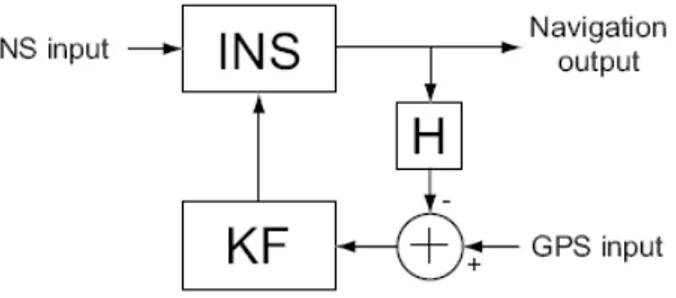
There are several approaches on how to design a GPS aided INS: tightly coupled or loosely coupled, closed or open loop, pseudo-range or position aided. In this thesis a loosely coupled position and position-velocity aided methods is proposed. Essentially this means that GPS and INS work independently and that there is no direct data exchange between them, i.e loosely coupled, and that GPS-receiver position estimates and not the estimated distances to the satellites are used (pseudo-ranges). The loosely coupled approach allows the use of a low cost of-the-shelf GPS receiver. The difference between the GPS and INS position or position and velocity estimate is used to drive an extended Kalman filter, housing a model of how the errors in the INS develops with time. The error states estimated by the filter are fed back to the INS for calibration of its internal states, resulting in a closed loop design; see Figure 1.2. A comparison between the tightly and loosely coupled approach can be found in [19].

Figure 1.2: Loosely coupled position aided closed loop implementation of a GPS aided INS system.

KF denotes the Kalman Filter, and H the map between navigation output and GPS data.

1.3 Thesis Outline

The thesis is divided into 10 chapters:

• Chapter 2 gives a short introduction to the basic principles of Inertial Navigation. The two

categories of INS are presented, namely Gimballed and Strap-down.

• Chapter 3 describes the GPS system. Error sources and possible solutions are presented. • Chapter 4 gives an introduction to the coordinate frames used throughout this thesis.

• Chapter 5 gives a short introduction to the basic physics behind inertial navigation. From this

general navigation equations are derived. Further the n-frame navigation and error dynamics are presented. Continuous time equations are discretized using a zero-order-hold model.

• Chapter 6 gives the mathematical background for the integration between the GPS and INS,

using an extended Kalman Filter.

• Chapter 7 presents simulation results of the integrated navigation system for a typical flying

(16)

• Chapter 8 gives a short description of the hardware used in the tests.

• Chapter 9 presents test results of the integrated navigation system for a real flying test. • Chapter 10 presents conclusions and further work.

(17)

Chapter 2 Inertial Navigation Systems

In this chapter, an introductory-level overview of inertial navigation systems will be given. All the fundamental terms will be defined and a basic description of the two main architecture of INS will de explained.

2.1 Fundamentals of Inertial Navigation

In order to deal with INS its necessary to define some basic concepts of inertial navigation, [10]:

• Inertia, is the property of bodies to maintain constant translational and rotational velocity,

unless disturbed by forces or torques, respectively (Newtons first law of motion).

• Inertial Reference Frame, is a coordinate frame in which Newtons laws of motion are valid.

Inertial reference frames are neither rotating nor accelerating.

• Inertial Sensors, measure rotation rate and acceleration, both of which are vector-valued

variable:

– Gyroscopes are sensors for measuring rotation: rate gyroscopes measure rotation rate, and displacement gyroscopes (also called whole-angle gyroscopes) measure rotation angle.

– Accelerometers are sensors for measuring acceleration. However, accelerometers can-not measure gravitational acceleration. That is, an accelerometer in free fall (or in orbit) has no detectable input.

The input axis of an inertial sensor defines which vector component is measured. Multi-axis sensors measure more than one component. Inertial navigation uses gyroscopes and accelerometers to maintain an estimate of the position, velocity, attitude and attitude rates of the vehicle in or on which the INS is carried, which could be a spacecraft, missile, aircraft, surface ship, submarine or land vehicle.

• Inertial Navigation System (INS), consists of the following:

– Inertial measurement unit (IMU), containing a cluster of sensors: accelerometers (two or more, but usually three) and gyroscopes (two or more, but usually three). These sen-sors are rigidly mounted to a common base to maintain the same relative orientations.

(18)

– Navigation computer, to calculate the gravitational acceleration (not measured by ac-celerometers), doubly integrate the net acceleration to maintain an estimate of the po-sition of the host vehicle and integrate the rotation rate to maintain an estimate of the attitude of the host vehicle.

There are many different designs of inertial navigation systems with different performance char-acteristics, but they fall generally into two categories:

• Gimballed • Strap-down

These are illustrated in Figure 2.1 and described in the following sections.

Figure 2.1: Inertial measurement units.

2.2 Gimballed System

2.2.1 Gimbals

A gimbal is a rigid frame with rotation bearings for isolating the inside of the frame from external rotations about the bearing axes. If the bearings could be made perfectly frictionless and the frame could be made perfectly balanced (to eliminate unbalanced torques due to acceleration), then the rotational inertia of the frame would be sufficient to isolate it from rotations of the supporting body. This level of perfection is generally not achieved in practice, however.

Alternatively, a gyroscope can be mounted inside the gimbal frame and used to detect any rota-tion of the frame due to torques from bearing fricrota-tion or frame unbalance. The detected rotarota-tional disturbance can then be used in a feedback loop to provide restoring torques on the gimbal bearings to null out all rotations of the frame about the respective gimbal bearings.

At least three gimbals are required to isolate a subsystem from host vehicle rotations about three axes, typically labeled roll,pitch and yaw axes.

(19)

The gimbals in an INS are mounted inside one another, as illustrated in Figure 2.1(b). We show three gimbals because that is the minimum number required. Three gimbals will suffice for host vehicles with limited ranges of rotation in pitch and roll, such as surface ships and land vehicles. A fourth gimbal is required for vehicles with full freedom of rotation about all three axes, such as high performance aircraft.

2.2.2 Stable platforms

The earliest INSs were developed in the mid-twentieth century, when flight-qualified computers were not fast enough for integrating the full (rotational and translational) equations of motion. As an alternative, gimbals and servo torques were used to null out the rotations of a stable platform or

stable element on which the inertial sensors were mounted, as illustrated in Figure 2.1(b).

The stable element of a gimballed system is also called inertial platform os stable table. It contains a sensor cluster of accelerometers and gyroscopes, similar to that of the strap-down INS illustrated in Figure 2.1(a).

2.2.3 Signal processing

The essential outputs of the gimballed IMU are the sensed accelerations and rotation rates. These are first compensated for errors detected during sensors- or system-level calibration. This includes compensation for gyro drift and rates due to acceleration.

The compensated gyro signals are used for controlling the gimbal to keep the platform in the desired orientation, independent on the rotations of the host vehicle. This “desired orientation” can be (and usually is) locally level, with two of the accelerometers axes horizontal and one ac-celerometer input axis vertical. This is not an inertial orientation, because the earth rotates and, and because the host vehicle can change its longitude and latitude.

The accelerometers outputs are also compensated for known errors, including compensation for gravitational accelerations which cannot be sensed and must be modeled. The gravity model used in this compensation depends on the vehicle position.

After compensation for sensor errors and gravity, the accelerometers outputs are integrated once and twice to obtain velocity and position, respectively. The position estimates are usually converted to longitude, latitude and altitude.

2.3 Strap-down system

2.3.1 Sensor cluster

In strap-down systems, the inertial sensor cluster is “strapped down” to the frame of the host vehicle, without intervening gimbals for rotational isolation, as illustrated in Figure 2.1(a). The system computer must integrate the full six-degree-of-freedom equations of motion.

2.3.2 Signal processing

Starting from the signal flow of a gimballed system, the major software functions performed by navigation computers for strap-down systems are:

(20)

• “Coordinate transformation” and “Acceleration coordinate transformation” which

essen-tially take the place of the gimbal servo loops. In effect, the strap-down software maintains virtual gimbals in the form of a coordinate transformation from the unconstrained, body-fixed sensor coordinates to the equivalent sensor coordinates of an inertial platform.

• Attitude rate compensation for accelerometers, which was not required for gimballed

sys-tems but may be required for some applications strap-down syssys-tems. The gyroscopes and gimbals of a gimballed IMU were used to isolate the accelerometers from body rotation rates, which can introduce errors such as centrifugal accelerations in rotating accelerometers. In the continuous of this thesis, all the developments will be addressed to Strap-down Systems.

2.3.3 Coordinate systems

In Strap-down inertial navigation systems the measured quantities is obtained in different coordi-nate frames and need to be transformed into a coordicoordi-nate frame suitable for processing.

A basic inertial navigation system involves at least four different frames. The accelerometers measures the platform accelerations with respect to the inertial frame of reference. The accelera-tions are resolved in the instrumental frame of the accelerometers and need to be transformed into platform coordinate frame by a fixed rotation matrix.

Gyros measure the platform angular rates relative to the inertial frame of reference and resolves this in the instrumental frame of the gyros, which are transformed into angular rates in the platform frame by a fixed rotation matrix.

From the gyro measurements a rotation matrix is calculated which transform the accelerations in the platform-frame into the used navigation frame, where they are processed to determine the velocity and position of the navigation system.

(21)

Chapter 3 Global Positioning System

There are currently two Global Navigation Satellite Systems (GNSS), namely the widely used Global Positioning System (GPS) from the U.S. Department of Defense, and the Russian Global Orbit Navigation Satellite System (GLONASS).

A third system named Galileo, which is launched by the European Union and the European Space Agency, will be in commercial operation phase in year 2008.

Because the GPS is well established and a broad range of receivers (also some relatively inex-pensive receivers) are available, this system was chosen for this project, [18].

3.1 GPS Signals

With the GPS, civilian users can only use the restricted Standard Positioning Service (SPS). The Precise Positioning Service (PPS) is only intended for the U.S. military and other authorized users. There are at least 24 satellites on six equally spread orbits around the Earth. The six orbital planes are inclined with a 55 angle with respect to the equator. The orbits are located about 20200 km above the Earths surface.

The GPS mainly provides a 3-dimensional position estimation and the accurate Coordinated Universal Time UTC. To estimate a 3-d position, the receiver needs to receive the signals of at least 4 satellites. The accuracy of the estimate depends on several factors that are discussed in the following section.

In order to compute the position at the receiver, the position of the satellites has to be known. These coordinates can roughly be calculated from the GPS almanacs that are transmitted by the satellites. For a more accurate satellite coordinate calculation, the ephemeris data, also transmitted in the satellite message, is used.

Each GPS satellite transmits the data simultaneously on the two frequencies L1 (1575.42MHz) and L2 (1227.60MHz). The data (50bit/s) is BPSK modulated and spread with binary codes (CDMA). The later are used to differentiate between the satellites. On L1, the signal is spread with a Precision or P-code and a Coarse/Acquisition or C/A-code. The signal on L2 is only spread with the P-code. While the C/A-code is publicly available (SPS), the P-code is further encrypted for a regulated access and is only known by authorized users (PPS). The C/A-code consists of 1023 samples, is transmitted at 1/10 of the fundamental GPS frequency and is repeated every 1 ms, whereas the P-code is transmitted at the fundamental frequency of 10.23 MHz and repeated every 267 days.

(22)

Figure 3.1: Vectors that define the position between the Earth, a satellite and a user. There are three observable quantities, namely the pseudo-range, the carrier phase, and the Doppler shift. The pseudo-range represents the time shift needed to correlate the received and demodulated signal with a receiver-replicated code. Since the receiver- and satellite-clocks are not perfectly synchronized, and also due to other error sources, the description pseudo-range rather than range is used.

Better performance for the position determination can be gained by measuring the carrier phase before the demodulation. This allows an accuracy down to a fraction of the wavelength, but there is a problem called integer ambiguity. Using the phase, only a fraction of a wavelength can be measured, but there remains an unknown number of whole wavelengths that fit between the satellite and the receiver. Due to high vehicle dynamics, satellite shading, and high ionosphere activity, a loss of phase lock can occur and results in a so-called cycle slip. A method to overcome this problem can be found in [1].

Finally, a Doppler shift can be measured due to the movements of a receiver. However, a Doppler shift only occurs if the receiver is moving towards to or away from a satellite. Also the satellites itself move, but, since their trajectory is predictable, this influence can be compensated. The measured Doppler shift is used to determine the receivers velocity.

The position of a particular satellite is known from the ephemeris data (ECEF coordinates) and is denoted as s in Figure 3.1. The distance d is estimated using the pseudo-range and phase measurements (the distance is obtained by multiplying the time delay with the speed of light). Adding this two vectors, one can find the user position as

u = s + d (3.1)

The measured pseudo-range estimated from each satellite (subscript k) can be expressed as ρk= ku − skk + c (δtsk+ δtr) + εk (3.2)

where the difference δtsk+ δtr multiplied with the speed of light is an error due to the clock drift

in the satellite and receiver. The remaining error components are collected in εk and described

in the following (see also Table 3.1). Disregarding εk , we see from Equation (3.2) that we have

three unknowns for the position in ECEF coordinates, and one unknown for the clock difference. Therefore, we need four satellites to solve for the 4 unknowns. Usually, there are more than four satellites available leading to an over-determined system that can be solved in a least squares sense, and provide a more accurate solution.

(23)

3.2 Error Sources

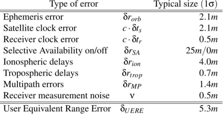
Several error sources can deteriorate the quality of the position estimation. The following para-graphs name the important sources. The size of these typical errors is collected in Table 3.1.

Type of error Typical size (1σ) Ephemeris error δrorb 2.1m

Satellite clock error c · δts 2.1m

Receiver clock error c · δtr 0.5m

Selective Availability on/off δrSA 25m/0m

Ionospheric delays δrion 4.0m

Tropospheric delays δrtrop 0.7m

Multipath errors δrMP 1.4m

Receiver measurement noise ν 0.5m User Equivalent Range Error δUERE 5.3m

Table 3.1: Typical errors that affect the pseudo-range measurement.

3.2.1 Selective availability

The U.S. Department of Defense has with Selective Availability (SA) a method, to add a clock error introduced by the satellites to affect the position determination for unauthorized users. In May 2000, this SA was removed [7] but there is no guarantee that it will not be introduced again. For civil users, this SA accounts for the largest errors. There are methods such as Differential GPS (DGPS) to reduce this error [13].

3.2.2 Atmospheric effects

Atmospheric effects introduce further errors. The troposphere is relatively close around the Earth and extends between 6 to 18 km. It is electrically neutral and non-dispersive for frequencies up to 15 GHz [24, 8]. However, the presence of water vapor, the atmospheric temperature, and the pressure cause a delay, which is the same for both frequencies L1 and L2.

The ionosphere extends roughly from 50 to 1500 km and contains a large amount of free electrons and positive ions. These cause a group delay of the signal but can also cause refraction and diffraction effects [24]. The ionospheric activity is strongly dependent on the number of sunspots. Using appropriate models and DGPS, these atmospheric effects can be significantly reduced to improve the position accuracy.

3.2.3 Orbital errors

Another error is introduced due to the inaccuracy in the ephemeris data. The Signal-in-Space User

Range Error (SIS UER) was 1.4m RMS as of April 2001 across the constellation and is expected

to decrease [5]. Replacing older Block II satellites with newer Block IIR satellites and the Legacy

Accuracy Improvement Initiative (AII) contribute to a better performance.

Data that are more accurate are available through the official Navel Surface Warfare Center together with the National Imagery and Mapping Agency, which are available a few weeks after

(24)

the observation. A large user community uses orbit products from the International GNSS Ser-vice (IGS), because they also provide predicted real-time IGS Ultra-Rapid orbit products with an accuracy of about 0.25m. More information about how IGS works can be found in [2].

3.2.4 Clock errors

The atomic clocks in the GPS satellites have to run synchronized with the GPS system time. The small difference is constantly monitored by the Master Control Station (MCS) and the errors are transmitted as coefficients of a second order polynomial [4]. The larger clock errors occur in the receiver. It varies depending on the clock quality between some µs to a few ms. Nevertheless, this clock-drift as well as the satellite clock error can be effectively removed by using DGPS [13].

3.2.5 Multipath and noise

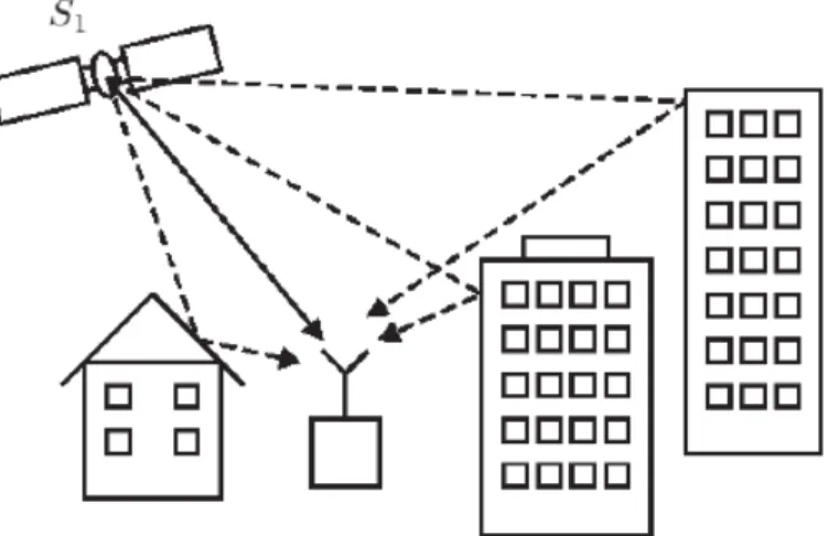
In wireless radio links, one has to deal with multipath reception. The best case is to have a direct line of sight between the transmitter and the receiver. Nonetheless, there are reflected signals that superimpose the direct signal (see Figure 3.2). These multipath reflections affect both the pseudo-range and phase measurements in a GPS receiver. Methods to decrease the effects are known from e.g. cellular radio communications [24].

Figure 3.2: Multipath propagation; the solid arrow indicates the direct path, the dashed arrows

indicate reflected path.

At last, there is also noise generated in the receiver itself and maybe in the environment. The receiver noise is depending on the antenna gain, amplifiers, receiver dynamics, and the code cor-relation methods. It can mostly be reduced by a careful and thorough hardware design.

3.3 Dilution of Precision

Another effect that affects the precision of a position estimation is caused by the satellite constella-tion. If e.g. all satellites happen to be on a straight line from the users point of view, the precision is worse than if e.g. three satellites are placed equidistant on a large circle around the user and one satellite straight above. The Dilution of Precision (DOP) [9] expresses these effects together

(25)

with the time bias errors and the other pseudo-range errors. The pseudo-range error δρ can be ob-tained from the position errors and the time error δe =£ δx δy δa c δt ¤T through a linearized equation as

δρ = H δe + δ²p (3.3)

where H is a (m × 4) matrix of partial derivatives of the Equation (3.3), with respect to the four unknown variables. δ²pis a zero mean noise term. Assuming many simplifications, one can take

the expectation of the estimated vector δ²pleading to, see [16]

E{δ ˆ² δ ˆ²T} = σ2_e(HTH)−1 (3.4) The matrix multiplication and inversion can be expressed as

(HTH)−1=     D11 D12 D13 D14 D21 D22 D23 D24 D31 D32 D33 D34 D41 D42 D43 D44     (3.5)

where each Di j ∈ ℜ represents a scale factor for the variance σ2ε. Since the diagonal elements of

that matrix relate the measurement errors with the computed position and time errors, one can find the following parameters:

HDOP =√D11+ D22 (3.6)

HDOP =pD33 (3.7)

HDOP =√D44 (3.8)

These first three DOP parameters describe the horizontal DOP, vertical DOP, and time DOP, re-spectively. Two more general DOP parameters can be calculated, namely, the position DOP and the geometric DOP

HDOP =pD11+ D22+ D33 (3.9)

HDOP =pD11+ D22+ D33+ D44 (3.10)

The total position, vertical, or time error magnitude can be estimated as the multiplication of the standard deviation σε with the desired DOP value. For example, for a GPS receiver that only

provides the PDOP, the position error magnitude is approximated as

σr= PDOP · σε (3.11)

It becomes clear that a low value indicates a good accuracy. In practice, values below 8 can be considered as fairly good. In field tests on an open area with a clear line of sight and low multipath reflections, the PDOP value usually ranged between 2 and 5.

3.4 Differential GPS

In Section 3.1, the error sources with the most influence on the position accuracy were pointed out. Except for multipath and noise errors, it is possible to reduce or even remove their effect on the position estimation. There are several combination methods available. The most common

(26)

Figure 3.3: Illustration of a single dierence GPS.

one is the single difference GPS (or differential GPS (DGPS)) as depicted in Figure 3.3. Sophis-ticated methods such as double or triple difference incorporate measured differences from several satellites.

Another technique is to use a second frequency, e.g. L2, in order to minimize the ionospheric effects. However, this method is not available to public, unauthorized users.

The single difference GPS employs one mobile receiver e.g. on a vehicle and a stationary receiver (base station). The exact coordinates of the base station are known, therefore it is possible to compute the real errors in the pseudo-range and form some correction parameters. They are transmitted to the mobile receiver over e.g. a radio link (dashed arrow in Figure 3.3). If the mobile receiver is relatively close to the base station, both received signals from the satellites experience almost the same atmospheric disturbances. The mobile receiver then uses the correction parameters to minimize or even eliminate the errors.

However, since the thermal noise in the two receivers is uncorrelated, its variance increases with the factor two. Still, it is possible to get a position accuracy of a few centimeters.

(27)

Chapter 4 Coordinate Systems

Position, velocity and attitude, referred as navigation system states, are defined with reference to coordinate frames. These frames are defined differently for the various integrated navigation system’ implementations, and there are a number of different frames in current use.

The chapter presents a survey of coordinate systems used in this thesis and transformations useful to manipulate vector variables between coordinate frames.

Last section presents the derivation of an analytical form to express the rate of change of a rotating reference frame.

4.1 Coordinate Frame Definition

This section defines the different coordinate frames and corresponding notation used in this thesis. All coordinate systems are orthogonal and right-handed Cartesian systems if not otherwise stated.

4.1.1 Inertial frame (i-frame)

An inertial frame is a coordinate frame in which Newtons laws of motions apply. Therefore the inertial frame is not accelerating or rotating, but can be in a linear motion.

The origin of the inertial coordinate system is arbitrary, and the coordinate axis may point in any three perpendicular directions. Its often preferable to let the origin of the inertial frame consist with the Earth center of mass and define his z-axis parallel to Earth’s rotation.

This frame will be referred to as the i-frame and will be denoted by the superscript i.

4.1.2 Earth-centered earth-fixed frame (ECEF, e-frame)

This coordinate system has its origin at the center of the earth and rotates with the earth.

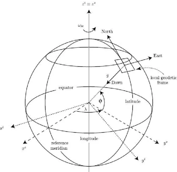
Axis definitions in current use vary. For the purpose of this thesis, the axes directions are defined as follows: the x-axis points towards the intersection between the prime meridian and the equator, the z-axis points in the direction of the mean polar axis and the y-axis completes the right hand coordinate; see Figure 4.1. The ECEF frame will be denoted by the superscript e.

As will be shown in the sequel (Section 4.2) a vector p in the i-frame is linearly related (by a rotation matrix) to a vector in the e-frame, and vice verse.

(28)

(29)

4.1.3 Navigation frame (n-frame)

This is the coordinate system often referred to in our daily life as the north, east and down direction. It will be denoted by the superscript n and also referred as Local Geodetic Frame in Figure 4.1.

Its determined by fitting at tangent plane to fixed point of the geodetic reference ellipse. This point will be the origin of the coordinate system and axis definition is usually associated with

ECEF-frame definition. For the purpose of this thesis, the x-axis points towards the true north, the y-axis to the east and the z-axis completes the right hand coordinate system by pointing towards

the earths interior. This definition is usually referred as North-East-Down or NED; other Local Geodetic Frames are East-North-Up or ENU and North-West-Up or NWU.

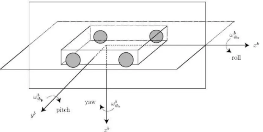
4.1.4 Body frame (b-frame)

The body frame is the coordinate system associated with the vehicle. The coordinate system has its origin at the center of gravity of the vehicle and the x-axis points in the forward direction, the

z-axis down through the vehicle and the y-axis completes the right hand coordinate system. See

Figure 4.2. This frame will be denoted by the superscript b

In some applications the instrumentation platform is not aligned with the body frame, and thus a (orthonormal) platform frame is needed as well. The platform frame is the coordinate system of the platform which the accelerometers and the gyros are mounted on.

Throughout this thesis the platform is assumed to have its coordinate axes perfectly aligned with the body coordinate axes, and therefore no distinction between the two frames will be made.

Figure 4.2: Body coordinate frame.

The inertial sensors resolves their measurements along the sensitivity axes of the instruments. The instrument sensitivity axes of the gyros and accelerometers spans the axes of the gyro and accelerometer instrumental frames, respectively. The instrumental frames can not be assumed to be orthogonal and identification of the misalignment matrices for transformation between the instrumental and platform frame is the primary objective of the IMU alignment, see [6].

(30)

4.2 Coordinate Frame Transformation

In navigation systems its often necessary to transform a vector from one coordinate system into another.

This section describes a two different methods to derive a mathematical expression for the rotation matrix relating two Cartesian, orthogonal coordinate systems.

Further, small angle rotations and derivatives of rotation matrices are studied.

4.2.1 Projection

The first method presented on how to find a mathematically expression for the rotation matrix relating to coordinate systems is based upon projections of a vector onto the orthonormal bases of the two coordinate systems.

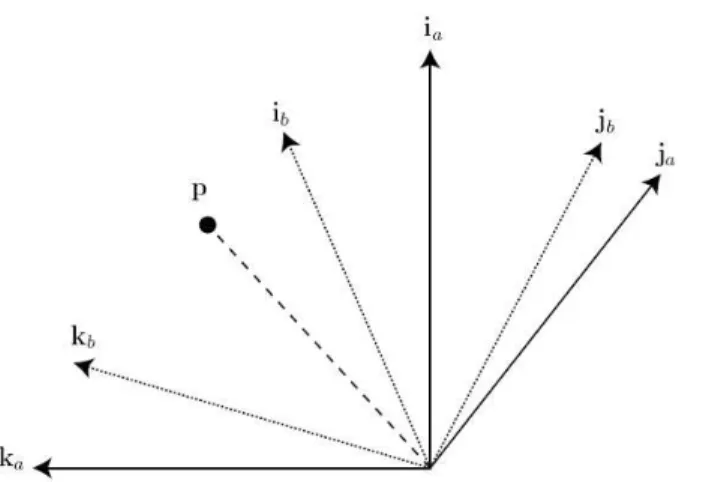
Figure 4.3: By projection of vector p onto the bases of the two orthonormal coordinate systems the

directional cosine matrix relating the two coordinate systems can be found.

Mathematically this method can be described as follows. Let: { ia ja ka } and { ib jb kb }

be the unit vectors spanning two orthonormal coordinate systems having the same origin, see Fig-ure 4.3. Vector p can then be written in terms of the unit vectors spanning coordinate system A, that is

p = xaia+ yaja+ zaka (4.1)

Projection of p onto the unit vectors spanning coordinate system B and using the fact that the bases of the coordinate system are orthogonal results in

xb=< ib, p >=< ia, ib> xa+ < ja, ib> ya+ < ka, ib> za

yb=< jb, p >=< ia, jb> xa+ < ja, jb> ya+ < ka, jb> za

zb=< kb, p >=< ia, kb> xa+ < ja, kb> ya+ < ka, kb> za

where scalar product < ik, jl>= cos (αi_k, j_l). Here αi_k, j_l denotes the angle between vector ikand jl.

In matrix form this can be written as

(31)

where

Rb_a= 

 _{cos (α}cos (α_iia,ib) cos (αja,ib) cos (αka,ib)

a, jb) cos (αja, jb) cos (αka, jb)

cos (αia,kb) cos (αja,kb) cos (αka,kb)



 _(4.3)

The rotation matrix Rb_a a is a so called Directional Cosine Matrix (DCM). Although Rb_a a has nine elements, it has only three degrees of freedom and can be uniquely described by the three Euler angles, in the sequel gathered in the vector Θ [9]. The directional cosine matrix is an orthonormal matrix, that is

Rb_aT Rb_a= Rb_aRb_aT = I3 (4.4)

Hence, the inverse of the rotation matrix is the same as its transpose.

4.2.2 Plane rotations

Plane rotations are a convenient way to mathematically express the vector transformation between two coordinate frames with common origin, where the second coordinate system can be related to the first by a rotation around a vector v. In the case of v being one of the coordinate axes the rotation matrix takes a simplified form.

The rotation matrix between two coordinate systems related by a sequences of plane rotations can be found by multiplying the plane rotation matrices in the order of the rotations.

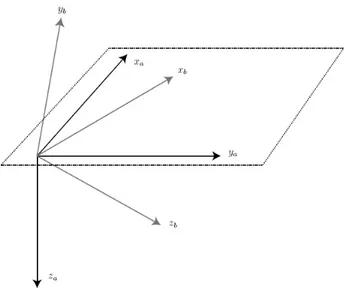
Figure 4.4: Coordinate system A and B referred to in the derivation of the rotation matrix Rb_a a through of plane rotations.

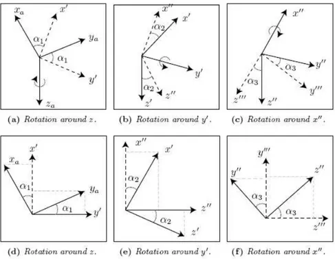
By plane rotations the directional cosine matrix relating coordinate system A and B in Figure 4.4 can be found in the following manner. First rotating coordinate system A around its z-axis with α1radians to align the new x0-axis with the projection of xb-axis onto the plane spanned by x0-axis

and the y0-axis. See Figure 4.5(a) and Figure 4.5(d). The rotation can be described as   x 0 y0 z0   = 

 _{− sin (α}cos (α1₁)_{) cos (α}sin (α1₁) 0_{) 0}

0 0 1     x_ya_a za   = R0_a   x_ya_a za   _(4.5)

(32)

Figure 4.5: Plane rotations.

Next, rotating the new coordinate system, denoted with prime with α2radians around the y0-axis,

resulting in that the x0-axis becomes aligned with the xb-axis. This is illustrated in Figure 4.5(b)

and Figure 4.5(e). The rotation is described by   x 00 y00 z00   =   cos (α₀ 2) 0 − sin (α₁ ₀ 2) sin (α2) 0 cos (α2)     x 0 y0 z0   = R00 0   x 0 y0 z0   _(4.6)

Then rotating the new coordinate system α3radians around the x00-axis results in that the y00- and

z00-axis aligns the yb- and zb-axis, respectively. See Figures 4.5(c) and 4.5(f). The last plane rotation

is described by   x_yb_b zb   =   1₀ _{cos (α}0 ₃₎ _{sin (α}0 ₃₎ 0 − sin (α3) cos (α3)     x 00 y00 z00   = Rb 00   x 00 y00 z00   _(4.7)

The rotation matrix from coordinate system A to B is found by multiplying the rotation matrices in Equations (4.5)-(4.7) in the order of rotations. The rotation matrix Rb_aa reads

Rb_a= R0_aR000 Rb00= (4.8)   −s(α1) c(αc(α3)+c(α1) c(α1) s(α2) 2) s(α3) c(α1) c(αs(α3)+s(α1) c(α1) s(α2) 2) s(α3) c(α−s(α2) s(α2)3) s(α1) s(α3)+c(α1) s(α2) c(α3) −c(α1) s(α3)+s(α1) s(α2) c(α3) c(α2) c(α3)  

Here s(·) and c(·) denotes the sine and cosine operation, respectively. The rotation matrices used throughout this thesis can be found below.

(33)

4.2.3 Rotation matrices

It is clear by now that coordinate rotations are essential parts of inertial navigation.

Throughout this report the most extensively used coordinate rotation matrix is the Navigation to Body frame rotation matrix Rb_n. It is possible to find an expression for the rotation matrix Rb_n directly in terms of the three Euler angles relating the navigation and body coordinate systems.

Rb_n= (4.9)   −s(ψ) c(φ)+c(ψ) s(θ) s(φ)c(ψ) c(θ) c(ψ) c(φ)+s(ψ) s(θ) s(φ)s(ψ) c(θ) c(θ) s(φ)−s(θ) s(ψ) s(φ)+c(ψ) s(θ) c(φ) −c(ψ) s(φ)+s(ψ) s(θ) c(φ) c(θ) c(φ)   where: φ - roll [radians] θ - pitch [radians] ψ - yaw [radians] c(·) - cosine operator s(·) - sine operator

Its also easy to find an expression for the rotation matrix Rn_e terms of geodetic coordinates.

Rn_e= (4.10)   −s(φ) c(λ)_−s(λ) −s(φ) s(λ)_c(λ) c(φ)₀ −c(φ) c(λ) −c(φ) s(λ) −s(φ)   where: φ - latitude [radians] λ - longitude [radians] c(·) - cosine operator s(·) - sine operator

4.2.4 Small angle rotation

When two coordinate systems differ only by small angles rotations the corresponding directional cosine matrix can be approximated being a linear function of the rotation angles. This is a very use-ful property in the derivation of the INS error equations and derivative calculations of the rotation matrix.

Let coordinate system A and B be differently oriented by the small angle rotations βx, βy and

βzaround the axis of system A. For small x the approximations cos(x) ≈ 1 and sin(x) ≈ x are valid

by aid of Taylor series expansion. Applying this to Equation 4.8, the small angle rotation matrix can be approximated as Rb_a≈   _−β1_z β₁z −β_β_xy βy −βx 1   = I3+ Ξβ (4.11)

(34)

where Ξ_β is the skew symmetric matrix representation of β =£ βx βy βy

¤_T

, defined such that

p × β = Ξ_βp (4.12)

Here p is an arbitrary 3 × 1 vector. The matrix Ξβ reads

Ξβ=   _−β0_z β₀z −β_β_xy βy −βx 0   _(4.13)

Using the properties of the cross product, it is straight-forward to show that Ξ_βp = −Ξpβ, where

Ξpis the skew symmetric matrix representation of the vector p.

4.3 Rotating Coordinate Frame

As the attitude of the vehicle changes, so does the relative angle between some of the coordinate frames in the navigation system. Hence, so does the rotation matrices relating this coordinate frames.

The rate of change of the rotation matrix corresponds to the first order derivative of the direc-tional cosine matrix. Assuming that angular velocity ω_baa between coordinate system A and B is constant in the interval t to t + ∆t, then using the result from small angles rotations the rotation matrix at time t + ∆t can be written as

Rb_a(t + ∆t) = Rb_a(t) [I3+ Ωaba(t) ∆t] (4.14)

where Ωa_ba ba is the skew symmetric matrix representation of the angular rates ω_baa . The matrix Ωa ba reads Ωa_ba=   0 −ωa_ba,z ωa_ba,y ωa_ba,z 0 −ωa_ba,x −ωa_ba,y ωa_ba,x 0   _(4.15)

and the rotations ωa_ba,x, ωa_ba,y and ωa_ba,z correspond to rotations about the x, y and z axes, respec-tively, of the a-frame with respect to the b-frame coordinated with the a-frame. Using the definition of derivative, the rate of change in the rotation matrix becomes

˙ Rb_a(t) = lim ∆t→0 Rb_a(t + ∆t) − Rb_a(t) ∆t = lim ∆t→0 Rb_a(t)£I3+ Ωa_ba(t) ∆t ¤ − Rb_a(t) ∆t = Rb_a(t) Ωa_ba(t) (4.16) where (4.14) was used in the second equality. Not surprisingly the rate of change of the rotation matrix is a function of both the current orientation and the angular rate between the coordinate systems. The transposed equivalent is

˙ Ra_b(t) = h Rb_a(t) Ωa_ba(t) i_T = Ωa_ba(t)TRa_b(t) = −Ωa_ba(t) Ra_b(t) (4.17)

(35)

The skew symmetric rotation matrix in Equation (4.15), coordinated in one frame, can be related to a rotation matrix coordinated in another frame by using the similarity transformation

Ωb_ba= Rb_aΩa_baRa_b (4.18) Note that the sense of the rotation, i.e. a relative to b, is unchanged.

(36)

Chapter 5 Inertial Navigation Equations

In this chapter the fundamental equation of inertial navigation is derived. Further, the n-frame navigation equations are introduced and the physical interpretation and significance of the different terms are discussed.

By mechanization of the n-frame navigation equations a linear model of how the sensor errors are related to the errors in the navigation output is found. The linear error model will later be used in the integration between the INS and GPS-receiver.

A discrete time ZOH version of navigation equations and error equations will be presented.

5.1 Fundamental Equations of Inertial Navigation

According to Newtons first law of motion an object tends to keep its initial speed and attitude unless affected by an unbalanced force. Hence, a change in motion is a result of a force being applied to overcome the objects inertia. Two types of forces determine the motion of a vehicle: gravity and inertial force.

5.1.1 Gravity force

Newtons universal law of gravity states that the force fg , due to gravitational attraction between

two masses m1and m2, see Figure 5.1 is

fg= G m1m2

|r|3 r (5.1)

where G denotes the universal gravity constant and r the position vector of mass m2with respect

to the center of mass m1 . Let mass m1be equal to the earth mass M and m2equal to the vehicle

mass m. Assuming the vehicle is at a far distance from the earth, then the vehicle sensed gravity force becomes

fg= −G M m

|r|3 r (5.2)

Rewriting this as force per vehicle unit mass yields g ,fg

m = −

G M

|r|3 r (5.3)

(37)

Figure 5.1: Gravity attraction between two masses m1and m2at the distance r from each other.

5.1.2 Inertial force

Newton’s second law states that the acceleration of an object is directly proportional to the magni-tude of the net force, in the same direction as the net force and inversely proportional to the mass of the object. In the case the inertial force being the only force acting upon the vehicle

fI = m s (5.4)

Here fI is the inertial force applied to the vehicle of mass m to produce the acceleration s. The

acceleration s will henceforth be refereed to as the specific force.

5.1.3 Equations of motion

In the previous sections the kinematic equations for an object were derived in the absent of either the inertial force fI or the gravity force fg. In reality the motion of an object is mostly a result of

both these forces being present.

The total force, ftotacting upon the object can be expressed as the sum of the gravitational and

inertial force, that is

ftot= fg+ fI (5.5)

Substituting the left hand side with the kinematic acceleration in the i-frame times the mass m of the vehicle gives

m ¨ri= fg+ fI (5.6)

Replacing the right hand side of (5.6) with (5.2) and (5.4) gives

m ¨ri= −G M m

|ri_|3 r

i_{+ m s}i _(5.7)

Finally the fundamental equation of inertial navigation is obtained by dividing with the mass m on both sides, resulting in

¨ri= gi+ si (5.8) The equation states that the kinematic acceleration ¨ri_{is equal to the sum of the gravity acceleration}

(38)

5.2 Navigation Equations

The navigation equations are a set of differential equations describing the relationship between the INS outputs (that is velocity, position and attitude) and the inputs in terms of acceleration and angular rates.

In this section we will derive the navigation equations for a Strap-down inertial system. There are several mechanizations that are used in practice, each being chosen based on the type of appli-cation that the vehicle is used for. The Local Level mechanization frame will be used.

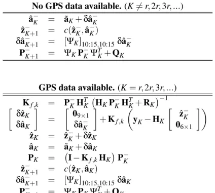
Figure 5.2: Functional diagram of a Strap-Down INU.

The navigation frame mechanization provides vehicle ground speed and attitude data with re-spect to a Local Vertical Local Horizontal frame, which is consistently orientated in the same pointing directions with respect to the ground plane and the local gravity direction, wherever the vehicle navigates around the globe. This is useful for most on-board guidance systems, which control the vehicle with respect to the local ground plane.

The resulting differential equations are nonlinear and will be formed in terms of measured accelerations and angular rates, rather than standard Newtonian form.

In order to integrate the INU with independent Kalman Filter data, a linearization of the equa-tions is necessary, and error sources will be described. Note that linearization can be performed in different ways, depending upon the application and also on the industrial proprietary capabilities of INU makers.

A general block diagram of a Strap-down INU is shown in Figure 5.2. The core of the INU is a set of 3 gyros and 3 accelerometers mounted in orthogonal triads and rigidly attached to the vehicle. The gyros sense the motion ω_ibb in body-fixed coordinates. The accelerometers output sb is transformed into the navigation frame by the navigation computer using Rn_b, which is generated in the computer by the body rates coming from the gyros, and the navigation frame rates created by the vehicles velocity.

(39)

5.2.1 Velocity equations

The velocity vector vn=£ vnorth veast vdown

¤_T

in the rotating navigation frame is given by the position rate of change in ECEF frame as

vn= Rn_e˙re (5.9) Taking the time derivative

˙vn= ˙Rn_e˙re+ Rn_e¨re (5.10) The position vector and its derivative, related to the inertial frame are

re = Re_iri

˙re = ˙Re_iri+ Re_i ˙ri = Re_i(˙ri− Ωi_ieri) ˙

Re_i = −Re_iΩi_ie (5.11) Taking the second time derivative of reresults, after some algebra, in

¨re = Re_i(¨ri− Ωi_ie˙ri− ˙Ω_iei ri) + ˙Re_i(˙ri− Ωi_ieri) = Re_i(¨ri− Ωi_ie˙ri) − R_ieΩi_ie(˙ri− Ωi_ieri)

= Re_i(¨ri− 2 Ωi_ie˙ri+ Ωi_ieΩi_ieri) (5.12)

where the Earth’s rotation rate is assumed to be constant at one revolution per day, or ˙

Ωi_ie= 03×3 (5.13)

The time rate of change of the direction cosine matrix Rn_e is ˙

Rn_e = −Ωn_enRn_e (5.14) Substituting Equations (5.11), (5.12) and (5.14) into equation (5.10) yields

˙vn = Rn_eRe_i(¨ri− 2 Ωi_ie˙ri+ Ω_iei Ωi_ieri) − Ω_enn Rn_eRe_nvn

= Rn_i (¨ri− 2 Ωi_ieRi_nvn− 2 Ωi_ieΩi_ieri+ Ωi_ieΩi_ieri) − Ωn_envn = Rn_i (¨ri− 2 Ωi_ieRi_nvn− Ωi_ieΩi_ieri) − Rn_i Ωi_enRi_nvn

= Rn_i [¨ri− (Ωi_en+ 2 Ωi_ie) R_ni vn− Ωi_ieΩi_ieri] (5.15) where, in the second step in this equation, the following relationship is used

˙ri= Ωi_ieri+ Ri_nvn (5.16) The specific force sn_{is the sensed output of accelerometers coordinated in the navigation frame.}

The specific force is a combination of inertial and gravitational contributes

sn= Rn_i ¨ri− Gn (5.17) Gravitational acceleration includes gravity and centripetal acceleration induced by Earth’s rotation, see Appendix A:

(40)

Using

Ωn_ieΩn_ie= Rn_i Ωi_ieRi_nRn_iΩi_ieRi_n (5.19) and combining Equations (5.17)-(5.18) and rearranging terms yields

¨ri = Ri_n(sn+ Gn)

= Ri_n(sn+ gn+ Rn_i Ωi_ieΩi_ieRi_nrn)

= Ri_n(sn+ gn) + Ωi_ieΩi_ieri (5.20) Substituting Equation (5.20) into Equation (5.15) yields

˙vn = Rn_i [Ri_n(sn+ gn) − (Ωi_en+ 2 Ωi_ie) Ri_nvn] = sn+ gn− Rn_i (Ω_eni + 2 Ωi_ie) Ri_nvn (5.21) or ˙vn = sn− (Ωn_en+ 2 Ωn_ie) vn+ gn = sn− (ω_enn + 2 ω_ien) × vn+ gn (5.22) where sn = Rn_bsb gn = £ 0 0 g ¤ (5.23) Ωn

enand Ωnieare the skew symmetric matrices obtained from ωenn and ωien, respectively. This

equa-tion gives the basic descripequa-tion of velocity change in a local level navigaequa-tion frame; it is directly applicable to either Gimballed or Strap-down mechanizations.

5.2.2 Position equations

For an easy integration with GPS measurements, the position vector will expressed in terms of

Latitude, Longitude and Height. For position rates it’s necessary to introduce an Earth model and

it’s geometry.

Like reference frames definition, there are many models for Earth’s geometry. These models are based on parameters that have been assigned different values for different uses. For integrated navigation systems, the Earth’s shape is modeled by simple oblate spheroid.

The local geodetic frame is to be maintained as locally level as a vehicle moves over the Earth’s surface. This movement results in an angular rotation defined dy the Earth’s geometrical shape, i.e., it’s radius of curvature. Integration of this motion yields the vehicle position. An accurate model of the Earth’s shape is necessary so that an accurate position results from the integration.

Motion over the surface of the ellipsoid is along the arch defining the surface. The rate of change of latitude is along the meridian and is governed by the curvature along this arc as

˙φ = vnorth

Rm+ h (5.24)

The rate of change of longitude is found from

˙λ = veast

(41)

Height rate will be assumed as directly dependent from vdown

˙h = −vdown (5.26)

Rm and Rn are the Meridian and Normal radii of curvature; along the lines of constant longitude

and latitude respectively. Their analytical definition is given in Appendix A.

5.2.3 Attitude equations

The attitude equations are based on the gyros output. With reference to Equation (4.17), the rate of change of the DCM matrix is given by

˙

Rn_b= −Ωn_bnRn_b (5.27) Where the skew symmetric matrix Ωn

bnis formed from the rotation vector ωbnn as

Ωn_bn=   0 −ωn_bn,3 ωn_bn,2 ωn_bn,3 0 −ωn_bn,1 −ωn_bn,2 ωn_bn,1 0   _(5.28)

The rotation vector is obtained from the gyros measurements ωb_ibas

ω_bnn = ω_inn − Rn_bω_ibb (5.29) where ωn_in= ωn_en+ ω_ien (5.30) ωn_en=£ veast Rn+h − vnorth Rm+h − veast Rn+h tan(φ) ¤T (5.31) ω_ien =£ Ω cos(φ) 0 −Ω sin(φ) ¤T (5.32) Where Ω = 7.292115e−5rad/s is the Earths turn rate. Time evolution (solution) of (5.27) with

(5.29) can be performed in several ways

• Integration of 6 DCM elements and computation of the other 3. • Integration of 4 Quaternions.

• Integration of (5.27) directly

All techniques require initialization. In this thesis, third method will be used.

5.3 Perturbation Equations and Errors

The nonlinear navigation equations are now linearized to obtain linear error models. The error system provides a useful way to study INS error propagation using linear methods and as the basis for designing Kalman filters to implement the various aiding techniques.

We need an error model in order to determine how the computed velocity, position and attitude deviate from true values. These deviations are mainly due to Accelerometers and Gyros errors, and Initial condition errors. Linearization is performed as perturbation on velocity, position and attitude.