Analytical Model for out-of-plane mechanical behaviour

Analytical Model for out-of-plane

mechanical behaviour

5.1 Overview

As is already the case for reinforced concrete, steel and wood constructions, in

designing masonry structures, it would be useful for designers to know the

crushing domains, N–e (axial force–eccentricity) or M–N (bending moment–axial

force), which enable rapid calculation of the bearing capacity of a wall with preset

exposure times to fire. The method proposed herein aims to define such M–N

diagrams for walls subjected to the eccentric axial force acting on various types of

blocks masonry exposed to fire on one side. To this end, the temperature

distributions across the wall thickness are first determined. Then, as the laws

governing the decay of the material strength and axial stiffness as a function of the

of the curvature. Lastly, based on the isotherms already calculated and the stress–

strain–temperature constitutive relation, we determine the crushing surfaces on the

plane N–e (in which e is the out-of-plane eccentricity and N is the axial force) for

increasing exposure time to nominal fire. Application of the procedure is

illustrated through a simple example.

5.2 Thermal analysis

We shall refer to a wall of height h, thickness t and unit depth, subjected to a

thermal transient due to a heat source acting on one side.

The convective thermal action in terms of net unitary heat flow is:

, ( ) 2 net c c g m W h m         _{ }  , (5.1)

where Θm is the element’s surface temperature [°C], while the temperature Θg of

the gases produced by fire is determined via the expression for the nominal

temperature–time curve (2.7).

The heat transmission coefficient for convection αc has been taken as 25 W/m2K,

as indicated in EN 1991-1-2 [33].

The net unitary heat flow due to irradiation is:



 



with the emissivity εf = 1.0 and temperature Θr tied to the normalized curve (2.7).

value for the receiving surface, εm, has been set to 0.8, as recommended in EN

1991-1-2 [33]. The configuration coefficient Φ has been assumed equal to 1.

The nonlinear thermal transitory was analysed via the code ANSYS Multiphysics

rel. 11.0 using triangular (or quadrangular) shaped plane elements (PLANE55 “2-D Thermal Solid”) of dimensions varying from 1 to 2 cm.

The initial temperature was 20°C, while a unit convective thermal flow was

applied to the surface not exposed to the fire, using a transmission coefficient αc

of 4 W/m2K. The functions for specific heat ca(T) and transmissibility λa(T) have

been drawn from Appendix D of EN 1996-1-2 [1], as shown in Fig. 5.1 (brick with

density =1000 kg/m3) and Fig. 5.2 (lightweight aggregate concrete with density

= 800 kg/m3).

The results of such analyses of the nonlinear thermal transitory are presented in

the plots of temperature T versus the thickness x for various exposure times to

nominal fire (Figures 5.3 and 5.4).

0.00 1.50 3.00 4.50 6.00 7.50 9.00 0.00E+00 2.00E+04 4.00E+04 6.00E+04 8.00E+04 1.00E+05 1.20E+05 0 200 400 600 800 1000 1200 1400 ca (T ) [d aN ∙c m /( k g° C )] λa [d a N /( m in °C )] T [°C] ca(T) λa(T)

Fig. 5.1: Thermal conductivity λa(T) [daN/min°C] and specific heat ca(T) [daN·cm/kg°C] functions adopted

Fig. 5.2: Thermal conductivity λa(T) [daN/min°C] and specific heat ca(T) [daN·cm/kg°C] functions adopted

for the lightweight concrete blocks.

0 200 400 600 800 1000 1200 0 5 10 15 20 25 30 35 T _[°C] x [cm] 30 min 60 min 90 min 120 min 150 min 180 min Limit Temperature θ2

Fig. 5.3: Brick wall: temperature profile for various exposure times. The value of θ2 (the temperature beyond

which the material is to be considered ineffective) is indicated at 600°C, as per Appendix C of EN 1996-1-2 [1].

0 200 400 600 800 1000 1200 0 5 10 15 20 25 30 35 T _[°C] x [cm] 30 min 60 min 90 min 120 min 150 min 180 min Limit Temperature θ2

Fig. 5.4: Lightweight aggregate concrete masonry wall: temperature profile for various exposure times. The

value of θ2 (the temperature beyond which the material is to be considered ineffective) is indicated at 400°C,

as per Appendix C of EN 1996-1-2 [1].

The same procedure has also been performed on a panel of aerated autoclaved

concrete (AAC) blocks to obtain numerical results for a comparison with a set of

experimental data.

5.3 Mechanical analysis

5.3.1 Description of the mathematical model and basic hypotheses

In the model, failure of the masonry is associated with the attainment of crushing

strain conditions in some point of a generic cross section. The basic underlying

hypotheses are the following:

 cross sections remain planar (Bernoulli-Navier hypothesis);

 the material responds to the “Maximum strain” yield criterion.

In order to simplify the analysis, it has also been considered that thermal strain εth,

transient strain εtr and slenderness effects are formally computed increasing the

applied stress.

Referring to the quantities indicated in Fig. 5.5, with a fixed exposure time to the

nominal fire, the results of the thermal analyses lead to the following function for

the temperature profile:

 

Fig. 5.5: Horizontal cross section of the wall; the geometric parameters are indicated, together with a diagram

of the crushing strain diagram εu(x).

The term X is the abscissa with its origin on the face exposed to fire, x is the

abscissa whose origin lies on the border of the effectively resistant section, tineff is

the depth of the portion of wall deemed ineffective, tFr is the thickness of the still

reacting part, and t is the total thickness of the wall itself. By placing:

ineff ineff X x t x X t        , (5.4)

the value of the temperature T as a function of x can be obtained:

 

T T x . (5.5)

By observing the behaviour of the resistance fcu(T), the elasticity modulus E(T)

and the crushing strain u), from Fig. 5.5, it follows immediately that:

 

 

 

For this last equation, we assume, where definable, the condition:

2 2 0 u x   _  . (5.9)

The distributions ε(x) vary within five limit fields, as illustrated in Fig. 5.6, where

tθ1 indicates the thickness of the part between the unexposed face and isotherm θ1

(limit temperature for material integrity) and tθ2 the portion whose temperature

varies between θ1 itself and θ2 (limit temperature for material ineffectiveness),

t t x X Fr u(x) A C D B 5 4 3 2 1 t1 t2 tineff. x 

Fig. 5.6: Limit ε fields.

5.3.1.1 Field 1

Field 1 (Fig. 5.7) represents the subset of the sheaf of straight lines at point





A  , (5.10)

whose directive coefficient χ, or section curvature, belongs to the following

domain:

 

and which is defined by





 

t t x X Fr u(x) A C D B t1 t2 tineff. x x x ₁ x  Fig. 5.7: Field 1.

By means of the constitutive relation, the function of the normal stress σ(x)

through the thickness, which, in the compressed zone, equals:













 

 x    x   x _ x  _, (5.13)

while in the tensile zone,





 

 x    x _x  t_Fr_. (5.14)

In previous expressions, x1 denotes the following function:

 

 

 

 

5.3.1.2 Field 2

Field 2 represents the subset of the straight lines tangential to the curve in Fig. 5.8,

in which χ varies within the following existence field:

 





 

where x is the generic abscissa of wall thickness belonging to the domain:





The equation of the straight lines in this field is:





 





 

From the constitutive relation, the normal stresses σ(x) in the compressed zone













 

 x x   x x  x _ x x _, (5.19)

while in the tensile zone,





 

 x x   x _x x tFr_. (5.20)

In the previous expressions, x2 denotes

 

 

 

 

 





 

 





Field 3 (Fig. 5.9) accounts for the possibility that the function εu(x) not be

derivable at the point C whose coordinates are:





C t_ ;_u(t_ ) . (5.22)

Such a field only exists under the aforementioned condition or in the event that

the entire section is at a temperature above θ1, which would imply that

1 0

t_  ; (5.23)

otherwise, we proceed directly to examination of Field 4.

Bearing in mind the foregoing premises, Field 3 is the subset of the sheaf of

straight lines at point C where χ falls within the interval:





 

and whose equation is:









 

The normal stresses σ(x) in the compressed zone are:













 

 x    x   x _ x  _, (5.26)

while in the tensile zone,





 

 x    x _x  tFr_. (5.27)

In the preceding expressions, x3 indicates the following function:

 

 

 

 

5.3.1.4 Field 4

Field 4 (Fig. 5.10) represents the subset of the sheaf of straight lines of the point:





D t_Fr;_u(t_Fr) , (5.29)

whose directive coefficient χ falls within the following interval:

 

and whose equation is:









 

The normal stresses σ(x) within the thickness are:

















5.3.1.5 Field 5

Field 5 (Fig. 5.11) represents the subset of the sheaf of straight lines of point D

whose coordinates are given by equation (5.29), whose directive coefficient χ falls

within the following interval:

 

and whose equation is still (5.31).

t t x X Fr u(x) A C D B 5 t1 t2 tineff. x x x x x  Fig. 5.11: Field 5.

The normal stresses σ(x) in the compressed zone are:













 

 x    x    x _x  t_Fr, (5.34)

while in the tensile zone,





 

 x     x _ x  _. (5.35)

 

 

5.3.1.6 Definition of the M–N crushing domain

By integration, we obtain the curvature functions Nu(χ) and Mu(χ) for fields 1, 3, 4

and 5 via equations (5.37) and (5.38), and the functions for the generic abscissa

through the thickness, Nu(x ) and Mu(x ) for field 2 via equations (5.39) and

(5.40). Therefore, the boundary points of the resistance domain M–N can be

determined for any given value of χ or x :

 







 







 







 

 



The integration extremes a and b in the preceding expressions are indicated in

Field a b 1 0 x1() 2 0 x2(x ) 3 0 x3() 4 0 tFr 5 x5() tFr

Tab. 5.1: Integration extremes in relations (5.37), (5.38), (5.39) and (5.40).

5.3.2 Adaptation of the model to particular cases

The model described above is valid only in the case where the condition (5.9) is

satisfied. However, with an appropriate correction it can also be extended to the

case where we have:

2 2 0 u x   _  , (5.41)

which physically occurs when the function T(x) has an inflection point in the

thickness. The procedure consists in replacing the portion of the curve εu(x),

greater than that which we have the condition (5.41), with a straight line, which is

the unique arrangement of the ε belonged to the Field 2 in which the crash

situation occurs simultaneously in the two points x1* e x2* (Figure 5.12). The

determination of this strain arrangement is obtainable putting:

 

 

t t x X Fr A C D B 2 t1 t2 tineff. x  correct(x) original (x) x x   u u

Fig. 0.12: Procedure for correcting the εu(x) function for the model adaptation.

5.3.3 Application of the model and presentation of results 5.3.3.1 Lightweight aggregate concrete

The temperature profiles across the thickness were determined by preliminary

thermal analyses (Fig. 5.4). Therefore, by then changing the reference system,

through equations (5.4) and (5.5), we were able to define relations (5.6), (5.7) and

(5.8).

With reference to the stress–strain curves reported in Annex D of EN 1996-1-2 [1]

(Fig. 2.27) and to those proposed in the paragraph 4.8.4.3 (Figures 4.24, 4.25,

4.26, 4.27, 4.28 and 4.29), and applying the procedure formulated above, we

determined the N–e crushing domains (per unit length) for different values of total

wall thickness and exposure time to the nominal fire.

In the Figures 5.13, 5.14, 5.15 and 5.16 the domains obtained respectively for

Eurocode, LWC, LWC-LAP and LWC-FV constitutive laws are shown for wall

implementation (Fig. 5.13), the rule of neglecting the inefficient part of the wall at

a temperature higher than 400°C (see Table 2.8) was adopted, because this is not

detected in the experimental data presented in the paragraph 4.4 for each

lightweight concrete material tested. In this sense the Eurocode gives anyway

lower values of the axial force resistance, especially for positive eccentricities

(closer to exposed side).

In the Figures 5.17, 5.18 and 5.19, a comparison between the domains obtained

with the adoption of each constitutive law are presented for various thicknesses.

The maximum reduction in terms of axial force resistance is detected in the case

of Eurocode model adoption: it goes from about 20% corresponding to a wall

thickness of 25cm exposed to nominal fire for 30 minutes, to more than 65% for a

thickness of 15cm and 180 minutes of exposure.

The material which gives the best mechanical performance when subjected to

nominal fire action is the LWC-FV: reductions in axial force strength are less than

20% (180 minutes of exposure) and are detected only for eccentricity belonging to

the range ±10% of the total thickness, as shown in the Figure 5.16, while for

higher values the differences with the mechanical strength in cold condition may

be neglected.

The LWC-LAP material shows better performances than those offered by LWC

for positive values of the eccentricity. For centred axial force condition, the

maximum reductions in strength are respectively about 25% and 40%,

Fig. 5.13: N–e crushing domains for EN 1996-1-2 constitutive law and different values of wall thickness.

Fig. 5.15: N–e crushing domains for LWC-LAP constitutive law and different values of wall thickness.

Fig. 5.17: Wall thickness of 15cm: N–e crushing domains for each constitutive law and different values of

Fig. 5.18: Wall thickness of 20cm: N–e crushing domains for each constitutive law and different values of

Fig. 5.19: Wall thickness of 25cm: N–e crushing domains for each constitutive law and different values of

5.3.3.2 Clay

By referring to the stress–strain curves reported in Annex D of EN 1996-1-2 [1]

(Fig. 2.23), it can be seen that the constitutive relation prescribed for brick is of

the limited linear-elastic type, according to the proposed one in the paragraph

4.8.4.1 with the expression (4.27).

N–e crushing domains (per unit length) obtained applying the procedure presented

above for different values of total wall thickness and exposure time to the nominal

fire are shown in the Figures 5.20 and 5.21.

As for lightweight aggregate concrete, the rule of considering as inefficient the

part of the section with a temperature higher than 600°C (Table 2.8) was adopted

only for the application to the constitutive law provided by the Eurocode.

The highest reductions in axial strength value with exposure time increasing for

Eurocode curves are about 75÷80%: this is due not only for the provided

reduction gradient for compressive strength but especially for the low value

prescribed for θ2.

The increasing in ultimate strain with temperature detected experimentally does

not produce any noticeable reduction in axial strength regardless the eccentricity

values when the proposed model is adopted. This confirms the good performance

detected with TEST 3 ‒ HMC carried out on CLAY samples.

The comparison between the domains obtained for these two different groups of

Fig. 5.20: N–e crushing domains for EN 1996-1-2 constitutive law and different values of wall thickness.

Fig. 5.22: Wall thickness of 15cm: N–e crushing domains for each constitutive law and different values of

Fig. 5.23: Wall thickness of 20cm: N–e crushing domains for each constitutive law and different values of

Fig. 5.24: Wall thickness of 25cm: N–e crushing domains for each constitutive law and different values of

exposure time to nominal fire.

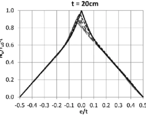
5.3.3.3 Aerated Autoclaved Concrete (AAC)

A tested masonry panel of dimensions 11.5 × 100 × 300 cm has been examined. A

comparison of the previous calculus procedure against simple compression tests

Test Utilization Factor α Exp. Time [min] Axial Force by Hahn et al. [19] [kN/m] Axial Force Calculated [kN/m] Est. Error [%] 1 – fu(20°C) = 4.01 MPa 1.0 57 230 265 -15.2 2 – fu(20°C) = 4.01 MPa 0.6 64 138 160 -15.9 3 – fu(20°C) = 4.61 MPa 1.0 48 414 317 23.4 4 – fu(20°C) = 4.61 MPa 0.6 57 253 183 27.7

Tab. 5.2: Comparison of the proposed calculus procedure against experimental results by Hahn et al. [19].

5.3.4 Example application of the model to a load-bearing wall of a hospital

Hospitals are subject to special regulations, amongst which is the Italian

Ministerial Decree of September 18th, 2002 [54], which prescribes an R120

resistance class for such structures.

Let us consider a masonry wall made of lightweight aggregate concrete blocks

(Fig. 5.25), with the cold mechanical and thermal properties reported in Table 5.3.

25 y

200

x

Mechanical and thermal properties Value

Density  800 kg/m3

Conductivity λa 0.21 W/m°C

Specific heat ca 1170 J/kg°C

Ultimate stress fu 50 daN/cm

2

Ultimate deformation εu 2.5 ‰

Elasticity modulus E 28000 daN/cm2

Table 5.3: Cold mechanical and thermal properties.

The per-unit-length values considered for axial force and out-of-plane bending

moment acting on any given transverse section have been drawn from the analysis

results and are reported in Table 5.4.

Description Characteristic Axial Force Nk [kN/cm] Characteristic Bending Moment Mxk [kN·cm/cm]

Structural element self-weight G1 3.00 4.00

Non-structural element self-weight G2 1.00 2.00

Variable overload (Cat. C) Qk 2.00 4.00

Table 5.4: Characteristic values of axial force and out-of-plane bending moment.

From the combination for exceptional actions (2.8) or (2.9), according to EN 1990

[24], we obtain: 3 1 0.6 2 5.20 / Ed N      kN cm (5.43) , 4 2 0.6 4 8.40 x Ed M      kN (5.44)

At this point, referring to Fig. 5.13 (crushing domains of a 25 cm thick wall for

various exposure times to nominal fire) and considering the plane M–N instead of

N–e, we select the curve for 120 minutes related to EN 1996-1-2 [1] and check

that it contains the point with coordinates (5.20 kN/cm; 8.40kN), as shown in Fig.

5.26. -40.00 -30.00 -20.00 -10.00 0.00 10.00 20.00 0.00 2.00 4.00 6.00 8.00 10.00 12.00 Nu [kN/cm] Mu [kN cm/cm ] 120 min Acting Forces 1.29 kN cm/cm 6.00 kN

Fig. 5.26: Assessment of fire resistance by means of domain M–N.

It can be seen that the assessment is satisfied and that the residual available

moment, Mx,Res, equals 6.00 kN·cm/cm. Hence, under the hypothesis of a 400 cm

high wall, free to rotate at its extremities, the maximum horizontal pressure qx that

may be exerted by the gases produced by the fire is given by:

,Re 2 2 2 8 8 600 200 0.03 200 400 x s x M l daN q l h cm          . (5.45)

5.4 Final remarks

Observing the different domains for the lightweight aggregate concrete units and

the brick masonry walls, it can be seen that increasing the exposure time causes

the curves delimiting the borders to intersect each other, signifying that the walls

in question do indeed improve their performance at higher temperatures.

However, such improvement is in part fictitious, in that the resisting moment

associated to each limit field has been calculated via the rotational equilibrium of

the original section around the barycentric axis, and the stress characteristics at

ambient temperature are also determined with respect to this same original

section. In fact, given equal axial force, as the exposure time progressively

increases, the resistant part of the section becomes ever smaller, with a consequent

increase in the eccentricity.

In case of adoption of Eurocode 6 constitutive law and assuming the presence of

an inefficient part over a prescribed limit of temperature, the choice of referring to

a barycentric axis of the original section for calculation of the bending moments

was dictated by our aim of simplifying the verification procedures to be carried

out by an eventual user, who would thereby be free to insert into the graphs the

values of the actions calculated via the usual methods of the mechanical analysis