8. Resource
Allocation
Call Admission Control (CAC) is the procedure employed by a node to check whether there are
sufficient resources to admit a traffic flow over one link. The procedure is the same during the PATH or RSV phase, for the downstream or upstream link.
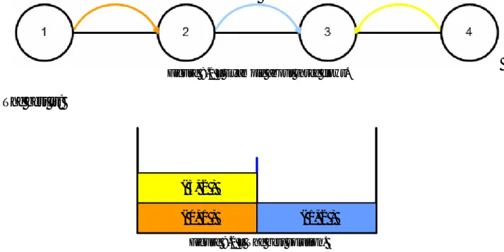
For allocate resources a random selection of slots is not the best choice. For example, if there are four nodes with chain topology and three flows: • node 0 – node 1
• node 3 – node 2 • node 1 – node 2
These are allocated in this order; I can have 0-1 and 3-2 at the same time (spatial reuse).
Figure 8.1 – Example about three flows.
The best is:
( 0, 1 ) ( 3, 2 )
( 1, 2 ) Figure 8.2 – The best solution.
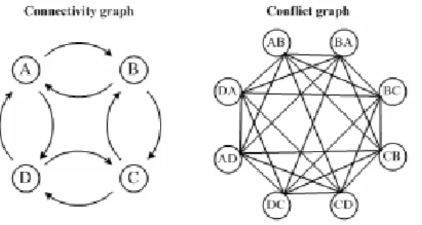
If there are 0-1 and 3-2 in two different minislots there is not spatial reuse because it is impossible to transmit 1-2 at the same time by 0-1 or 3-2
( 0, 1 ) ( 3, 2 ) Figure 8.3 – Solution without spatial reuse.
The main idea is to partition the data sub-frame into a number of groups of equal size. Each link of the network is then assigned to one of these groups in a distributed manner by all nodes.
Minislots_per_group= ⎥ ⎦ ⎥ ⎢ ⎣ ⎢ _groups number_of_ _per_frame _minislots number_of_
In IEEE 802.16 a (logical) link is set up between two nodes by means of a link establishment procedure, provided that they can communicate directly with each other, i.e. they are in the transmission range of one another.
Each group is built so that all the links that belong to it can be activated simultaneously, i.e. simultaneous transmissions on the links of the same group can be successfully decoded by the receivers. Therefore, any node of the network can allocate resources for one of its links independently of one another.
The following two issues should be considered.
• It is pretty obvious that all nodes must use the same algorithm to compute the groups over the same input data, so as to obtain a consistent group allocation, since in general, many different group partitioning can be envisaged from the same link set. In any case, this requires network-wide information to be distributed among all the nodes. This activity might be performed by the routing protocol, provided that the data required to build the groups are piggybacked on the routing messages. Note that the IEEE 802.16 standard does not specify any mandatory protocol to be used for routing.
• Most critical issue is how to state that any two links interfere with one another when activated simultaneously. This problem is regarded as one of the most important open issues of WMNs, and is still under investigation, while some preliminary works have been published in the literature [7]. Since the focus of this work is the bandwidth reservation protocol, I solved this issue in a simplistic manner with the following protocol model.
Two links can belong to the same group if: The source is different from the source.
The destination is different from the destination The source is different from the destination. The destination is different from the source The source is not a neighbour of the destination The destination is not a neighbour of the source
The total interference caused by the nodes lying outside the one-hop neighborhood of the receiving node is assumed to be negligible.
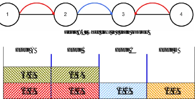
Each node only needs to know the set of links to any of its neighbors. Based on that, it is straightforward to derive in a distributed manner the connectivity graph of the network and its relative conflict graph, which are widely used means to represent the network topology and to characterize the link interference, respectively. In the former vertices represent nodes of the network and edges links. In the latter vertices represent links and edges mutual interference. Note that links need be sorted according to any non-ambiguous criterion (e.g. lexicographically) in order for the conflict graph to be the same for all nodes.
An example of connectivity and conflict graph is show in Figure 8.4.
8.1
Building of the Groups
After the conflict graph has been computed, each node must use the same algorithm to partition the links into groups. Note that having as few groups as possible is a desirable condition, since this leads to having more slots for each link, i.e. higher capacity for traffic flows.
Unfortunately, finding the minimum number of groups required finding the maximum independent set of the conflict graph. It is worth noting that, in practice, the interference among links can change over time, due to the time-varying properties of the wireless channel. Whenever this happens, the links need be re-partitioned into a new set of groups, which makes it impractical to use exhaustive search algorithms in most WMN deployments. However, several heuristics are present in the literature of graph theory [4] and WMNs [22]. Furthermore, since nodes in WMNs are usually assumed to be fixed, the link quality and the interference conditions can be considered stable for reasonably long periods of time. This considerably reduces the chance of re-computing the set of groups. The selection of the “best” heuristic algorithm, e.g. in terms of the time required to find a fractional sub-optimum solution, and, in general, the adoption of more sophisticated techniques to characterize the interference and to calculate the groups are not considered in this study and left for future investigation.
I use two different algorithms to compute the groups:
• Optimum: the groups are calculated through the maximum clique. Through optimum algorithm the number of groups is the smallest possible.
• Heuristic: each node builds the groups independently from the other nodes. The nodes are recognized by the node ID, and are organized with increasing node ID. The nodes know the network topology and the links between them.
Heuristic algorithm follows the next steps:
1. Each node takes the first link about the first node, creates a group and inserts the link in this group, then takes the second link about the first node, creates a group and inserts the link in this second group; the same for the other links about the first node.
2. Each node takes the first link about the second node and checks if this can be inserted in the last group created through the step one, otherwise checks the other groups from the last created to the first created. If the link cannot be inserted in any group, the node creates a new group.
8.1.1 Heuristic Algorithm Example
Figure 8.5 – Chain topology.
Links: • (0 1) • (1 0) (1 2) • (2 1) (2 3) • (3 2) Steps: 1. group A: (0,1) 2. group B: (1,0) 3. group C: (1,2) 4. group D: (2,1) 5. group B: (1,0) (2,3) 6. group A: (0,1) (3,2) At the end, I achieve: • Group A: (0,1) (3,2) • Group B: (1,0) (2,3) • Group C: (1,2) • Group D: (2,1)
In this example I have four minislots for each frame, one for each group.
Figure 8.6 – Three flows in a chain topology.
(1, 2)
(3, 2)
(0, 1)
Group A Group B Group C Group D
(1, 0)
(2, 3)
(2, 1)
8.2
Comparison among Heuristic and Optimum Algorithm
I want to estimate what algorithm is best for:• Graph colouring.
• The resources used through the access to the conflicts matrix. This evaluation is made through three topologies:
• Grid. • Multiring. • Bintree.
8.2.1 Grid
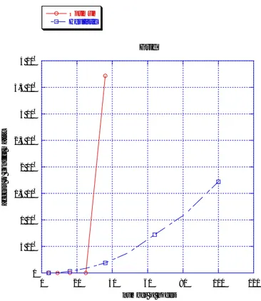
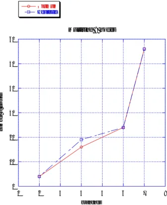
I have analyzed grid topology from 4 to 100 nodes. The number of groups with optimum algorithm is better, but the complexity is exponential, so for grids with more than thirty-six nodes it is not possible to compute the optimum algorithm.
Besides the results of the heuristic algorithm are best because to the growth of the nodes the number of groups stabilizes its.
2 4 6 8 10 12 14 16 0 20 40 60 80 100 120 Grid Optimum Heuristic num b e r of gr ou p s number of nodes
0 5 104 1 105 1,5 105 2 105 2,5 105 3 105 3,5 105 4 105 0 20 40 60 80 100 120 Grid Optimum Heuristic a cce ss to co n fl ict m a tr ix number of nodes
8.2.2 Multiring
I have analyzed the multiring topology from 2 to 8 branches. The number of groups with the optimum algorithm is almost the same in comparison to the heuristic algorithm.
The complexity with optimum algorithm is exponential.
0 10 20 30 40 50 60 1 2 3 4 5 6 7 8 Multiring 8 nodes Optimum Heuristic nu m b er o f gr ou ps branches
Figure 8.10 – Branches vs. Number of groups.
0 1 106 2 106 3 106 4 106 5 106 6 106 7 106 8 106 1 2 3 4 5 6 7 8 Multiring 8 nodes Optimum Heuristic ac cess t o co nf lict m a tr ix branches
8.2.3 Bintree
I have analyzed the binary tree topology from 2 to 5 levels. The number of groups with the optimum algorithm is better in comparison to the heuristic algorithm.
The complexity with optimum algorithm is exponential.
3 4 5 6 7 8 9 0 5 10 15 20 25 30 35 Bintree Optimum Heuristic num ber of grou ps number of nodes
Figure 8.12 – Number of nodes vs. Number of groups.
0 5000 1 104 1,5 104 2 104 0 5 10 15 20 25 30 35 Bintree Optimum Heuristic a c c e ss co n fl ict ma tr ix number of nodes
8.2.4 Conclusion about Comparison among Heuristic and Optimum Algorithm
Optimum algorithm Advantage:
• Minimum number of groups, in this way I divide the bandwidth of the frame in excellent way. Disadvantage
• The computational complexity is very elevated. Heuristic algorithm
Advantage:
• The computational complexity is low. Disadvantage
8.3 CAC
(Call Admission Control)
Provided that the WMN is in a steady state, i.e. the information about interference has been distributed and the groups have been computed, the CAC procedure becomes a relatively simple task.
CAC only has to check that there are available slots in the group to which the downstream/upstream link belongs. If this is the case, slots can then be booked by means of an allocation vector, having entries such as 〈group, start slot, duration, sender, receiver, flow ID〉.
For each flow EBRP define:
• Number of bytes for flow in frame M = ⎥ ⎥ ⎤ ⎢ ⎢ ⎡ dicity flow_perio tion frame_dura * ension packet_dim
• Number of minislots allocate in frame
B = ⎥ ⎥ ⎤ ⎢ ⎢ ⎡
∑
n_byte imension_i minislot_d M Example • 1 frame = 10 ms • 16 minislot per frame • 1 minislot = 50 bytes • 2 groups• 400 bytes per group
• 2 minislots for preamble, one for each group. Flow 1 request 250 bytes each 30 ms
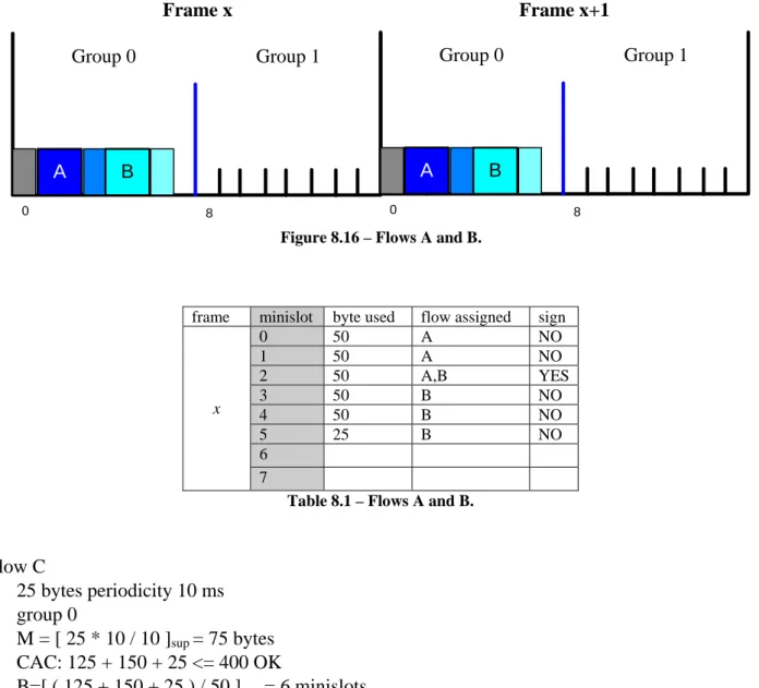
M = [ 250 * ( 10 / 30 ) ]sup = 84 bytes B = [ 84 / 50 ]sup = 2 minislots 0 8 Group 0 Group 1 A 0 8 Group 0 Group 1 A Frame x Frame x+1
Figure 8.14 – Flow allocation.
In order to reduce the MAC overhead, the allocations in the same group are combined together. This way, at most one physical preamble needs be sent for each group, and the amount of bytes
padded due to the OFDM symbol boundaries decreases.
Example
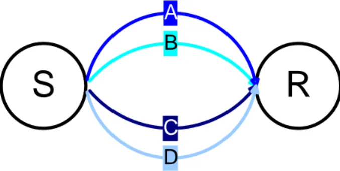
• 1 frame = 10 ms • 16 minislots per frame • 1 minislot = 50 bytes • 2 groups:
Group 0: SÆR Group 1: RÆS • 400 bytes per group
S
R
B
C
A
D
Figure 8.15 – Example with four flows.
Flow A
• 250 bytes periodicity 20 ms • group 0
• M = [ 250 * 10 / 20 ]sup = 125 bytes
• B= [ 125 / 50 ]sup = 3 minislots
Sender asks, for flow A, 125 bytes to Receiver; S knows that uses only 125 bytes, but has to allocate 3 minislots. Flow B • 300 bytes periodicity 20 ms • group 0 • M = [ 300 * 10 / 20 ]sup = 150 bytes • CAC: 125 + 150 <= 400 OK • B = [ ( 125 + 150 ) / 50 ]sup = 6 minislots
0 8 Group 0 Group 1 A B 0 8 Group 0 Group 1 A B Frame x Frame x+1
Figure 8.16 – Flows A and B.
frame minislot byte used flow assigned sign
0 50 A NO 1 50 A NO 2 50 A,B YES 3 50 B NO 4 50 B NO 5 25 B NO 6 x 7
Table 8.1 – Flows A and B.
Flow C • 25 bytes periodicity 10 ms • group 0 • M = [ 25 * 10 / 10 ]sup = 75 bytes • CAC: 125 + 150 + 25 <= 400 OK • B=[ ( 125 + 150 + 25 ) / 50 ]sup = 6 minislots
S asks, for flow C, 75 bytes to R; R allocates 2 minislots because it knows that it has allocate 25 bytes for flow B that S doesn’t use; so S uses this minislot for flow B and C.
The nodes have to think, in addition, that the fragmentation use further bytes.
If flow B finishes, S and R knows this situation and doesn’t release common minislots.
0 8 Group 0 Group 1 A B C 0 8 Group 0 Group 1 A B C Frame x Frame x+1
frame minislot byte used flow assigned sign 0 50 A NO 1 50 A NO 2 50 A,B YES 3 50 B NO 4 50 B NO 5 50 B,C YES 6 50 C NO x 7
Table 8.2 – Flows A, B and C.
Flow D • 25 bytes periodicity 10 ms • group 0 • M = [ 25 * 10 / 10 ]sup = 25 bytes • CAC: 75 + 150 + 75 + 25 <= 400 OK • B = [ ( 125 + 150 + 75 + 25 ) / 50]sup = 8 minislots 0 8 Group 0 Group 1 A B C 0 8 Group 0 Group 1 A B C Frame x Frame x+1 D D
Figure 8.18 – Flows A, B, C and D.
frame minislot byte used flow assigned sign
0 50 A NO 1 50 A NO 2 50 A,B YES 3 50 B NO 4 50 B NO 5 50 B,C YES 6 50 C NO x 7 25 D NO
Table 8.3 – Flows A, B, C and D.
In the previous example, for simplicity, I have not include MAC header, CRC and fragmentation sub-header, but EBRP include the size of the MAC header and CRC (i.e. 12 bytes) and the fragmentation sub-header needed to split the MAC SDUs into multiple MAC PDUs (i.e. one byte). Finally, note that the slots allocated may not be all completely used by the traffic flows, due to the variations in the packet size and generation interval with respect to the nominal values advertised upon admission. However, this capacity can be re-used to transmit backlogged best-effort data, if any.