CHAPTER IV RESULTS 4.1. In vivo experiments

(1)

CHAPTER IV RESULTS

4.1. In vivo experiments

An adequate in-vivo experimentation is essential for the next-data elaboration, because even the best algorithm can not correct inappropriate stimuli application or electrode positioning derived problems.

A few issues have to be taken into account before the experimental procedure, for an optimal experimentation:

1. In order to check the electrode functionality, the impedance measurements have to be done at the start of every experiment; if the impedance is high it can indicate electrode’s failure or bad positioning (e.g. cuff is not any more around the nerve)

2. Electromagnetic noise is very acute problem (e.g. can change base-line, or the quantity of noise- giving the false results in feature extraction ), that can be reduced by using Faraday’s cage and correct grounding.

All recordings have been performed in classical tripolar configuration. In this mode we obtained 25 cuff ENG signals-ready to be processed.

These few advices can help very much in overcoming the basic problems in ENG recording-setup. All registrations have been performed in classical tripolar configuration.

(2)

4.2.Data elaboration

The data elaboration process applied can be divided in the following steps: 1. Spectral analysis

2. Pre-processing 3. Feature extraction 4. Feature reduction 5. Pattern recognition

All steps are explained better in the next sections..

4.2.1.Spectal analysis

The most important step in neural signal processing is unquestionably the filtering of the “raw” signal. In order to implement the most appropriate filtering the spectral analysis has been performed. Results of all classical spectral analysis instruments, as Discrete Fourier Transform (DFT), Short Time Fourier Transform (STFT), Power of Spectrum and Power Spectral Density (DSP) of raw (unfiltered) cuff signals, indicated that, for the particular electrode configuration used in these experiments, the most significant portion of neural signal energy lies in a narrow frequency band between 1.0–2.0 kHz, in accordance with [19].

The same analysis has been carried out in parallel for rest-noise signal and for Signal of Interest (SOI). The SOI was taken as the part of ENG signal corresponding to all stimuli applied, without noise part of the signal, while for noise part only non stimulation parts of signal was explored. In fig 4.1. the noise (rest) signal with corresponding DFT, STFT, PS, DSP is presented.

(3)

a

b)

(4)

d)

e)

Fig.4.1.Spectral analysis of rest(noise) signal:

a) Raw signal b)DFT of signal c)Power of spectrum d)STFT e)PSD

In the DFT and PS graphic the peak above 1.0 KHz can be observed, in accordance with [19]. The STFT graphic shows uniform intensity of frequency distribution and finally the graph of PSD is similar to white noise PSD graphic.

Afterwards the spectral analysis of SOI has been performed-by taking the parts of signal corresponding to six different states of stimulation, without rest state, as presented in Fig. 4.2.

(5)

a) b) c) 0 0.5 1 1.5 2 2.5 3 3.5 4 4.5 5 -0.4 -0.3 -0.2 -0.1 0 0.1 0.2 0.3 Time-seconds V o lt s

(6)

d)

e)

Fig.4.2.Spectral analysis of SOI: a)Raw signal b)DFT of signal c)Power of spectrum d)STFT e)PSD

As supposed, there are big differences with respect to the rest signal. DFT and PS indicates that the peak is shifted to higher frequencies, with bigger absolute value. The important energy component which can be observed below 300 Hz, that can be attributed to Electromyography (EMG) signals (muscular activity), produced during the stimulation of efferent activity by means of reflex response.

In STFT graph higher intensity colours can be observed corresponding to times of stimuli application, indicating higher frequencies context in moments of stimulation. A similar conclusion can be seen in the case of PSD.

(7)

4.2.2.Preprocessing

The spectral analysis, although giving an idea about spectral context of neural signal recorded, did not give an unambiguous solution for appropriate filtering: there is certain overlap between rest and SOI frequency context, moreover, EMG noise in low frequencies (see Fig.4.2.b)), as the thermal one in high frequencies, compromise SNR.

The raw signal recorded above 2.0 kHz is dominated by thermal noise [12] (from both the amplifier and electrode), whose power is proportional to the square-root of the bandwidth utilized.

Thus, an upper frequency cutoff limit can be derived by optimizing the trade-off between (possibly) obtaining additional nerve signal energy using a higher cutoff frequency, and a reduction of the filtered signal’s SNR due to the increased contribution of thermal noise in the high frequency band. Consistent with previous results [12], a neural signal peak between 1.0 and 2.0 kHz was observed. Therefore, the lower frequency filter cutoff point can be obtained by optimizing another trade-off: the rejection of interfering muscle (EMG) signal verses the incorporation of additional low-frequency nerve signal information. Although the EMG signal power falls off rapidly above 100 Hz, some measurable energy content may be present at frequencies as high as 1 kHz [15].

Basically three types of filtering has been implemented: 1. Band pass filtering (as recommended in [12] ) 2. High pass filtering (as recommended in [13])

3. Band pass filtering-resulting from our spectral analysis.

In order to choose the best filtering all data elaboration has been done with all of three filters, eventually choosing the filtering which gave the best classification results.

(8)

4.3. Magnitude response of filter corresponding to band pass filter with bandwidth of 1.6–1.9 kHz ( -3 dB).

In Fig. 4.3. magnitude response of band pass filter designated according to [12] is presented. It is FIR equiripple 132 order band pass filter with bandwidth of 1.6–1.9 kHz ( -3 dB), with stop-bands below 60 dB.

In the present study, although, this filter did not give good performance (the worst between three). Afterwards, as recommended in [13], the high pass filter with 1KHz cutoff frequency has been implemented. In Fig.4.4. its magnitude response is presented.

4.4. Magnitude response of filter corresponding to high pass filter, with cutoff of 950 Hz ( -3 dB) It is FIR equiripple 244 order high pass filter with cutoff of 950 Hz ( -3 dB), with stop-bands of 60 dB. This filtering permitted good classification rates, but still inferior to those of third and the best one.

(9)

a)

b)

Fig.4.5.Raw signal(a) and its DFT(b)

The DFT , in its intrinsic mathematical form provides two parallel portions of signal’s spectrum. Obviously, only the one collocated in lower frequencies has physical sense.(In this study there is already, during the recording analogical band-pass filtering between 10 Hz and 5KHz, hence the portion between 16 and 20KHz from the graphic above cannot exist). In Fig.4.6. the result of high pass filtering is presented.

(10)

a)

b)

Fig.4.6. Representation of high pass filtrated signal(a), and its corresponding DFT(b) Best results gave our own band pass filtering. In Fig. 4.7. is represented its magnitude response.

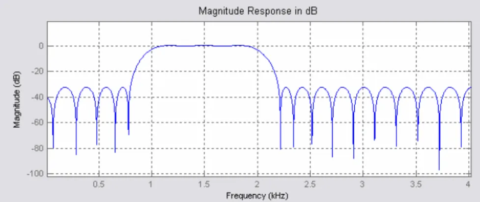
Fig. 4.7.Magnitude response of band pass filter with bandwidth of 1.0–2.0 kHz ( -3 dB)

It is FIR equiripple 101 order band-pass filter with bandwidth of 1.0–2.0 kHz ( -3 dB). . This filtering allowed for the best classification rates.

(11)

a)

b)

Fig.4.8. Band-pass filtered signal(1.0KHz-2KHz)(a) and its DFT(b)

This band pass filtering allowed the best classification to be obtained in our experimental study. The next step to perform proceeding with data elaboration is feature extraction.

(12)

4.2.3. Feature extraction

In pattern recognition, features are the individual measurable heuristic1 properties of the phenomena being observed. Choosing discriminating and independent features is key to any pattern recognition algorithm being successful in classification.

Features are usually numeric, but structural features such as strings and graphs are used in syntactic pattern recognition.

While different areas of pattern recognition obviously have different features, once the features are decided, they are classified by a much smaller set of algorithms. These include nearest neighbour classification in multiple dimensions, neural networks or statistical techniques such as Bayesian approaches[16].

In the present work different features, proposed in literature, have been extracted in order to find the most appropriate sub-set.

Here are presented the features which have been tested.

4.2.3.1. Time Domain Features

1. The rectified bin integration (RBI) is one of the most classic methods to extract features in EMG and ENG data elaboration.

In Fig 4.9. the filtered signal , ready for feature extraction step, with labels of stimulation times is presented. In Fig.4.10. the RBI, for a specific set of data, for different observation windows used during the elaboration is given.

1

A heuristic is a replicable method or approach for directing one's attention in learning, discovery, or problem-solving. It is originally derived from the Greek "heurisko" (εὑρίσκω), which means "I find". (A form of the same verb is found in Archimedes ' famous exclamation "eureka!" – "I have found [it]!") The term was introduced in the 4th century AD by Pappus of Alexandria.

(13)

0 20 40 60 80 100 120 -0.4 -0.2 0 0.2 0.4 0.6 0.8 1 Time[seconds] V o lt s

Signal with labels(red)

a) 0 20 40 60 80 100 120 -1.5 -1 -0.5 0 0.5 1 Time[seconds] N o rm a liz z e d s ig n a l v a lu e

ENG signal with labels(red)

b) Fig.4.9. ENG signal with labels of stimulation times(real voltage scale)-(a); Normalized ENG signal

(14)

0 200 400 600 800 1000 1200 0 0.1 0.2 0.3 0.4 0.5 0.6 0.7 0.8 0.9 1

RBI 100msec observation window

a) 0 100 200 300 400 500 600 700 800 0 0.1 0.2 0.3 0.4 0.5 0.6 0.7 0.8 0.9 1

RBI on 150msec window

b) Fig.4.10. Normalized RBI for (a)100msec observation window (b) 150msec observation window.

(15)

2. The Mean absolute value (MAV), or often used, integral of absolute value IAV=N*MAV, is the amplitude based feature-very often used. Its form is presented in Fig.4.10.

0 200 400 600 800 1000 1200 0 0.1 0.2 0.3 0.4 0.5 0.6 0.7 0.8 0.9 1

MAV 100msec observation window

a) 0 100 200 300 400 500 600 700 800 0 0.1 0.2 0.3 0.4 0.5 0.6 0.7 0.8 0.9 1

MAV on 150msec window

b) Fig.4.11. Normalized MAV for (a)100msec observation window (b) 150msec observation window

(16)

4. The Wavelength (WL) gives in same time amplitude and frequency information. This feature is presented, for a specific set of data in Fig.4.11.

0 200 400 600 800 1000 1200 0 0.1 0.2 0.3 0.4 0.5 0.6 0.7 0.8 0.9 1

Wavelength 100msec observation window

a) 0 100 200 300 400 500 600 700 800 0 0.1 0.2 0.3 0.4 0.5 0.6 0.7 0.8 0.9 1

Wavelength on 150msec window

(17)

5. The first two AR coefficients (as proposed in [15]) have been extrapolated too. Although they did not give good classification performance. These features can be observed, for a specific set of data in Fig.4.12. 0 200 400 600 800 1000 1200 1 1.005 1.01 1.015 1.02 1.025

AR1 100msec observation window

a) 0 200 400 600 800 1000 1200 0.99 0.992 0.994 0.996 0.998 1 1.002

AR2 100msec observation window

b)

(18)

6. The Variance (Second order expectation) is a statistic feature, is a statistic feature, used as an index of dispersion. In our study it presented very good discriminating results. In Fig. 4.13. this feature, for a specific set of data, is given.

0 200 400 600 800 1000 1200 0 0.1 0.2 0.3 0.4 0.5 0.6 0.7 0.8 0.9 1

VAR 100msec observation window

a) 0 100 200 300 400 500 600 700 800 0 0.1 0.2 0.3 0.4 0.5 0.6 0.7 0.8 0.9 1

VAR on 150msec window

b) Fig.4.13. Normalized VAR for (a)100msec observation window b) 150msec observation window

(19)

7. The variance with 2 lag delay also gave very good results, especially in combination with VAR, and fourth order statistics. In Fig. 4.14. this feature, for a specific set of data, is presented.

0 200 400 600 800 1000 1200 -1 -0.9998 -0.9996 -0.9994 -0.9992 -0.999 -0.9988

VAR2 100msec observation window

a) 0 100 200 300 400 500 600 700 800 0 0.1 0.2 0.3 0.4 0.5 0.6 0.7 0.8 0.9 1

VAR2 on 150 msec window

b)

(20)

8. The third order cumulant is a feature proposed in some authors [12],[20],[17] for eliminating the white noise, but in the present study did not give a good performance. In Fig. 4.15. this feature, for a specific set of data, is presented.

0 200 400 600 800 1000 1200 0 0.1 0.2 0.3 0.4 0.5 0.6 0.7 0.8 0.9 1

Third order cumulant 100msec observation window

a) 0 100 200 300 400 500 600 700 800 0 0.1 0.2 0.3 0.4 0.5 0.6 0.7 0.8 0.9 1

Third order moment on 150 msec window

b)

Fig.4.15. Normalized third order cumulant for (a)100msec observation window (b) 150msec observation window

(21)

9. The fourth order cumulant is proposed in [12],[20],[17] as one good idea for eliminating the white noise, and here gave good performance in combination with two second order moments: VAR and 2lag delay VAR. In 4.16. this feature is presented for a specific data set.

0 200 400 600 800 1000 1200 0 0.1 0.2 0.3 0.4 0.5 0.6 0.7 0.8 0.9 1

Fourth order cumulant 100msec observation window

a) 0 100 200 300 400 500 600 700 800 0 0.1 0.2 0.3 0.4 0.5 0.6 0.7 0.8 0.9 1

Fourth order moment on 150 msec window

b)

Fig.4.16. Normalized fourth order cumulant for (a)100msec observation window b) 150msec observation window

(22)

4.2.3.2. Frequency Domain Features

The information in neural signals is transmitted in part by frequency modulation of impulses. With cuff electrodes it is possible to record the sumatory activity of all the fibers activated within a time -hence frequency information may be very useful. We tried three different frequency based features. 1. The DFT was extrapolated on windows of observation, hence giving the same response as STFT-where the frequency context is located in time. The DFT feature is presented in Fig. 4.17.

0 200 400 600 800 1000 1200 0 0.1 0.2 0.3 0.4 0.5 0.6 0.7 0.8 0.9 1

STFT 100msec observation window

a) 0 100 200 300 400 500 600 700 800 0 0.1 0.2 0.3 0.4 0.5 0.6 0.7 0.8 0.9 1 STFT on 150msec window b)

(23)

2. Wavelet denoising was extrapolated with Symleth7 of fifth level decomposition with a soft threshold as in [13]. Because of the empirical nature of soft threshold in this method it is not automatic, and we have not found it informative. This feature, for a specific data set, can be seen in Fig.4.17. 0 200 400 600 800 1000 1200 0 0.1 0.2 0.3 0.4 0.5 0.6 0.7 0.8 0.9 1

Wavelets 100msec observation window

(24)

3.The Power Spectral Density(PSD) is one time-frequency representation. In our study it gave good performance, and was almost always indicated as most informative with PCA. Fig.4.18.shows this feature. 0 200 400 600 800 1000 1200 0 0.1 0.2 0.3 0.4 0.5 0.6 0.7 0.8 0.9 1

PSD 100msec observation window

a) 0 100 200 300 400 500 600 700 800 0 0.1 0.2 0.3 0.4 0.5 0.6 0.7 0.8 0.9 1 PSD on 150 msec window b)

(25)

4.2.4. Feature reduction

All above described features have been tested in plenty of signals in order to find the optimal sub-set which would give:

1. The best classification results

2. Acceptable number of features for real time calculation

This is the critical point of all the loop. Mathematics and computer science provide some instruments which can help in resolving this task, as PCA, Feed-Forward Selection, or ICA. In this study the first one has been implemented, but, as shown in of the following results, it has not given good classification results.

The PCA is based on the strong (and many times correct) assumption that the signal information is contained in its dispersion (variance), and it fails in many real cases. The first example that justifies the assumption is the case of residual artefacts (which can remain even after filtering), which will give a large variance without informational context. The most clear case is by looking the features above where AR has not information context but has quite high variance.

In this study many reduction sets have been tried in parallel, and finally the tests remaining are: In this study many reduction sets have been tried in parallel, and finally the tests remaining are:

1. Two first PCA set 2. MAV

3. VAR

4. MAV+VAR

(26)

4.2.5. Pattern recognition

Pattern recognition is a sub-topic of machine learning. It can be defined as "the act of taking in raw data and taking an action based on the category of the data". Pattern recognition aims at classifying data (patterns) based on either a priori knowledge or on statistical information extracted from the patterns. The patterns to be classified are usually groups of measurements or observations, defining points in an appropriate multidimensional space. This in contrast to pattern matching, where the pattern is rigidly specified.

A complete pattern recognition system consists of a sensor that gathers the observations to be classified or described; a feature extraction mechanism that computes numeric or symbolic information from the observations; and a classification or description scheme that does the actual job of classifying or describing observations, relying on the extracted features.

The classification or description scheme is usually based on the availability of a set of patterns that have already been classified or described. This set of patterns is termed the training set and the resulting learning strategy is characterized as supervised learning. Learning can also be unsupervised, in the sense that the system is not given an a priori labeling of patterns, instead it establishes the classes itself based on the statistical regularities of the patterns.

The classification or description scheme usually uses one of the following approaches: statistical (or decision theoretic), syntactic (or structural). Statistical pattern recognition is based on statistical characterisations of patterns, assuming that the patterns are generated by a probabilistic system. Syntactical (or structural) pattern recognition is based on the structural interrelationships of features. A wide range of algorithms can be applied for pattern recognition, from very simple Bayesian classifiers to much more powerful neural networks.

In our case, we have a-priori information of the system (labels of stimuli) and are using them to train our classifiers.

(27)

In the final tests four classifiers were used in parallel (see the previous Chapter for their description) :

1. Linear Discriminate Classifier (Bayesian) 2. Parzen’s classifier

3. KNN classifier 4. ANN classifier

In next section the performance of the four different classifiers are given. They have been obtained by using three different windows of observation, and in parallel with five different feature sets.

4.2.5.1. Classification results

In order to understand the limits of single-channel cuff electrodes to discriminate afferent signals the classifiers have been used to identify the stimuli grouped in different ways (two, three, four at a time or all the five stimuli). This approach allowed us also to verify whether the results achieved can be considered in accordance with the neurophysiology of the PNS.

Complete list of classifiers results can be see in last section of this chapter; while our goal was to find the limit possibilities-the best achievable classification results, which are presented in next section.

(28)

4.2.5.2.Best classification representation

The pattern recognition was performed with different subsets of six different stimuli. Here are presented in order.

4.2.5.3.Two stimuli Von Frey and Proprioceptive

a) b) 0 20 40 60 80 100 120 140 160 0 0.5 1 1.5 2 2.5 3 3.5 4

States predicted(red) respect real states(blu) of stimulation

0 1 2 3 4 5 6 7 8 9 10 x 105 -1 -0.8 -0.6 -0.4 -0.2 0 0.2 0.4 0.6 0.8 1

(29)

c)

d)

Fig.4.19. a)ENG signal with labels of VF and Proprioceptive stimuli; b) Classification results-red predicted state, blue-real state c) Best classification with corresponding feature sets d) Confusion

matrix for highest classification case Von Frey versus Nocioceptive

a)

Observation window 50 msec 100 msec 150 msec

Correct classification 82.17% 85.65% 89.54%

Classifier& feature set

ANN-IAV+VAR2 ANN-Hos ANN-IAV+VAR2

Diagonal-Correct hits Predicted rest Predicted VF Predicted Proprio

77 1 0 7 29 3 4 1 31 0 1 2 3 4 5 6 7 8 9 10 x 105 -1 -0.8 -0.6 -0.4 -0.2 0 0.2 0.4 0.6 0.8 1

(30)

b) c) Diagonal-Correct hits Predicted rest Predicted VF Predicted Nocio 75 1 5 6 27 9 9 3 27 d)

Fig.4.19. a)ENG signal with labels of VF and Nocioceptive stimuli; b) Classification results-red predicted state, blue-real state c) Best classification with corresponding feature sets d) Confusion

matrix for highest classification case

ANN-Hos ANN-Hos ANN-Hos

0 20 40 60 80 100 120 140 160 180 0 0.5 1 1.5 2 2.5 3 3.5 4 4.5 5

(31)

Proprioceptive versus Nocioceptive

a)

b)

Observation window 50 msec 100 msec 150 msec

Correct classification 73.61% 80.48% 81.24%

Classifier& feature set

KNN-VAR2 ANN-HOS ANN-HOS

c) 0 50 100 150 200 250 300 0 0.5 1 1.5 2 2.5 3 3.5 4 4.5 5

0 2 4 6 8 10 12 x 105 -1 -0.8 -0.6 -0.4 -0.2 0 0.2 0.4 0.6 0.8 1

(32)

Diagonal-Correct hits Predicted rest Predicted VF Predicted Nocio 75 1 5 6 27 9 9 3 27 d)

Fig.4.20. a)ENG signal with labels of Propriosepive and Nocioceptive stimuli; b) Classification results-red predicted state, blue-real state c) Best classification with corresponding feature sets d)

Confusion matrix for highest classification case Scratch versus Von Frey

a) b) 0 20 40 60 80 100 120 140 160 180 0 0.5 1 1.5 2 2.5 3

0 1 2 3 4 5 6 7 x 105 -0.8 -0.6 -0.4 -0.2 0 0.2 0.4 0.6 0.8 1

(33)

Observation window 50 msec 100 msec 150 msec Correct classification 81.60% 83.92% 82.14%

ANN-VAR2 ANN-VAR2 KNN-IAV+VAR2

c) Diagonal-Correct hits Predicted rest Predicted Scratch Predicted VF 90 10 0 0 7 0 11 6 44 d)

Fig.4.21. a)ENG signal with labels of Propriosepive and Nocioceptive stimuli; b) Classification results-red predicted state, blue-real state c) Best classification with corresponding feature sets d)

Confusion matrix for highest classification case Proprioceptivo versus Efferente

a) 0 1 2 3 4 5 6 7 8 9 10 x 105 -1 -0.8 -0.6 -0.4 -0.2 0 0.2 0.4 0.6 0.8 1

(34)

b)

Observation window 50 msec 100 msec 150 msec Correct classification 71.43% 71,00% 71.43%

ANN-IAV+VAR2 LDC-HOS ANN-IAV+VAR2 c)

Diagonal-Correct hits

Predicted rest Predicted Proprio Predicted Efferente 56 1 19 8 30 1 15 0 24 d)

Fig.4.22. a)ENG signal with labels of Propriosepive and Efferente stimuli; b) Classification results-red presults-redicted state, blue-real state c) Best classification with corresponding feature sets d)

Confusion matrix for highest classification case

0 20 40 60 80 100 120 140 160 0 1 2 3 4 5 6

(35)

Brush versus Scratch a) b) 0 20 40 60 80 100 120 0 0.2 0.4 0.6 0.8 1 1.2 1.4 1.6 1.8 2

0 0.5 1 1.5 2 2.5 3 3.5 4 4.5 5 x 105 -0.8 -0.6 -0.4 -0.2 0 0.2 0.4 0.6 0.8 1

(36)

Correct classification 69.18% 66,10% 65.89%

KNN-HOS KNN-HOS KNN-HOS

c)

Diagonal-Correct hits Predicted rest Predicted Brush Predicted Scratch

64 4 0

16 8 1

14 5 6

d)

Fig.4.22. a)ENG signal with labels of Brush and Scratch stimuli; b) Classification results-red predicted state, blue-real state c) Best classification with corresponding feature sets d) Confusion

matrix for highest classification case 4.2.5.4. Three stimuli VF, Proprioceptive, Nocioceptive a) 0 5 10 15 x 105 -1 -0.8 -0.6 -0.4 -0.2 0 0.2 0.4 0.6 0.8 1

(37)

b)

ANN-HOS KNN-2PCA KNN-HOS

Rest VF Proprio Nocio

122 5 3 9

2 25 1 3

1 3 28 2

9 1 1 27

d)

Fig.4.23. a)ENG signal with labels of VF, Proprioceptive, Nocioceptive stimuli; b) Classification results-red predicted state, blue-real state c) Best classification with corresponding feature sets d)

Confusion matrix for highest classification case

0 50 100 150 200 250 0 0.5 1 1.5 2 2.5 3 3.5 4 4.5 5

(38)

Scratch ,VF, Proprioceptive

a)

b) Observation

window

50 msec 100 msec 150 msec

Correct classification

79.65% 81.88% 84.82%

ANN-2PCA ANN-2PCA ANN-HOS

c) 0 20 40 60 80 100 120 140 160 180 200 0 0.5 1 1.5 2 2.5 3 3.5 4

0 2 4 6 8 10 12 x 105 -1 -0.8 -0.6 -0.4 -0.2 0 0.2 0.4 0.6 0.8 1

(39)

Rest VF Proprio Efferent 101 10 2 2 0 5 1 0 5 2 27 2 4 0 1 29 d)

Fig.4.24. a)ENG signal with labels of Scratch, VF and Proprioceptive stimuli; b) Classification results-red predicted state, blue-real state c) Best classification with corresponding feature sets d)

Brush, Scratch, VF a) 0 1 2 3 4 5 6 7 8 9 10 x 105 -0.8 -0.6 -0.4 -0.2 0 0.2 0.4 0.6 0.8 1

(40)

b)

Correct classification 74.35% 74.35% 74.50%

KNN-2PCA KNN-2PCA ANN-VAR2+IAV

c) Rest Brush predicted Scratch predicted VF predicted 80 7 6 2 2 2 3 3 3 1 7 1 5 5 1 25 d)

Fig.4.25. a)ENG signal with labels of Brush, Scratch, VF stimuli; b) Classification results-red predicted state, blue-real state c) Best classification with corresponding feature sets d) Confusion

0 20 40 60 80 100 120 140 160 0 0.5 1 1.5 2 2.5 3

(41)

VF, Nocioceptive, Efferent

a)

b)

Observation window 50 msec 100 msec 150 msec

Correct classification 65.62% 70.41% 74.90%

KNN-HOS ANN-HOS ANN-HOS

c) 0 50 100 150 200 250 0 1 2 3 4 5 6

0 5 10 15 x 105 -1 -0.8 -0.6 -0.4 -0.2 0 0.2 0.4 0.6 0.8 1

(42)

Rest VF Nocio Efferent 100 2 4 23 6 26 2 0 11 3 35 0 10 0 0 21 d)

Fig.4.26. a)ENG signal with labels of VF, Nocioceptive, Efferentstimuli; b) Classification results-red predicted state, blue-real state c) Best classification with corresponding feature sets d) Confusion

Proprioceptive, Nocioceptive, Efferent

a) 0 5 10 15 x 105 -1 -0.8 -0.6 -0.4 -0.2 0 0.2 0.4 0.6 0.8 1

(43)

b) Observation

window

50 msec 100 msec 150 msec Correct

classification

63.44% 66.93% 71.66%

KNN-HOS ANN-HOS ANN-HOS c) Rest Proprio Predicted Nocio predicted Efferent predicted 104 1 10 22 7 28 4 0 14 3 25 1 6 0 2 20 d)

Fig.4.27. a)ENG signal with labels of Proprioceptive, Nocioceptive, Efferent stimuli; b) Classification results-red predicted state, blue-real state c) Best classification with corresponding feature sets d)

0 50 100 150 200 250 0 1 2 3 4 5 6

(44)

4.2.5.5. Four stimuli

VF,Proprioceptive, Nocioceptive, Efferent

a) b) 0 50 100 150 200 250 300 350 0 1 2 3 4 5 6

0 0.2 0.4 0.6 0.8 1 1.2 1.4 1.6 1.8 2 x 106 -1 -0.8 -0.6 -0.4 -0.2 0 0.2 0.4 0.6 0.8 1

(45)

Observation window

50 msec 100 msec 150 msec

Correct classification

65.90% 70.81% 75.16%

KNN-HOS HOS ANN-IAV+VAR2 c)

Rest Scratch VF Proprio Nocio

148 2 0 12 24 5 27 4 2 0 4 1 29 2 0 12 1 1 21 2 7 0 0 1 17 d)

Fig.4.28. a)ENG signal with VF,Proprioceptive, Nocioceptive, Efferent labels of stimuli; b) Classification results-red predicted state, blue-real state c) Best classification with corresponding

feature sets d) Confusion matrix for highest classification case Scratch,VF,Proprioceptive, Nocioceptive a) 0 2 4 6 8 10 12 14 16 18 x 105 -1 -0.8 -0.6 -0.4 -0.2 0 0.2 0.4 0.6 0.8 1

(46)

b)

Correct classification 71.50% 75% 75%

KNN-HOS KNN-HOS KNN-HOS

c)

Rest Scratch VF Proprio Nocio

202 10 6 11 22 8 8 0 2 0 10 4 33 8 6 7 0 2 27 5 17 1 3 2 26 d)

Fig.4.29. a)ENG signal with labels of Scratch, VF, Proprioceptive, Nocioceptive stimuli; b) Classification results-red predicted state, blue-real state c) Best classification with

corresponding feature sets d) Confusion matrix for highest classification case

0 50 100 150 200 250 300 0 0.5 1 1.5 2 2.5 3 3.5 4 4.5 5

(47)

Brush, Scratch, VF, Efferent a) b) 0 50 100 150 200 250 300 350 0 1 2 3 4 5 6

0 5 10 15 x 105 -0.8 -0.6 -0.4 -0.2 0 0.2 0.4 0.6 0.8 1

(48)

Observation window

63.48% 66.57% 66.09%

KNN-HOS ANN-HOS ANN-HOS c)

Rest Brush Scratch VF Efferent

149 18 16 6 26 0 1 2 0 0 2 0 4 1 0 7 6 3 40 0 30 0 0 0 39 d)

Fig.4.30. a)ENG signal with labels of Brush, Scratch, VF, Efferent stimuli; b) Classification results-red presults-redicted state, blue-real state c) Best classification with corresponding feature sets d)

Confusion matrix for highest classification case 4.2.5.6. Five stimuli

Scratch,VF,Propriosepitve, Nocioceptive, Efferent

a) 0 0.5 1 1.5 2 2.5 x 106 -1 -0.8 -0.6 -0.4 -0.2 0 0.2 0.4 0.6 0.8 1

(49)

b)

Correct classification

64.05% 70.24% 67.72%

KNN-HOS ANN-HOS ANN-2PCA

c)

Rest Scratch VF Proprio Nocio Efferent

254 11 1 0 24 36 0 4 0 1 0 0 12 6 37 7 6 0 8 2 3 38 5 0 11 0 3 4 23 4 16 0 0 0 1 24 d)

Fig.4.30. a)ENG signal with labels of Scratch, VF, Proprioceptive ,Nociosetive ,Efferent stimuli b) Classification results-red predicted state, blue-real state c) Best classification with

corresponding feature sets d) Confusion matrix for highest classification case

0 100 200 300 400 500 600 0 1 2 3 4 5 6

(50)

Brush, Scratch,VF, Proprioceptive, Nocioceptive a) b) 0 50 100 150 200 250 300 350 400 450 500 0 0.5 1 1.5 2 2.5 3 3.5 4 4.5 5

0 0.2 0.4 0.6 0.8 1 1.2 1.4 1.6 1.8 2 x 106 -1 -0.8 -0.6 -0.4 -0.2 0 0.2 0.4 0.6 0.8 1

(51)

Observation window

50 msec 100 msec 150 msec Correct classification 69.74% 72.61% 73.21% Classifier& feature set ANN-HOS ANN-HOS ANN- 2PCA-same as HOS c)

Rest Brush Scratch VF Proprio Nocio

161 7 6 3 9 13 0 0 1 0 0 0 2 2 9 3 0 0 5 6 1 22 1 0 4 0 0 1 20 3 14 0 0 2 3 23 d)

Fig.4.31. a)ENG signal with labels of Brush, Scratch, VF, Proprioceptive ,Nocioceptive stimuli b) Classification results-red predicted state, blue-real state c) Best classification with

corresponding feature sets d) Confusion matrix for highest classification case 4.2.5.7. All(six) stimuli a) 0 0.5 1 1.5 2 2.5 x 106 -1 -0.8 -0.6 -0.4 -0.2 0 0.2 0.4 0.6 0.8 1

(52)

b) Observation

window

63.57% 66.28 67.88%

Classifier & feature set

ANN-HOS KNN-HOS ANN-HOS

c)

Rest Brush Scratch VF Proprio Nocio Efferent

186 10 10 5 1 12 27 0 0 0 0 0 0 0 1 1 4 0 0 0 0 3 4 3 23 2 0 0 4 0 0 0 28 5 0 17 0 0 3 2 22 5 11 0 0 0 0 0 12 d)

Fig.4.32. a)ENG signal with labels of all stimuli b)Classification results-red predicted state, blue-real state c) Best classification with corresponding feature sets d) Confusion matrix for highest

classification case 0 50 100 150 200 250 300 350 400 450 0 1 2 3 4 5 6

(53)

4.2.5.8. Complete tables of classification results

In next tables section are represented performances of four different classifiers, obtained for three different windows of observation, and in parallel with five different feature sets. For all tables is valid the same legend(on the end of section).

Two stimuli

2.1. PROPIOSEPTION_VF

2.2. VF_NOCIOSEPTION

50 msec 100 msec

LDC PAR KNN ANN LDC PAR KNN ANN 2PCA 71.08 76.08 76.95 76.73 74.34 79.56 79.13 72.17 MAV 73.26 77.17 78.04 78.26 76.92 78.26 81.73 73.69 VAR 72.17 78.91 78.69 77.86 73.47 82.60 80.43 80.43 MAV+VAR 73.69 77.17 78.04 82.17 76.08 80.43 81.72 83.47 HOS 76.30 76.87 77.32 81.52 80.86 77.82 81.74 85.65 150 msec LDC PAR KNN ANN 2PCA 76.47 86.92 83.00 81.69 MAV 78.43 86.27 85.62 86.27 VAR 80.39 86.92 86.92 87.58 MAV +VAR 80.39 86.27 85.62 89.54 HOS 82.35 84.31 84.96 80.39 50 msec 100 msec

LDC PAR KNN ANN LDC PAR KNN ANN 2PCA 62.65 64.62 63.94 65.43 67.21 65.48 63.52 66.39 MAV 60.13 62.57 60.79 61.55 64.34 65.90 65.57 65.98 VAR 65.49 67.68 69.73 69.32 61.88 71.72 69.67 71.72 MAV+VAR 69.52 63.19 60.73 73.20 75.81 65.98 65.57 81.56 HOS 73.61 65.43 62.57 75.86 79.09 65.16 63.44 79.91 150 msec LDC PAR KNN ANN 2PCA 72.22 70.37 72.22 71.61 MAV 69.75 64.19 61.72 67.28 VAR 69.75 77.77 66.04 67.28 MAV +VAR 78.39 64.10 61.28 79.62 HOS 81.48 70.37 65.43 81.48

(54)

2.3. BRUSH_SCRATCH

2.4. EFFERENT_PROPIOSEPTION

50 msec 100 msec

(55)

2.5. PROPIOSEPTION_NOCIOSEPTION

2.6. VF_SCRATCH

50 msec 100 msec

LDC PAR KNN ANN LDC PAR KNN ANN 2PCA 75.66 79.22 79.22 79.52 80.35. 82.73 82.73 83.33 MAV 74.48 81.00 81.00 80.77 80.95 83.92 83.92 83.92 VAR 72.10 81.60 81.30 81.60 76.78 82.73 82.14 83.33 MAV+VAR 77.44 81.00 81.01 81.00 82.73 83.92 83.92 83.92 HOS 73.88 79.22 78.63 80.31 77.97 83.14 83.14 83.33 150 msec LDC PAR KNN ANN 2PCA 75.89 81.25 78.57 57.14 MAV 75.89 81.25 82.14 79.46 VAR 74.10 82.14 81.25 78.57 MAV +VAR 79.46 81.25 82.14 76.78 HOS 76.78 83.03 78.57 80.45

(56)

Three stimuli 3.1. VF_PROPIOSEPTION_NOCIOSEPTION

3.2. VF_NOCIOCEPTIVE_EFFERENT

50 msec 100 msec

(57)

3.3. SCRATCH_VF_PROPRIOCEPTIVE

3.4. PROPRIOCEPTIVE_NOCIOCEPTIVE_EFFERENT

50 msec 100 msec

(58)

3.5. VF_BRUSH_SCRATCH

Four stimuli

4.1. VR_PROPIOSEPTION_NOCIOSEPTION_SCRATCH

50 msec 100 msec

(59)

4.2. VR_PROPIOSEPTION_NOCIOSEPTION_EFFERENT

4.3. BRUSH_SCRATCH_VF_EFFERENT

50 msec 100 msec

(60)

Five stimuli 5.1. VR_PROPIOSEPTION_NOCIOSEPTION_EFFERENT

5.2. BRUSH_SCRATCH_VF_PROPIOSEPTION_NOCIOSEPTION

50 msec 100 msec

(61)

All(six) stimuli

6. BRUSH_SCRATCH_VF_PROPIOSEPTION_NOCIOSEPTION_EFFERENT

Tables legend:

2PCA: The first two principal components MAV: Mean absolute value

VAR: Variance

HOS: Higher order statistics – VAR + 2 lag delay VAR + fourth order moment LDC: Linear discriminate classifier (Bayesian)

PAR: Parzen classifier

KNN: K-nearest neighbor classifier ANN: Artificial Neural Network classifier

50 msec 100 msec