Alma Mater Studiorum
· Universit`a di Bologna
Scuola di Scienze
Dipartimento di Fisica e Astronomia Corso di Laurea Magistrale in Fisica
Science of complex systems and
future-sca↵olding skills: a pilot study with
secondary school students
ALLEGATI
Relatore:
Prof.ssa Olivia Levrini
Correlatori:
Dott.ssa Giulia Tasquier
Dott.ssa Laura Branchetti
Presentata da:
Eleonora Barelli
Index of the annexes
!Annex A1 - Non-linearity of complex systems: the Lotka-Volterra model (complete
version) ... 2
Annex A2 - Non linearity of complex systems: the Lotka-Volterra model (tutorial version) ... 11
Annex A3 - Non-linearity of complex systems and sensitivity to initial conditions: the logistic map ... 20
Annex A4 – Questionnaire on the concept of feedback ... 31
Annex A5 - Self-organization in complex systems: the world of ants ... 34
Annex A6 - Synthesis of the fifth IPCC report: the global warming issue ... 36
Annex A7 - Map of global warming ... 40
Annex A8 - Use and Production of Bio Fuels: the “Biodiesel story” ... 41
Annex A9 - Cause-effect map of the “Biodiesel story” ... 46
Annex A10 - Feedback loops for the “Biodiesel story” ... 47
Annex A11 - Cause-effect map of the “Biodiesel story” with the feedback areas highlighted ... 48
Annex A12 - The Fishback Game: rules of the game ... 49
Annex A13 - The Fishback Game: printable material ... 51
Annex A14 - The Fishback Game: feedback loops ... 57
Annex A15 - Probable, possible and desirable futures for the Town Irene ... 58
Annex A16 - Pre-questionnaire (Q1) ... 66
Annex A17 - Intermediate questionnaire (Q2) ... 69
Annex A18 - Introduction to Logical Framework Approach ... 71
Annexes
Annex A1 - Non-linearity of complex systems: the
Lotka-Volterra model (complete version)
!
The Lotka–Volterra equations, also known as the predator–prey equations, are a pair of first order, non-linear, differential equations frequently used to describe the dynamics of biological systems in which two species interact, one as a predator and the other as prey. Two variables have to be considered: the number of preys (x) and that of predators (y). Both the populations change through time, so we refer to x(t) as the number of preys at time t and to y(t) as the number of predators at the same time. So, the equations can be written in this way:
!
Now we are explaining in some details the components of these equations, for a better understanding about the characteristics of the model.
! and respectively indicate the variation of the population of preys and predators over time: they are called growth rates.
A, B, C and D are positive coefficients used to detail the interaction between the species: -! A is the coefficient of birth of preys; the bigger is A, the faster is the positive
contribution to the growth rate of preys.
-! B is the coefficient of predation; it indicates how fast the predators eat preys and, multiplied for both the number of preys and predators, it negatively contributes to the growth rate: indeed, the bigger is B, the faster x decreases.
-! C is the coefficient of encounter between preys and predators; multiplied for x and y, C represents the growth of the predator population. It could seem similar to the coefficient of predation B but a different constant is used because the rate at which the predator population grows is not necessarily equal to the rate at which it consumes the prey.
-! D is the coefficient of natural death of predators; multiplied for the number of predators themselves, it negatively contributes to the growth rate: indeed, the bigger is D, the faster y decreases.
The zero-interaction model
If there was not any significant interaction between the two species, we would have to set B = C = 0, and in this way just A and D would remain. The two equations become:
! !
This simplified version of the equations allows us to better understand the assumptions of the model. In absence of predators, the first equation is a typical differential equation which gives as a solution the exponential function:
!
where x0 is the number of preys at time t. The same happens for y(t), with the only
difference that the solution is a negative exponential: ! where y0 is the number of predators at time t.
Hence, we can highlight some assumptions of the Volterra-Lotka model:
-! the prey population finds ample food at all times and, in absence of predators, grows indefinitely, since the preys do not die by natural death (Assumption 1); -! in absence of preys to eat, the predators population decreases by natural death,
since its food supply depends entirely on the size of the prey population (Assumption 2).
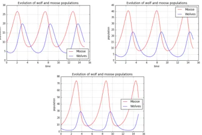
A simulation written in Python programming language can be easily used to prove the behaviour of the model, plotting the evolutions of the moose and wolf populations. For example, with a suitable choice of parameters1 and initial conditions, the resulting plot is shown in Figure 1. The exponential behaviour of both the time evolutions – positive for the preys and negative for the predators – is evident.
!
Figure 1. Exponential evolution of preys (moose) and predators (wolves) with this choice of parameters A = 0.1, B = 0.00001, C = 0.00001, D = 0.5
and initial conditions x0 = 50, y0 = 100.
!!!!!!!!!!!!!!!!!!!!!!!!!!!!!!!!!!!!!!!!!!!!!!!!!!!!!!!!
1!It is not possible to set B = C = 0 because the calculus of the equilibrium position would
be impossible for the programme (division by 0 is not defined). So, one has to choose B and C so that the relation !holds.!
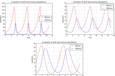
The periodic solutions of the model
Now, we can go back to the initial formulation of the complete equations of the model and, resetting the parameters at “normal” values (without B and C being near 0), the output of the programme is the periodic plot in Figure 2.
Figure 2. Periodic evolution of preys (moose) and predators (wolves) with this choice of parameters A = 1, B = 0.1, C = 0.075, D = 1.5 and initial
conditions x0 = 10, y0 = 5.
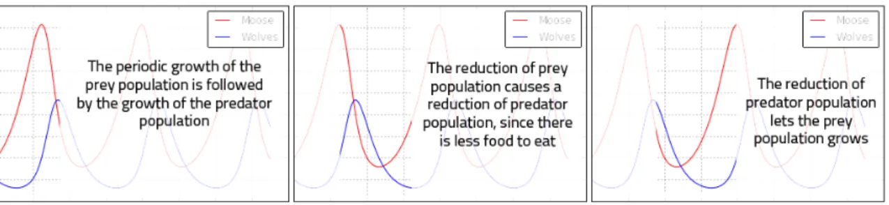
For every running of the algorithm, the plot displays the periodic solutions of our system of equations, given the parameters and the initial conditions that we chose. These oscillations can be explained identifying in Figure 2 the subsequent phases of increasing and decreasing of populations. This procedure is reported in three steps in Figure 3.
Figure 3. Comments about the periodic evolution of preys (moose) and predators (wolves), with respect to their time evolution in Figure 2.
If we stop at this stage of the analysis, we remain within a linear conception of causality: one step calls a second one which causes another one. But we could imagine to continue the reasoning begun in Figure 3 in order to see explicitly the positive feedback loop that is the cause of the time oscillation of this system. This procedure is displayed in Figure 4.
Figure 4. Reinterpretation of the linear explanation in Figure 3 as a circular positive feedback loop.
Discovering the meaning of the parameters
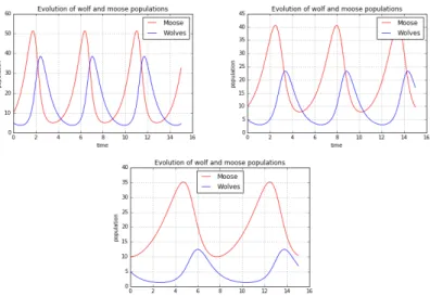
Changing the values of the parameters of the model, their meaning and role can be better understood. It is convenient to change only one parameter at each running of the script, so that its role can be separated from that of the other ones. In Figure 5, 6, 7 and 8 we respectively let A, B, C and D change; the initial conditions are set at x0 = 10 and y0 = 5.
The parameter A controls the birth rate of preys. In Figure 5, from left to right, A decreases and the time required for the growth of the moose population grows. In a certain sense, A controls the period of the time oscillation.
Figure 5. Dependence of the time evolution from the parameter A: 5.left) A = 1.5, B = 0.1, C = 0.075, D = 1.5, 5.centre) A = 1, B = 0.1, C = 0.075, D
= 1.5, 5.right) A = 0,5, B = 0. 1, C = 0.075, D = 1.5.
The parameter B indicates how frequently the preys are eaten by the predators. In Figure 6, from left to right, B decreases; he period of the oscillations remains the same but, when
B gets smaller, the maximum value of predator population sensitively changes (blue curves are lower and lower). This is reasonable because, if the predation is very frequent, the number of predators grows up to high values, while, at the opposite, if the predation is a rare fact, the predators cannot reach an high number of samples.
Figure 6. Dependence of the time evolution from the parameter 6: 4.left) A = 1, B = 0.04, C = 0.075, D = 1.5, 6.centre) A = 1, B = 0.1, C = 0.075, D =
1.5, 6.right) A = 1, B = 0.2, C = 0.075, D = 1.5.
The parameter C is the coefficient of encounter between preys and predators. About it, the same comments made above with regard to B hold true.
Figure 7. Dependence of the time evolution from the parameter C: 7.left) A = 1, B = 0.1, C = 0.1, D = 1.5, 7.centre) A = 1, B = 0.1, C = 0.075, D =
1.5, 7.right) A = 1, B = 0.1, C = 0.05, D = 1.5.
The parameter D is the coefficient of natural death of predators. An high value of D means that the predators die frequently, allowing preys to grow more rapidly and to reach higher values of individuals. As D decreases, the period of oscillation changes as well as the maximum number of preys and predators.
Figure 8. Dependence of the time evolution from the parameter D: 8.left) A = 1, B = 0.1, C = 0.075, D = 4, 8.centre) A = 1, B = 0.1, C = 0.075, D =
1.5, 8.right) A = 1, B = 0.1, C = 0.075, D = 0.75. From the model to the reality
After having discovered the meaning and role of all the parameters of the model and its interpretation at the light of circular causality, the results of our simulation can be compared with real data. We can consider a famous example of the predator-prey relationship: the one between wolves and moose on Isle Royale, an island in Lake Superior in Michigan. This unique relationship has been subject of detailed study for over 55 years because it is considered very similar to the situation described from the model. Indeed, being an isolated island, there is little migration of animals into and out of it and, as a national park, human interaction and impact on the two species is also limited.
The applet
http://www.phschool.com/atschool/phbio/active_art/predator_prey_simulation/! shows the ideal behaviour of the model (obtained with a programme like the one we used above) versus the real data measured for wolves and moose on Isle Royal. The experimental curves are reported in Figure 9.
Figure 9. 40 years evolution of the wolf and moose population on Isle Royale.
The graph obtained in Figure 9 is very different to the periodic evolution showed in all the plots above. This requires a comment about the other implicit assumptions of the model that we have not noticed yet: during the process described from the model, the environment does not change in favour of one species and there are not any factors (diseases, famines, genetic mutations, fitness problems…) that cause premature deaths or damages for the one or both the populations (Assumption 3). This is not the case of Isle Royale’s interaction.
As an isolated island, the Isle Royale initially had neither wolves nor moose. The moose are believed to have either swam across Lake Superior from Minnesota in the early 1900s; in 1949 a pair of wolves crossed an ice bridge from Ontario to the island during a harsh winter. But because only one pair or wolves migrated to the island, they have suffered from severe inbreeding, losing genetic variability (all the wolves’ DNA on Isle Royale can be traced back to one ancestor). Inbreeding leads to mutations and fitness problems, often accompanied by violent social rejection by other wolves. So, the Assumption 3 does not hold true.
Moreover, moose prefer birch and aspen trees, which used to grow plentifully on the island, but over a century of moose browsing have been largely replaced by the less nutritious balsam fir. But also the resources of balsam fir are limited: it is observed that when the moose population grows too high, the balsam fir population crashes, leading to a crash in the moose population. This is a negative feedback loop and it makes the Assumption 1 not verified.
Also the Assumption 2 is not true for the Isle Royale case. Indeed, moose make up nine-tenths of a wolf’s diet: the remaining 10% consists of snowshoe hares and beavers. So, there are not only two species in interaction and the Lotka-Volterra model cannot be reasonably applied.
Possible improvements of the model… and a sad conclusion
The model can be improved by adding parameters which take into account some elements that help in order to make the model more similar to the real situation. With the applet already mentioned, it is possible to set a value also for two other coefficients:
-! habitat variability: how often factors other than the ones you are controlling, such as density-independent factors (weather), and density-dependent factors (disease) change. This parameter has value between 1, if the habitat is not so variable, and 100, if it is extremely variable;
-! carrying capacity: the largest number of individuals of a population that a given environment can support. This parameter is an average percentage and it is included between 50% and 150%.
Changing their values it is possible to see the changes in the graphs with respect to the standard Lotka-Volterra. Anyway it can be easily recognized that, like all the models, through all the possible improvements with the addition of other coefficients, it can never take into account the whole complexity of the real world. Using other words: also the use of the two parameters described, that had the main goal of relaxing the validity conditions
of the model, is not enough to reproduce the experimental behaviour for moose and wolves on Isle Royale.
About the Python script: structure and comments
In the followings, we report the brief Python script for the integration of Lotka-Volterra equations, adding comments about the structure and the role of the functions used. In red are written the lines of code that have to be modified by the user in order to obtain the different plots described above.
Firstly, from the library numpy the operation of multiplication is imported, an abbreviation for the library pylab is chosen and the four parameters of the model are defined at default values.
from numpy import * import pylab as p
a = 1 b = 0.2 c = 0.075 d = 1.5
Now we have to define the function named dX_dt, which has X and t (set equal to 0 by default) as its arguments; this function returns an array of two components: the first component is the right side member of the preys equation, while the second component is the right side member of the predators equation. The notation X[0] indicates the first component of the vector X[1], while X[1] refers to its second component.
def dX_dt(X, t=0):
return array([ a*X[0] - b*X[0]*X[1] , c*X[0]*X[1] - d*X[1]])
After having defined the parameters and the function to be integrated, we need to import from the library scipy the function integrate, written to integrate a system of ordinary differential equations. The 1000 components vector t is defined: its first component is 0, its last one is 15 and linspace automatically add other 998 equispaced components. X0 is the 2-dimensional vector in which we set the initial conditions for the prey population (first component) and the predator one (second component). Now, it is possible to use the function integrate: the first argument is the function dX_dt that we want to integrate, the second one is the vector of initial conditions and the third one is a sequence of time points for which to solve for our function.
from scipy import integrate t = linspace(0, 15, 1000)
X0 = array([10, 5])
X = integrate.odeint(dX_dt, X0, t)
Finally we use Matplotlib to plot the evolution of both populations and save the figure obtained in the same folder in which is the script file (note that if you subsequently run the script, the file is overwritten at each launch).
moose, wolves = X.T f1 = p.figure()
p.plot(t, moose, 'r-', label='Moose') p.plot(t, wolves , 'b-', label='Wolves') p.grid()
p.legend(loc='best') p.xlabel('time')
p.ylabel('population')
p.title('Evolution of wolf and moose populations') f1.savefig('moose_and_wolves_1.png')
! !
Annex A2 - Non linearity of complex systems: the
Lotka-Volterra model (tutorial version)
!
The Lotka–Volterra equations, also known as the predator–prey equations, are a pair of first order, non linear, differential equations frequently used to describe the dynamics of biological systems in which two species interact, one as a predator and the other as prey. Two variables have to be considered: the number of preys (x) and that of predators (y). Both the populations change through time, so we refer to x(t) as the number of preys at time t and to y(t) as the number of predators at the same time. So, the equations can be written in this way:
!
Now we are explaining in some details the components of these equations, for a better understanding about the characteristics of the model.
! and respectively indicate the variation of the population of preys and predators over time: they are called growth rates.
A, B, C and D are positive coefficients used to detail the interaction between the species: -! A is the coefficient of birth of preys; the bigger is A, the faster is the positive
contribution to the growth rate of preys.
-! B is the coefficient of predation; it indicates how fast the predators eat preys and, multiplied for both the number of preys and predators, it negatively contributes to the growth rate: indeed, the bigger is B, the faster x decreases.
-! C is the coefficient of encounter between preys and predators; multiplied for x and y, C represents the growth of the predator population. It could seem similar to the coefficient of predation B but a different constant is used because the rate at which the predator population grows is not necessarily equal to the rate at which it consumes the prey.
-! D is the coefficient of natural death of predators; multiplied for the number of predators themselves, it negatively contributes to the growth rate: indeed, the bigger is D, the faster y decreases.
The zero-interaction model
If there was not any significant interaction between the two species, we would have to set B = C = 0, and in this way just A and D would remain. Write the new form of the equations with this choice of parameters:
! !
! ! ! ! ! !
This simplified version of the equations allows us to better understand the assumptions of the model. In absence of predators, the first equation is a typical differential equation which gives as a solution the exponential function:
!
where x0 is the number of preys at time t. The same happens for y(t), with the only
difference that the solution is a negative exponential: ! where y0 is the number of predators at time t.
Hence, we can highlight some assumptions of the Volterra-Lotka model:
-! the prey population finds ample food at all times and, in absence of predators, grows indefinitely, since the preys do not die by natural death (Assumption 1); -! in absence of preys to eat, the predators population decreases by natural death,
since its food supply depends entirely on the size of the prey population (Assumption 2).
A simulation written in Python programming language can be easily used to prove the behaviour of the model, plotting the evolutions of the moose and wolf populations. The parts of the codex that you need to modify during the following exercises are those related to the value of parameters A, B, C and D and to the initial conditions x0 and y0:
# Definition of parameters: default a= 1, b=0.1, c=0.075, d=1.5 a = 1
b = 0.2 c = 0.075 d = 1.5
X0 = array([10, 5]) # initials conditions: 10 moose and 5 wolves
Make a choice of parameters for reproducing a zero-interaction model. Note that it is not possible to set B = C = 0 because the calculus of the equilibrium position would be impossible for the programme (division by 0 is not defined). So, one has to choose B and
C so that this relation holds:!
Draw the time evolution displayed by the simulation, writing also the values of parameters and initial conditions that you have set.
! ! ! ! ! ! !
The exponential behaviour of both the time evolutions – positive for the preys and negative for the predators – should be evident.
The periodic solutions of the model
Now, we can go back to the initial formulation of the complete equations of the model and, resetting the parameters at default values, draw the resulting plot reporting the parameters and the initial conditions that you have fixed.
! ! ! ! ! ! ! !
For every running of the algorithm, the plot displays the periodic solutions of our system of equations. Try to explain these oscillations (increasing and decreasing of populations) adding a comment for each graph.
If we stop at this stage of the analysis, we remain within a linear conception of causality: one step calls a second one which causes another one. But we could imagine to continue the reasoning: add arrows that connect the steps above… now you can see explicitly the positive feedback loop that is the cause of the time oscillation of this system.
Discovering the meaning of the parameters
Changing the values of the parameters of the model, their meaning and role can be better understood. It is convenient to change only one parameter at each running of the script, so that its role can be separated from that of the other ones. Let A, B, C and D change, setting the initial conditions fixed at default value (x0 = 10 and y0 = 5).
Draw three plots obtained with changed values of A (take care of the scales on the population axis!). For each plot, report the values of A that you used for your simulation. ! ! ! ! ! ! ! ! !
The parameter A controls the birth rate of preys. Look at your plots: what happens if A decreases? So, what you can think could be the meaning of this parameter?
! !
! !
Draw three plots obtained with changed values of B. For each plot, report the values of B that you used for your simulation.
! ! ! ! ! ! ! ! !
The parameter B indicates how frequently the preys are eaten by the predators. Look at your plots: what happens if B decreases? So, what you can think could be the meaning of this parameter? ! ! ! ! ! !
Draw three plots obtained with changed values of C. For each plot, report the values of C that you used for your simulation.
! ! ! ! ! ! ! ! ! ! ! !
The parameter C is the coefficient of encounter between preys and predators. Look at your plots: what happens if C decreases? Why is it so similar to the behaviour we obtain changing B?
!
! ! !
Draw three plots obtained with changed values of D. For each plot, report the values of D that you used for your simulation.
! ! ! ! ! ! ! ! ! ! ! !
The parameter C is the coefficient of natural death of predators. Look at your plots: what happens if D decreases? ! ! ! ! ! ! From the model to the reality
After having discovered the meaning and role of all the parameters of the model and its interpretation at the light of circular causality, the results of our simulation can be compared with real data. We can consider a famous example of the predator-prey relationship: the one between wolves and moose on Isle Royale, an island in Lake Superior in Michigan. This unique relationship has been subject of detailed study for over 55 years because it is considered very similar to the situation described from the model. Indeed, being an isolated island, there is little migration of animals into and out of it and, as a national park, human interaction and impact on the two species is also limited.
The applet
http://www.phschool.com/atschool/phbio/active_art/predator_prey_simulation/! shows the ideal behaviour of the model (obtained with a programme like the one we used above) versus the real data measured for wolves and moose on Isle Royal.
What are the graphical similarities and what are the differences between the ideal plots that you obtained before and this graph of real data?
! ! ! ! ! !
These differences requires a comment about the other implicit assumptions of the model that we have not noticed yet: during the process described from the model, the environment does not change in favour of one species and there are not any factors (diseases, famines, genetic mutations, fitness problems…) that cause premature deaths or damages for the one or both the populations (Assumption 3). This is not the case of Isle Royale’s interaction.
As an isolated island, the Isle Royale initially had neither wolves nor moose. The moose are believed to have either swam across Lake Superior from Minnesota in the early 1900s; in 1949 a pair of wolves crossed an ice bridge from Ontario to the island during a harsh winter. But because only one pair or wolves migrated to the island, they have suffered from severe inbreeding, losing genetic variability (all the wolves’ DNA on Isle Royale can be traced back to one ancestor). Inbreeding leads to mutations and fitness problems, often accompanied by violent social rejection by other wolves. So, what of our 3 assumptions does not hold true?
Assumption number __
Moreover, moose prefer birch and aspen trees, which used to grow plentifully on the island, but over a century of moose browsing have been largely replaced by the less nutritious balsam fir. But also the resources of balsam fir are limited: it is observed that when the moose population grows too high, the balsam fir population crashes, leading to a crash in the moose population. This is a negative feedback loop and it makes an other of the assumptions not verified. What?
Assumption number __
Also another assumption is not true for the Isle Royale case. Indeed, moose make up nine-tenths of a wolf’s diet: the remaining 10% consists of snowshoe hares and beavers. So, there are not only two species in interaction and the Lotka-Volterra model cannot be reasonably applied. What of our 3 assumptions does not hold true?
Possible improvements of the model… and a sad conclusion
The model can be improved by adding parameters which take into account some elements that help in order to make the model more similar to the real situation. With the applet already mentioned, it is possible to set a value also for two other coefficients:
-! habitat variability: how often factors other than the ones you are controlling, such as density-independent factors (weather), and density-dependent factors (disease) change. This parameter has value between 1, if the habitat is not so variable, and 100, if it is extremely variable;
-! carrying capacity: the largest number of individuals of a population that a given environment can support. This parameter is an average percentage and it is included between 50% and 150%.
Changing their values it is possible to see the changes in the graphs with respect to the standard Lotka-Volterra. Anyway you can easily recognized that, also with these new parameters, it is impossible to fit the experimental data. What do you think is the cause of this impossibility? ! ! ! ! ! ! ! !
Annex A3 - Non-linearity of complex systems and sensitivity to
initial conditions: the logistic map
!
The logistic map was introduced in 1976 as a discrete-time demographic model analogous to the logistic equation. The logistic equation has the following form:
and it is a first-order non-linear differential equation. The non linearity is given from the fact that the derivative does not depend only on f(x) but there is also a quadratic term f2(x).
The discretization of the logistic equation leads to the logistic map:
where xn is a number in the interval [0, 1] that represents the ratio of existing population
to the maximum possible population (also called carrying capacity of the environment) and r is a positive parameter (we do not want negative populations).
It is an iterative map because it establishes the value of a variable at time n+1, by knowing the value at time n and the evolution rule. There are many ways of interpreting it: a possible way is looking at it as a curve in the plane (in this case the parabolic function can be recognized) but a second way is as a series of instructions:
-! give some number xn, subtract its square xn2 and multiply the result for the constant
r;
-! call the result xn+1;
-! given xn+1 do nothing but call it xn;
-! repeat the first step with the value found in step 3.
The first three instruction together form a mapping of one number on to another:
and the addition of the fourth step results in an iterated mapping. We can use the symbol mn(xn) to represent the nth iterate of the original value xn. The instructions require to
generate a series of number, called orbit:
xn, m(xn), m2(xn), m3(xn), … , mn(xn), …
The initial value xn is called the seed of the orbit.
The demographic logistic model
The simple logistic equation written above is a formula for approximating the evolution of an animal population over time. We can write again the formula distinguishing into brackets the two terms of the product.
We are going to comment the two terms separately.
-! rxn: since not every existing animal will reproduce (a portion of them are male),
not every female will be fertile, not every conception will be successful, and not every pregnancy will be successfully carried to term, the population increase will be some fraction of the present population. The term of proportionality r is the growth rate or fecundity and approximates the rate of successful reproduction. Limiting the model at this term, it produces exponential growth without limit. -! (1 - xn): since every population is bound by the physical limitations of its territory,
some allowance must be made to restrict this growth. If there is a carrying capacity of the environment, then the population may not exceed that capacity, otherwise the population would become extinct. This can be modelled by multiplying the population by a number that approaches zero as the population approaches its limit. If we normalize xn to this capacity, the multiplier (1 − xn) has the role
explained.
Playing with the parameter r
By varying the parameter r several kinds of behaviour are observed. If the growth rate expressed by r is set too low, the population will die out and go extinct: in Figure 1 this behaviour is shown, because r is in the interval [0, 1].
Figure 1. Extinction of the population within the 10th generation for r = 0.5. Higher growth rates might settle the population toward a stable value represented by : in Figure 2 we observe this evolution, because r is chosen in the interval [1, 2].
Figure 2. Stabilisation of the population toward the value xn = 0.33, when r
= 1.5.
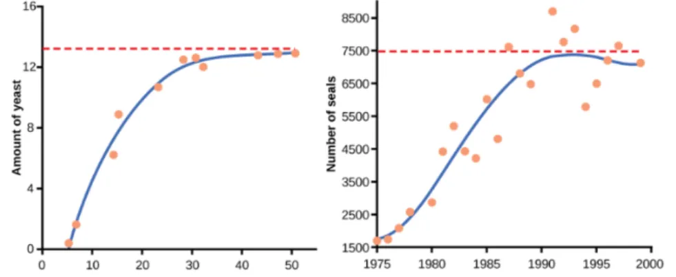
We can give two examples of this behaviour. Yeast, a microscopic fungus used to make bread and alcoholic beverages, exhibits a curve similar to that in Figure 2, when grown in a test tube (see Figure 2A.left). Its growth levels off as the population depletes the nutrients that are necessary for its growth.
In the real world, however, there are variations to this idealized curve. An example in wild populations is that of harbour seals (see Figure 2A.right). The population size exceeds the carrying capacity for short periods of time and then falls below the carrying capacity afterwards.
Figure 2A. Fitting ecological data with logistic model. 2A.left: yeast grown in ideal conditions in a test tube show a classical logistic growth curve (cfr.
Figure 2). 2A.right: a natural population of seals shows real-world fluctuation.
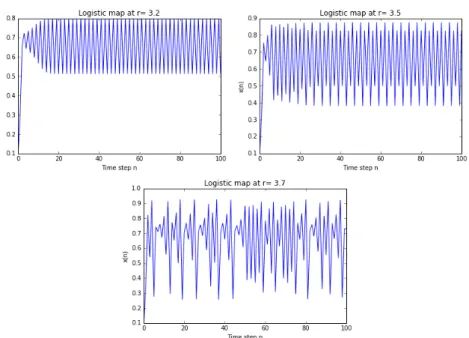
Another possible behaviour is the fluctuation across a series of population booms and busts. In Figure 3 we observe three different kinds of evolutions:
-! with r in [3, 1+ !3.44949] the population approaches permanent oscillations between two values dependent on r. We can think at this system as a switch that can stay on two states and the transition time between these two states is regular and dependent on r itself;
-! with r in [1+ , 3.56995] the population approaches periodic oscillations among 2k values. The system is now a multi-value switch, with a sequence of possible states that repeat following always the same order;
-! with r in [3.56995, 4] there are almost no more oscillations of finite period2: the value 3.56995 is often defined as the onset of chaos.
Figure 3. Fluctuation of the population across a series of booms and busts. 3.left: oscillation between two values, for r = 3.2. 3.centre: oscillation among 4 values, for r = 3.5. 3.right: chaotic behaviour without oscillations
of finite period, for r = 3.7. Limit cycles and strange attractors
After having showed some graphs for some values of the parameter r, it is useful to define a term and explain a concept often used in the study of complex system. An attractor is the value, or the set of values, that the system settles toward over time. For example, when r is set to 0.5 (see Figure 1), the system has a fixed-point attractor at population level 0: in other words, the population value is drawn toward 0 over time as the model iterates. Another example is shown when r is set to 3.5 (see Figure 3.centre): the system oscillates between four values. In both these cases the attractors are called limit cycles.
Passing the onset of chaos, the attractor is no more a limit cycle because chaotic systems have so called strange attractors, around which the system oscillates forever, never repeating itself or settling into a steady state of behaviour (see Figure 3.right). For a better understanding of this fact, let us see the so called bifurcation diagram, showed in Figure 4, obtained running the logistic model again across 1000 values of r in the interval [0, 4]. To read this kind of diagram, it is convenient to watch at it as 1000 discrete vertical slices, each one corresponding to one of the 1000 parameters between 0 and 4. For each one of
!!!!!!!!!!!!!!!!!!!!!!!!!!!!!!!!!!!!!!!!!!!!!!!!!!!!!!!!
2 Although most values of r beyond 3.56995 exhibit chaotic behaviour, there are still
these slices, the model has been run 450 times, then the first 200 values have been ignored3, so the final 250 generations for each growth rate remain.
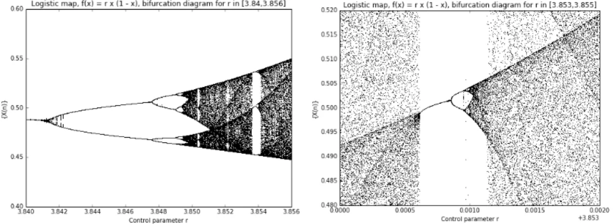
Figure 4. Bifurcation diagram for r in [0, 4].
Thus, each vertical slice depicts the population values that the logistic map settles toward for that parameter value. In other words, according to the definition given before, the vertical slice above each growth rate is that growth rate’s attractor. We can reinterpret the analysis and the comments done before about the role of the parameter r at the light of this new representation:
-! for r in [0, 1] the system always collapses to zero;
-! for r in [1, 3] the system always settles into an exact, stable population level; -! for r in [3, 1+ !3.44949] the system displays an oscillation between two
values;
-! for r in [1+ , 3.56995] the oscillation is between 4, 8, 16, 32 values (as it can be seen in Figure 5, where a zooming into the interval [2.95, 3.6] is provided);
Figure 5. Bifurcation diagram for r in [2.95, 3.6]: the progressive bifurcation in 2k values is observed; from this behaviour the diagram has
taken its name. !!!!!!!!!!!!!!!!!!!!!!!!!!!!!!!!!!!!!!!!!!!!!!!!!!!!!!!!
3!The first 200 values are ignored in order to avoid considering the transient phase that
does not define the attractor. For example, looking at Figure 1, if also the first six generations were considered, in the bifurcation diagram we would obtain a straight vertical segment for values of r in [0, 1], but these values would not be significant with respect to the stable evolution of the system that shows up beyond the transient phase. With this cut of the first iterations, we see, in the bifurcation diagram, just the attractor value 0, when r is in [0, 1].!
-! for r in [3.56995, 4] the diagram shows 250 different values, so a different value for each of its 250 generations: it means that the evolution never settles into a fixed point or a limit cycle. In Figure 6 a zoom on an interval in this area is provided.
Figure 6. Bifurcation diagram for r in [3.7, 3.9]: for almost each r, there are as many different possible values of population as the number of
generations. Fractals
The bifurcation diagram allows us to see another important property of many complex systems: the fractal structure. In the figures above can be recognized some particular patterns that exist at every scale, no matter how much we zoom into it: this properties is called self-similarity. Starting from Figure 6, we progressively zoom in the diagram: we can recognize the same bifurcation structure shown in figures above. A part of the process of zooming in is shown in Figure 7.
!
Figure 7. Zooming of bifurcation diagram: the fractal structure can be recognized.
Sensitivity at initial conditions and deterministic chaos
Another characteristic of the logistic model and of many other complex systems is the so called sensitivity at initial conditions. If we focus on the interval [3.56995, 4], we can
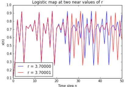
look at the time series from two different, but very close, initial conditions. For example, we can use r = 3.7, comparing it with another value that is only 10-5 away from the first one. The graph in Figure 8 is obtained: we can observe that it takes only two dozen iterates before the two curves diverge far away from each other.
Figure 8. Behaviour of the logistic map for two near values of r.
This chaotic behaviour and this difference between the two plots are due to the non linearity of the system and to the iterative structure of the map. Indeed, recalling the formula for the map, the quadratic term causes a quadratic sensitivity to errors about initial conditions; moreover, the iterative structure implies that an initial error spreads on the whole evolution of the system. That is why, despite its deterministic simplicity, over time this chaotic system produces totally unpredictable and wildly divergent behaviour. The plots seem to evolve randomly but there is a fundamental distinction between chaos and randomness: the logistic model continues to follow the very simple deterministic rule we have expressed at the beginning of our analysis, but produces an apparent randomness given by the aperiodicity. This phenomenon is called deterministic chaos and was discovered by Edward Lorenz who described chaos as “when the present determines the future, but the approximate present does not approximately determine the future.” This aspect is strictly linked to the mathematical modelling of complex systems and changes the meaning of knowledge and prediction about systems. Looking at the Figure 8, we can say that if our knowledge of those two systems started at generation 40, we would have no way of guessing that they were almost identical in the beginning. With chaos, history is lost to time and prediction of the future is only as accurate as the measurements. In real-world chaotic systems, measurements of initial conditions are never infinitely precise, so errors always compound, and the future becomes entirely unknowable given long enough time horizons.
This is famously known as the butterfly effect, from the title of a conference held by Lorenz in 1972. “Does the flap of a butterfly’s wings in Brazil set off a tornado in Texas?”. Now, we can answer: yes, it does. Small events compound and irreversibly alter the future of the universe.
Chaos can be observed in many physical systems, also outside the ecological context. For example, in mechanics, a system as simple as a double pendulum (see Figure 9) is a chaotic system because infinitesimal differences in the starting conditions lead to drastically different results as the system evolves.
Figure 9. Schematization of a double pendulum, that consists of a pendulum with another pendulum attached to its end.
If we plot the evolution in time of the angle "1 of the main arm and the angle "2 of the
second arm, changing the initial speeds of the main arm, the behaviour in Figure 10 is observed.
Figure 10. Time evolution of "1 (10.top) and "2 (10.bottom) for near initial
conditions. The red line refers to a double pendulum with v1 = 400.0 deg/s,
the blue line to a an identical pendulum with v1 = 400.1 deg/s.
For a short while the two pendulums stay in phase, but their behaviour quickly diverges even though their initial speeds are very similar (only 0.1 deg/sec difference in the initial speed of the main arm). This shows that the systems are sensitive to their initial conditions.
Perhaps not as obviously as this physical system has, particular electrical circuits also exhibit chaotic behaviour, starting from non-linear mathematical descriptions. Two examples are the varicap diode circuit and the Chua circuit.
Python scripts
Three Python scripts have been written in order to draw the plots reported in this work. In the followings the codes are reported with some comments; in red are written the lines of code that have to be modified by the user in order to obtain the different plots described above.
Logistic Map.py
The first script (LogisticMap.py) defines the logistic map and produces the plots from Figure 1 to Figure 3.
After having imported the plotting routines, simulations parameters are set. Particularly, a value for r is assigned, an array that will contain the value of population x is created
and initialized in its first component, and the number of iterations N is fixed.
from pylab import *
r = 3.7
x = [0.1]
N = 100
With a for loop, for N times the value xn+1 is calculated and appended to the list x. Finally,
the plot is drawn.
for n in range(0,N): x.append( r*x[n]*(1.-x[n]) ) xlabel('Time step n') ylabel('x(n)') title('Logistic map at r= ' + str(r)) plot(x , 'b') show() LogisticMap2NearInitialConditions.py
The second script (LogisticMap2NearInitialConditions.py) is similar to the first one but in this case two plots are drawn in a unique graph, because we want to control the sensitivity of the model to near values of the parameter r, in order to make graphs like that in Figure 8.
After having imported the plotting routine and set the parameter, initialized the array of population values and chosen the number of iteration, it is set the value of a constant named delta which represents the increment with respect to x1; an array x2 is also initialized.
from pylab import *
r = 3.7
x1 = [0.1]
delta = 1e-5
x2 = [x1[0] + delta]
With a for loop, for N times the values xn+1 are calculated and appended to the lists x1
and x2. Finally, the plots are drawn within a unique figure.
for n in range(0,N):
x1.append( r*x1[n]*(1.-x1[n]) ) x2.append( r*x2[n]*(1.-x2[n]) ) xlabel('Time step n')
ylabel('x(n)')
title('Logistic map at two near values of r') plot(x1, 'b', label="r = 3.70000")
plot(x2 , 'r', label="r = 3.70001") legend(loc='best')
show()
LogisticBifn.py
The third script (LogisticBifn.py) draws the bifurcation diagrams from Figure 4 to Figure 7.
The script begins with the importation of the modules needed.
from numpy import * from pylab import *
The logistic map’s function is defined and the parameter range is set up.
def LogisticMap(r,x):
return r * x * (1.0 - x)
rlow = 3.7 rhigh = 3.9
The plot is prepared.
figure(1,(8,6))
TitleString = 'Logistic map, f(x) = r x (1 - x), '
TitleString += 'bifurcation diagram for r in [%g,%g]' % (rlow,rhigh)
title(TitleString)
xlabel('Control parameter r') ylabel('{X(n)}')
To avoid the autoscaling that would be implicit in the plot function, we put dots at the corners of the desired data window.
plot([rhigh], [1.0], 'k,') plot([rhigh], [0.0], 'k,') plot([rlow], [0.0], 'k,') plot([rlow], [1.0], 'k,')
The value of initial condition x0 is set as ic; then, the number of transient generations is
set (these values will be thrown away). The parameter nIterates sets how much the attractor is filled in, while nSteps sets how dense the bifurcation diagram will be. The variable rInc represents the increment for the following calculations.
ic = 0.2
nTransients = 200 nIterates = 250 nSteps =1000
rInc = (rhigh-rlow)/float(nSteps)
With a for cycle (for exploring all the 1000 values of the parameter r) the initial
condition is set to the reference value, the transient iterations are thrown array and the next batch of iterates is stored in the array x. The plot function draws the list of (r, x) pairs as pixels. for r in arange(rlow,rhigh,rInc): state = ic for i in range(nTransients): state = LogisticMap(r,state) rsweep = [ ] x = [ ] for i in range(nIterates): state = LogisticMap(r,state) rsweep.append(r) x.append( state ) plot(rsweep, x, 'k,') show() References
Boeing, G. (2016). “Visual Analysis of Nonlinear Dynamical Systems: Chaos, Fractals, Self-Similarity and the Limits of Prediction.” Systems, 4 (4), 37.
http://csc.ucdavis.edu/~chaos/courses/nlp/Software/partE.html https://en.wikipedia.org/wiki/Logistic_map http://hypertextbook.com/chaos/ https://www.boundless.com/biology/textbooks/boundless-biology-textbook/population- and-community-ecology-45/environmental-limits-to-population-growth-251/logistic-population-growth-930-12186/! ! http://www.met.rdg.ac.uk/~ross/Documents/SchoolTalkDP.html
Annex A4 – Questionnaire on the concept of feedback
!
The questionnaire is based on the Ted-Ed video lesson
http://ed.ted.com/lessons/feedback-loops-how-nature-gets-its-rhythms-anje-margriet-neutel#watch
Which of the following is an example of a positive feedback loop?
A.! As glaciers melt, there is less white surface to reflect heat, which causes more melting
B.! As plants grow, their litter creates more soil humus, which in turn makes it hospitable for more plants
C.! "Violence breeds more violence” – or, a violent act by one group causes their enemy to retaliate with more violence
D.! All of the above
Negative feedback is called negative because ________. A.! It counteracts disturbance
B.! It causes degradation of an (eco)system C.! It has a destabilizing effect
D.! It has no effect on system stability
The strength of a feedback loop is ________.
A.! The sum of the positive link strengths in the loop B.! The sum of all the link strengths in the loop C.! The product of all the link strengths in the loop
D.! The sum of the positive link strengths divided by the sum of the negative link strengths in the loop
If you have a feedback loop with three strong negative links, and one of those links turns into a very weak positive link, what will the resulting feedback be?
A.! Strong positive feedback B.! Strong negative feedback C.! Weak positive feedback D.! Weak negative feedback E.! No feedback
How many feedback loops are possible in a food web of 20 species? A.! Up to 20
B.! Around 80 C.! Hundreds
D.! Thousands
How do all the feedbacks together in an ecosystem create harmony? One important mechanism is:
A.! The feedbacks become synchronized
B.! Positive feedbacks counteract destabilizing negative feedbacks
C.! Many populations interacting causes break-up of the chains of the short feedback loops
D.! Destabilising positive feedbacks are counteracted by negative feedbacks
The process of erosion on a landscape is an example of positive feedback. Can you describe a feedback loop that explains this process in more detail, starting with the feedback between plant, humus, and at least one more node in the network? Hint: you will have to add more than one negative link.
! ! ! ! ! ! !
Describe three examples of positive feedback and three of negative feedback, in other systems that have many interacting parts – such as economic, social, political systems.
! ! ! ! ! ! !
! ! ! ! ! ! ! ! ! ! ! ! !
One of the more prevalent feedback loops discussed today is one in relation to melting polar ice caps due to climate change. Is this a positive or negative feedback loop? Explain your answer.
! ! ! ! ! ! !
Annex A5 - Self-organization in complex systems: the world of
ants
!
Ants have some of the most complex social organization in the animal kingdom, living in structured colonies with different kinds of members who perform specific roles. But although this may sound similar to some human societies, this organization of the system does not arise from any higher level decisions or urban plans, but emerges from very basic rules of interaction between its parts. This kind of organization is better called, because of its properties, self-organization.
Ants have no methods of intentional communication but individual ants interact each other through touch, sound and chemical signals. These stimuli accomplish many things from serving as an alarm to other ants if one is killed, to signalling when a queen is nearing the end of her reproductive life. But one of the most impressive collective capabilities of ant colony is to thoroughly and efficiently explore large areas without any predetermined plan. Most species of ants have little or no sense of sight and can only smell things in their vicinity. Combined with their lack of high level coordination, this would seem to make them terrible explorers but there is an amazingly simple way that ants maximize their searching efficiency: by changing their movement patterns based on individual interactions. When two ants meet, they sense each other by touching antennae; if there are many ants in a small area this will happen more often, causing them to respond by moving in more convoluted, random paths in order to search more thoroughly. But in larger area, with less ants, where such meetings happen less often, they can walk in straight lines to cover more ground. While exploring their environment in this way, an ant may come across any number of things, from threats or enemies, to alternate nesting sites.
One of the most impressive capability that some species of ants have is known as recruitment: when one of these ants happens to find food, it will return with it, marking its path with a chemical scent; other ants will then follow this pheromone trail, renewing it each time they manage to find food and return. Once the food in that spot is depleted, the ants stop marking their return: the scent dissipates and ants are no longer attracted to that path.
A computer simulation
A lot of computer simulations have been written in order to reproduce the behaviour of ants in response at the presence of obstacles, food, caves or elements of scare. The video at this link https://www.youtube.com/watch?v=G5wb4f5n6qQ&t=29s shows the mode of operation of one of these simulations and the result is the spatial organization of ants according to pattern that seem to contradict the chaotic nature of this complex system. Particularly interesting is the mechanism of recruitment as shown in the simulation. In Figure 1 there are some examples of patterns followed by ants to go from the food (with points) to the caves (black points), passing through obstacles (grey points).
Figure 1. The recruitment mechanism makes spatial patterns emerge.
These seemingly crude methods of search and retrieval are, indeed, so useful that they are applied in computer models to obtain optimal solutions from decentralized elements, working randomly and exchanging simple information. Understanding the basis of self-organization could lead to improvements in swarm robotics, large numbers of simple robots working together, as well as self-healing materials and other systems capable of organizing and fixing themselves. More broadly, identifying the rules that ants obey could help scientists understand how biologically complex systems emerge (for example, how groups of cells give rise to organs).
References
Inside the ant colony – TED lesson by Deborah M. Gordon
https://www.youtube.com/watch?v=vG-QZOTc5_Q
http://naturedocumentaries.org/5519/what-ants-teach-deborah-gordon-ted-talk-2014/
Annex A6 - Synthesis of the fifth IPCC report: the global
warming issue
!
Global warming, in climatology, indicates an increase in the average temperature of Earth's surface and recorded in different phases of the climatic history of the Earth. The expression is now almost always used with heating significance due to the anthropogenic (i.e. human) contribution, decisive in the heating phase of the last 100 years. The fifth report of the Intergovernmental Panel on Climate Change (IPCC) in 2014 estimated that the average global surface temperature has increased by 0.85 [0.65-1.06] °C in the period 1880-2012. Most of the phenomena that cause the rise in temperature since the mid-twentieth century are considered, within the IPCC report, anthropogenic. These phenomena are responsible for an increase of the natural phenomenon of the greenhouse effect. The natural greenhouse effect is part of the complex of thermal equilibrium adjustment mechanisms of a planet (or satellite) surrounded by an atmosphere, which, if it contains certain gases called greenhouse gases indeed, produces the overall effect of mitigating the temperature the global average surface of the planet, isolating partially by large swings in temperature or that would subject the planet in their absence. For giving an idea of the phenomena regarding the Earth, in the absence of greenhouse gases, by the equation of balance between in- and outgoing radiation is one which average surface temperature of the Earth would be of about -18 °C whereas, thanks to the presence of greenhouse gases, the actual value is about +14 °C, enabling life as we know it. The greenhouse effect is man-made increase in the natural greenhouse effect phenomenon due to the emission of greenhouse gases by human activities, including industry, agriculture, livestock, transport, power plants for civilian purposes. In particular industries, transport, energy production facilities and even tourism activities contribute to increasing emissions from fossil fuels such as methane and carbon dioxide (CO2) while agriculture and livestock, more and more intensive activities, date the growing food demand, contribute most to the emission of nitrous oxide and methane. Most production of methane is indeed due to the fermentation of typical livestock manure, also grew significantly, and the fermentation of crops to submergence (for example rice). To the list of greenhouse gases should be added the chlorofluorocarbons (CFC), the only man-made gas, mainly used in the production of spray cans. This type of cans, now banned from production in different countries, have been the subject of debate between eighty and two thousand years as they are considered responsible for the depletion of the ozone layer in the atmosphere.
In addition to global warming, the emission of CO2 into the atmosphere as a result of human activity has been determining also the phenomenon known as “acidification of the seas”. As they explain on “Climalteranti”, “For avoiding any doubts, the 'acidification' term does not mean that the sea water becomes acidic (i.e. that its pH becomes less than 7), instead it means that the pH decreases (by a few tenths) but remained above 8 that is basic or alkaline land: rather than 'acidification' should therefore strictly speaking use the term 'de-alkalization'”.
However, the acidification mechanism is broadly explained in this way: around a third of the CO2 emitted by human activities is absorbed by the water of the seas where it turns into carbonic acid according to the reaction CO2 + H2O → H2CO3. The carbonic acid in water has a low concentration and rapidly dissociates to form carbonate and bicarbonate ions and liberating H + ions. More CO2 is emitted into the atmosphere, the greater the concentration of H +, which is measured by the decrease in pH.
The reduction in global average pH over the last two centuries or so has been recently estimated that more than 0.1 on the logarithmic pH scale corresponds to an increase of about 30% of H + ions. Among the most well-known effects of acidification of the seas is the damage to coral reefs but the phenomenon affects all the seas, not only tropical ones. “And the organisms affected by acidification are just at the beginning of the marine food chain at the other end of which we are humans, not just the trendy sushi eaters but all people living from fishing and make it their main source of protein”
(http://www.climalteranti.it/2010/07/16/il-gemello-cattivo-del-surriscaldamento-globale/).
Returning to the phenomenon of global warming, the first "Statement" IPCC lists several effects attributable to it with high confidence: increased sea temperatures; the melting of the polar ice caps and mountain ranges; the increase of extreme events like heavy rainfall, increased tropical cyclones and heat waves.
As will be described later, all these phenomena contribute, in different ways, to modify the environmental scenarios, economic and social, leading to a total increase of risk2 on the territory, with consequent increase in the social vulnerability3 and migration of the small and large scale .
The main consequence of the increase in sea temperatures with implications on human life is a change in the composition of the fish fauna. For example, in the Mediterranean Sea there has for some years a species of tropical input (tropicalization Mediterranean), in many cases lessepsian or penetrated from the Red Sea through the Strait of Suez4; in the more northern basins like those Italians we are witnessing instead an increase of southern thermophilic species first found only on the North African coast (south Mediterranean). Especially in the eastern part of the Mediterranean these processes are having significant effects on the survival of native species, since that change ecosystems and the food chain.
A second consequence of global warming is the reduction of the ice in the polar caps, the permafrost5, ice on the mountain and frozen seas chains. Some implications of these phenomena that are well documented are the change of the territory in the areas concerned (including changes to the biological and agriculture network), as well as the increased risk of flooding due to the increase of the waters that flow along the rivers. The phenomenon of flooding of river basins has become in recent years a major problem in some areas of the world as well as in parts of Europe and in Italy. At this, in addition to melting ice, contributes significantly to the intensification of rainfall, other consequences of global warming also mentioned below.
Since the early 70s, the mass loss of glaciers and ice caps in Greenland and Antarctica and thermal expansion of the seas realize set of about 75% the rising of the global average sea level (high confidence). This phenomenon, together with the increase of the risk of heavy storms, can cause extensive damage on the architectural and building urban structures present on the coasts, in addition to ecological damage due to salt water intrusion in coastal aquifers, the intrusion of salt wedge estuaries, the loss or modification of the marine and coastal biodiversity. All these impacts have strong implications on
business activities conducted in the coastal areas, but also on the recreational, tourism and historical, artistic, and of all the agricultural practices carried out in the hinterland that receive irrigation drawn from sources that, intrusion, have brackish water.
As a final result of global warming is the intensification of the number and violence of extreme weather events (such as heavy rainfall, cyclones, floods, droughts, heat waves, etc.).
The intensification of the phenomenon of floods and tropical cyclones, as well as damage crops and infrastructure, increases the housing insecurity and determines both economic losses of private due to the same disaster is an increase in expenses to which public institutions have to opposite to remedy the disasters.
Finally, in this review of extreme events, it has been observed as heat waves and the lengthening of the dry spells lead to further pressure on already scarce water resources, increasing, especially in poor countries, problems of access to drinking water. This climatic phenomenon therefore has serious consequences in terms of public health, and damage to crops and thus decrease in food safety6, as well as in terms of land degradation, desertification and causing decrease in green space.
From all of the mentioned above you can well understand how the magnitude of climate change has increased in recent decades the risk of certain territories exposed to extreme events to affect the livability same in some areas even at high social vulnerability. Entire populations in some areas of the world are no (or insufficient) access to water, with the consequence of not being able to ensure the survival of their family, not being able to secure their income from agriculture or livestock (drought in the fields, die-off of farms), of not being able to have access to food. From this arises the increase of "environmental migration" and "eco-refugee problem". Even harsher climatic conditions do not push to migrate, these extreme events can still cause a deterioration of the health status of the population, resulting in increased social vulnerability.
As claimed by the IPCC, to address the problems of climate change requires action both in terms of mitigation (action aimed at developing research and technological innovation to reduce the emission of greenhouse gases, as well as actions to affect all actors, collective and individual, responsible for such issues) both in terms of adaptation (actions aimed to decrease, if not the danger of the events, social vulnerability or exposure and vulnerability of the territories). And such adaptation actions can be both structural (eg, actions to protect the environment and its safety measures and actions to ensure an adequate urban planning), is of a social nature (action to reduce the marginalization of social groups and poverty, reducing their vulnerability), both cultural (education and training aimed at changing the attitude of the individual and the community to the complexity of the phenomenon of climate change and its environmental, economic, political and social).
The fact that there are large margins for improvement even at the level of adaptation, as demonstrated by the fact that the policy could, and should, take decisive action to reduce the degradation of the land and therefore its vulnerability, engaging in a proper urban planning to regulate density housing and industrial land. To this should be added the spread by local administrations of environmental action (eg maintenance of the green, reforestation). Have a proper urban plan and promote a socially sustainable environmental policy would indeed have more livable cities, improve security of tenure and record minor damage in case of extreme events infrastructure.
More generally, the environmental phenomena impose socially inclusive policies that implement new welfare strategies to reduce the marginalization and poverty both locally and globally. Indeed, as claimed by the IPCC, a population with social rights (education, housing and health) and economic rights (work) is guaranteed a more receptive and active population with respect to mitigation and adaptation actions. In particular, there is a population able to assess the implications of their misconduct (and maybe to revisit some eating habits, transport and energy), but also to actively participate in collective actions to mitigate and develop a greater capacity to adaptation and resilience to extreme events. In order for all this to happen, however, necessary, in addition to information campaigns about the scientific results and raise awareness of the implications of their practices, innovative training strategies that induce a profound cultural change. The citizens of the twenty-first century must be guided to grasp the complexity of the relationship between environment, culture, economy, politics and society as well as to recognize the special features, even epistemological, of the scientific research process that is the basis of the study of climate change and that is directing the negotiation at international level and its repercussions in the local political level.
Without this cultural change, that the world of politics, education, research, universities and the media should encourage and pursue, continue to dominate, including citizenship, an old and stereotyped idea of science, conceived as the bearer of unquestioned certainties, whose members are experts delegate uncritically environmental impact, decisions that require a rational and shared decision making. In addition, as a result even more worrying, without this cultural change, citizenship would continue to respond to extreme events or locally taken decisions in a purely emotional way that is likely, on the one hand, underestimating the danger of the events and the importance of systems prevention and, on the other, of being helpless and increasingly vulnerable to the events themselves.
Annex A7 - Map of global warming
Annex A8 - Use and Production of Bio Fuels: the “Biodiesel
story”
!
Transport is one of the crucial themes as far as mitigation of climate changes are concerned, as it plays a central role in the domain of greenhouse gases emissions. The WG3 report of the fifth Intergovernamental Panel on Climate Change (IPCC, 2014) reported that 25% emissions are a result of the energetic sector, 24% to agriculture and
stock-raising, 21% to industry, 14% to transports and 6.4% to the building sector. The
remaining 9.6% are to be attributed to other energetic sources (data provided in 2010). In this paper, we shall carry on an analysis focused on the sector of transports and, more precisely, in that area concerning bio fuels and biodiesel.
Before tackling an analysis of the core problem, we find it necessary to provide general information about "biomasses". By considering the definition provided in the Directive of the EU Parliament and European Council (EC/2009/28/ Art. 2) the word "biomass" refers to the biodegradable part of products, waste and dissolved solids of biological origin as from agriculture (including vegetarian and animal substances), forestry and connected industrial work, and then also covering fishing and aquaculture plus the biodegradable part of industrial and urban waste. During combustion, biomass emits a quantity of CO2 into the atmosphere equal to the quantity previously absorbed by plants
while processing chlorophyll photosynthesis4 and this is why the growing and combustion cycle of the biomass is defined as "zero energy balance"5.
Biodiesel is obtained by squeezing and by transesterification6 of oily biomass such as that from soy seed and rapeseed (canola). This is the bio fuel we intend to deal with, in this essay. As we already hinted at above, the use of this renewable source of energy is not necessarily favorable and it brings about consequences which may act at different levels. This is why the EU has commissioned extensive research aimed at understanding the variety of their impacts, while also quantifying their extent, in terms of both benefits
!!!!!!!!!!!!!!!!!!!!!!!!!!!!!!!!!!!!!!!!!!!!!!!!!!!!!!!!
4!The so called chlorophyll photosynthesis is a reaction which consists in the production of glucose and oxygen starting from the carbon dioxide in the atmosphere and from metabolic water, in the sunshine, as the following formula shows:
6CO2 + 6H2O + light ! C6H12O6 + 6O2
!
5!Balance is actually a "zero balance" when we avoid taking into consideration any other contribution to the growing of the biomass: if, instead, we contemplate the fact that vegetable and arboreal imply the use of synthetic chemical fertilizers and phytochemicals, besides agricultural machineries, irrigation pumps and means for the transportation of the produce, it all means that a large quantity of fossil fueling is needed and it produces CO2.That brings to the conclusion that there is no real balance as there is
a clear-cut production of CO2 because of the fossil fuels which are not renewable.!
6!Transesterification consists in the transformation of an ester into another ester by means of an alcohol. Here following, see the represented model: an ester with an alcohol in reported on the left, while, on the right, find another ester plus another alcohol:
![Figure 5. Bifurcation diagram for r in [2.95, 3.6]: the progressive bifurcation in 2 k values is observed; from this behaviour the diagram has](https://thumb-eu.123doks.com/thumbv2/123dokorg/7418152.98775/25.892.320.575.690.893/figure-bifurcation-diagram-progressive-bifurcation-observed-behaviour-diagram.webp)