I NSTABILITIES C AVITATION 6 T URBOPUMPS

(1)

6 T

URBOPUMPS

C

AVITATION

I

NSTABILITIES

In the following section a detailed description of the experimental procedure for the characterization of the flow instabilities detected in the turbopumps tested in the CPTF (Cavitating Pump Test Facility) and the main results of the experimental tests will be discussed in detail. The experimental campaigns have been performed on the FIP162 inducers, Vulcain MK1 inducer and on the FAST2 inducer, by means of flush-mounted piezoelectric transducers for the measuring of the pressure oscillations near the test pump. The piezoelectric transducers are installed at different axial and angular positions in order to consent cross-correlation of the pressure signals from transducers and to characterize the rotating and/or longitudinal nature of the detected instabilities. The last part of the section is dedicated to the description of the high-speed camera set up and to the analysis of the images captured during the experiments carried out in predetermined conditions on the FAST2 and the FIP162 inducers .

6.1 Introduction

The flow instabilities can be characterized in the CI2_{TF and CI}2_{RTF configurations of the facility}

by means of Fourier analysis of the signals coming from the piezoelectric pressure transducers installed in the Plexiglas inducer casing. Auto-correlation of the signal from a single transducer is used for the detection of the frequency of oscillations, while the characterization of the nature (axial or rotating) of the instability and, in the second case, of the number of rotating cells, is carried out by means of cross-correlation of signals from transducers located at different stations. After acquiring a set of signals from different piezoelectric transducers during a “continuous” test, the data are fractioned in several time intervals using the same procedure described for the cavitating tests in the previous section. Then, the procedure used for the characterization of flow instabilities is as follows:

(2)

− Each set of data, having total temporal length T, is divided into nd blocks having the same

length (equal to N points).

− A windowing technique is used to modify each block of data, in order to suppress problems due to side-lobe leakage. For the results presented in the following, the Hanning window was used: this particular technique gives the possibility of reducing the error in the detection of the frequency of oscillations, but introduces some uncertainty in the evaluation of the oscillations amplitude.

− For each of the nd blocks, the Fourier transform of the signal is obtained by means of the

following equation:

where i=1, 2,...,n_d, k=0,1,...,

(

N−1

)

and ∆t is the time length of each data block. A FFT numerical technique is normally used to carry out this calculation.

− The X values obtained by the Fourier transform are scaled to take into account the influence of windowing (for Hanning window the scale factor is 8 / 3).

− The power density of auto-correlation of the nd data blocks is calculated by means of the

equation:

− The power density of the cross-correlation between the signals of two different transducers, if needed, is calculated by means of the equation:

− The coherence function, whose value has to be near to unity for considering acceptable the information coming from cross-correlation analysis, is calculated using the following equation:

The frequency resolution of the Fourier transform is given by:

df

=

1/

T

. As a consequence of this relation, the time length T of each set of data has to be chosen as high as possible, in order to obtain a better frequency resolution. On the other hand, the value of T can not be too high, because this would lead to excessive variation of the inlet pressure during the corresponding acquisition interval. For the experiments carried out in the CI2_{TF, a value of df minor than 0.5 Hz was considered adequate}

for a correct evaluation of the frequency of typical flow instabilities. As a consequence, the value of T had to be kept greater than 2 seconds. The well known Nyquist equation gives an upper limit for the frequency observable by means of Fourier transform. If ∆tC is the time interval between two

acquisitions from the same transducers, the maximum observable frequency (Nyquist frequency) is:

( )

1 2 0 j k n N N i k i n n X f t x e π

∆

− ⎛ ⎞ − _⎜ _⎟ ⎝ ⎠ = =

∑

( )

2 1

1

nd xx k i k i d

S

f

X

f

n N t

∆

=

∑

( )

( ) ( )

1

nd xy k i k i k i d

S

f

X

f

Y f

n N t

∆

=

∑

( )

_{( ) ( )}

( )

2 2 xy k xy k xx k yy k S f f S f S f

γ

=

(3)

rotating phenomenon, the ratio of the phase of the cross-correlation (ϕ) to the angular separation between the transducers (∆θ) has to be an integer, equal to the number of rotating cells nC:

If Ω is the detected frequency of the pressure oscillation, the real frequency of the oscillation c is given by:

Note that the real frequency of the oscillation is equal to the detected frequency only for phenomena with a single rotating cell (or, obviously, for axial phenomena). The two above equations can be considered strictly valid only for “symmetric” rotating phenomena, i.e. for oscillations having uniform angular separation between the rotating cells. For asymmetrical rotating phenomena, it can be demonstrated (Torre, 2005) that the equations are still usable if the deviations from the symmetrical behaviour are not particularly strong.

6.2 Characterization of the flow instabilities in FIP162 inducer

In the tests for the detection of flow instabilities in the FIP162 inducer, six piezoelectric transducers were installed in the Plexiglas inlet section: two at the inducer inlet, two at the mid-blade section and two at the outlet section. The azimuthal spacing between two transducers at the same axial station was 90°. Several flow coefficients were investigated. The corresponding waterfall plots, related to the signals from the piezoelectric transducers at the inducer inlet (acquired at a rate of 1000 samples/sec), are presented in the following Figures. The first noticeable aspect of the Figures below is the detection of the blade passing frequency 3Ω and the rotating speed Ω. It has to be observed that the rotating speed should not be detected, theoretically, if the three blades of the inducer were of exactly identical geometry and, as a consequence, the same cavitating behaviour. The presence of a frequency peak corresponding to the inducer rotating speed is an index of asymmetrical cavitation on the blades, as expected in this case due to the rough geometrical characteristics of the FIP162 inducer.

C n

ϕ

∆θ

= C c n

∆θ

Ω

ϕ

= =

(4)

Figure 6.1 – Waterfall plot of the power spectrum of the inlet pressure fluctuations in the FIP162 inducer at room temperature, 2500 rpm rotating speed and φ = 0.06 (left) and φ = 0.057 (right).

(5)

Several flow instabilities were detected on the inducer, denoted by frequencies from f1 to f5.

Considerations about the nature and the characteristics of these instabilities can be drawn from their frequency, their fields of existence in terms of flow coefficient φ and cavitation number σ, and from examination of the phase and coherence function of cross-correlation between two adjacent transducers, as will be shown in the following.

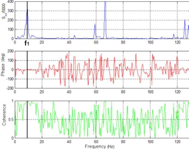
The frequency denoted by f1 appears only at the highest values of the flow coefficient and for

moderately low values of the cavitation number (just before the occurrence of the breakdown). It is related to an axial instability, as clear by analysis of the cross-correlation phase and coherence data presented in Figure 6.5 which shows a phase delay of 0° between the signals from two adjacent transducers at the inlet section and a coherence near to unity. This instability is probably a form of subsynchronous “cavitation surge” with a frequency of about 0.7Ω. Although this form of instability has often been reported to develop together with supersynchronous rotating cavitation, some researchers (Tsujimoto et al., 1997) have also observed it in the absence of supersynchronous phenomena, as in the present case.

The frequency f2 is originated by a single-cell instability rotating in the circumpherential direction.

This conclusion can be drawn from the analysis of the cross-correlation between the signals from the two transducers at the inlet section, which shows a phase delay of about 90° (equal to the angular spacing between the transducers) with a value of the coherence function very close to unity. This instability, being subsynchronous, can probably be attributed to a form of rotating stall, whose occurrence is facilitated by the blunt shape and rough finishing of the blade leading edges. Besides, in the FIP162 inducer the geometry of the three blades is not exactly the same and can easily induce non-uniformities of the flow field, forcing one blade to stall before the others and generating, even without cavitation, the asymmetric blockage typical of rotating instabilities. As a result, flow oscillations appear for practically every value of the flow coefficient, with a frequency of about 0.34Ω that does not seem to depend on the presence of cavitation.

The intensity of this instability decreases for very low values of σ, when the occurrence of generalized cavitation in the inducer inlet interferes with the fluctuations of the cavitation volume associated with the flow instabilities. Note that a similar result, characterized by the detection of a

(6)

rotating stall probably related to the occurrence of strong backflow in the inducer inlet, has been reported by Uchiumi et al. (2002) during the development of the LE-7A liquid hydrogen pump.

The frequency f3 is related to a 0-th order (axial) instability, as can be inferred to Figure 6.6

because the cross-correlation of the two pressure signals at the inlet station has a phase of 0° with unitary coherence function. This instability appears at all values of the flow coefficient with a frequency of about 6÷8 Hz, slightly dependent on the flow coefficient and very close to the expected noncavitating natural frequency of the facility (Saggini, 2004). The instability at frequency f3 is

therefore most likely due to the excitation of the natural mode of oscillation of the flow in the inlet line of the inducer.

The frequencies f4 and f5 are also due to axial instabilities, as shown by Figure 6.7 and Figure 6.8.

The first is a typical cavitation auto-oscillation, whose frequency tends to decrease when the cavitation number is reduced (i.e. for more extensive cavitation). It appears at low values of the cavitation number and for practically every flow coefficient, even if it becomes more intensive for lower flow coefficients. At the lowest values of the flow coefficient and the cavitation number this auto-oscillation leads to a surge-mode instability (frequency f5) characterized by strong axial oscillations at

very low frequency (about 1 Hz). A summary of the flow instabilities detected in the FIP162 inducer is given in Table 6.1.

Figure 6.5 –Power spectrum (blue), phase of the cross-correlation (red) and scaled coherence function (cyan) of the pressure signals from two transducers with 90° angular spacing in the inlet section of the FIP162 inducer at room temperature, 2500 rpm rotating speed, φ = 0.053 and various cavitation numbers.

(7)

(8)

Type of instability Frequency

f1 Cavitation surge 0.7Ω

f2 Rotating stall 0.34Ω

f3 Natural mode of oscillation of the suction line 6÷8 Hz

f4 Cavitation auto-oscillation 1÷6 Hz

f5 Surge 1 Hz

Table 6.1 – Summary of the flow instabilities detected in the FIP162 inducer.

6.2.1 Influence of thermal cavitation effects

Some experiments were carried out at elevated temperature (T = 70 °C) in order to analyze the influence of thermal cavitation effects on cavitation-induced instabilities. The main results obtained from this study are summarized by the two waterfall plots presented in Figure 6.9 and Figure 6.10.

The most significant differences are related to the surge-mode instability (frequency f5) and the

cavitation surge (frequency f1). Comparison of Figure 6.4 and Figure 6.9 shows that the strong

oscillations caused by the surge-mode instability practically disappear at higher temperatures and lower flow coefficients, leading to a flatter spectrum at lower cavitation numbers.

Similarly, comparison of Figure 6.1 and Figure 6.10 shows that the oscillations associated to the cavitation surge instability also tend to become less intense at higher temperatures, moving towards higher values of the cavitation number. The frequency of the oscillations, however, does not seem to depend on the water temperature. No significant temperature-dependent variations have been found for the other detected instabilities (rotating stall, auto-oscillation and the natural mode of the facility), nor any new oscillation phenomena seemed to be detected at higher temperatures.

(9)

Figure 6.9 – Waterfall plot of the power spectrum of the inlet pressure fluctuations in the FIP162 inducer at 70 °C temperature, 2500 rpm rotating speed and φ = 0.008.

Figure 6.10 – Waterfall plot of the power spectrum of the inlet pressure fluctuations in the FIP162 inducer at 70 °C temperature, 2500 rpm rotating speed and φ = 0.057.

6.3 Characterization of the flow instabilities in the MK1 inducer

The characterization of flow instabilities in the MK1 inducer was carried out by installing six piezoelectric transducers at the inducer inlet section and only one transducer at the mid-blade section and one at the outlet section. The azimuthal spacing between the transducers at the inlet axial station

(10)

was 45°. The choice of installing more transducers at the inducer inlet section was driven by the necessity of providing a better characterization of the possible detected rotating instabilities, by means of cross-correlation of more than one couple of signals from different sensors.

A picture of the instrumented Plexiglas section of the facility during the experiments is given in Figure 6.11. As usual, several flow coefficients were investigated. The corresponding waterfall plots, related to the signals from the piezoelectric transducers at the inducer inlet (acquired at a rate of 1000 samples/sec), are presented in the diagrams from Figure 6.12 to Figure 6.15. The Figures show that the rotating frequency Ω was detected together with the blade passing frequency 4Ω. This finding, as in the case of the FIP162 inducer, is an index of asymmetrical cavitation on the four blades of the inducer. However, it can be observed that the peaks corresponding to the rotating frequency are much less evident than in the case of the FIP162 inducer and tend to completely disappear at lower flow coefficients, as expected due to the better geometry and blade finishing of the MK1 inducer.

Figure 6.11 – The Plexiglas inlet section of the facility during the tests for the characterization of the flow instabilities in the MK1 inducer.

Figure 6.12 – Waterfall plot of the power spectrum of the inlet pressure fluctuations in the MK1 inducer at room temperature, 2800 rpm rotating speed and φ = 0.064 (left) and φ = 0.059 (right).

(11)

Figure 6.13 – Waterfall plot of the power spectrum of the inlet pressure fluctuations in the MK1 inducer at room temperature, 2800 rpm rotating speed and φ = 0.0549 (right) and φ = 0.048 (left).

(12)

The first remarkable aspect in the above waterfall plots is that very few oscillation phenomena were found on the MK1 inducer, as expected due to the effective design of this axial pump. The frequency f1 is related to a 0-th order (axial) instability, as can be inferred from Figure 6.16 because

the cross-correlation of the two pressure signals at the inlet station has a phase of 0° with coherence function near to unity. The oscillations were detected at practically all values of the flow coefficient with a frequency of about 8 Hz, slightly dependent on the flow coefficient and very close to the expected noncavitating natural frequency of the facility (Saggini, 2004). As in the case of the FIP162 inducer, this instability is therefore probably due to the excitation of the natural mode of oscillation of the flow in the inlet line of the inducer.

When cavitation becomes more extensive on the inducer blades, the natural mode of frequency f1

tends to transform into a cavitation auto-oscillation (frequency f2), showing the typical frequency

decrease when the cavitation number is reduced. At the lowest values of the flow coefficient and the cavitation number the auto-oscillation leads to a really smooth surge-mode instability (frequency f3)

with a frequency of about 1÷2 Hz. The axial nature of this instability can be deducted by analysis of the phase and coherence function of the cross-correlation, presented in Figure 6.17. Finally it is also possible to observe that at higher flow coefficients, near the nominal operating point of the inducer, the frequency spectrum becomes practically flat, except for the rotational frequency of the pump and its multiples (see Figure 6.12), thus giving a further confirmation of the effectiveness of the MK1 inducer design.

Figure 6.16 –Power spectrum (blue), phase of the cross-correlation (red) and scaled coherence function (cyan) of the pressure signals from two transducers with 45° angular spacing in the inlet section of the MK1 inducer at room temperature, 2800 rpm rotating speed, φ = 0.007 and various cavitation numbers.

(13)

Figure 6.17 –Power spectrum (blue), phase of the cross-correlation (red) and scaled coherence function (cyan) of the pressure signals from two transducers with 45° angular spacing in the inlet section of the MK1 inducer at room temperature, 2800 rpm rotating speed, φ = 0.007 and various cavitation numbers.

A summary of the flow instabilities detected in the MK1 inducer is given in the next Table.

Type of instability Frequency f1 Natural mode of oscillation of the suction line 8 Hz

f2 Cavitation auto-oscillation 2÷8 Hz

f3 Surge 1÷2 Hz

Table 6.2 – Summary of the flow instabilities detected in the MK1 inducer.

6.4 Characterization of the flow instabilities in the FAST2 inducer

The characterization of the flow instabilities in the FAST2 inducer was carried out, similarly to what made for the MK1 inducer, installing six piezoelectric transducers at the inducer inlet section and only one transducer at the mid-blade section and one at the outlet section. The azimuthal spacing between transducers at the inlet axial station was 45°. The inlet section of the facility instrumented with the piezoelectric transducers, with the FAST2 inducer installed, is shown in Figure 6.18.

(14)

Figure 6.18 – The Plexiglas inlet section of the facility instrumented with piezoelectric pressure transducers for the characterization of the flow instabilities in the FAST2 inducer.

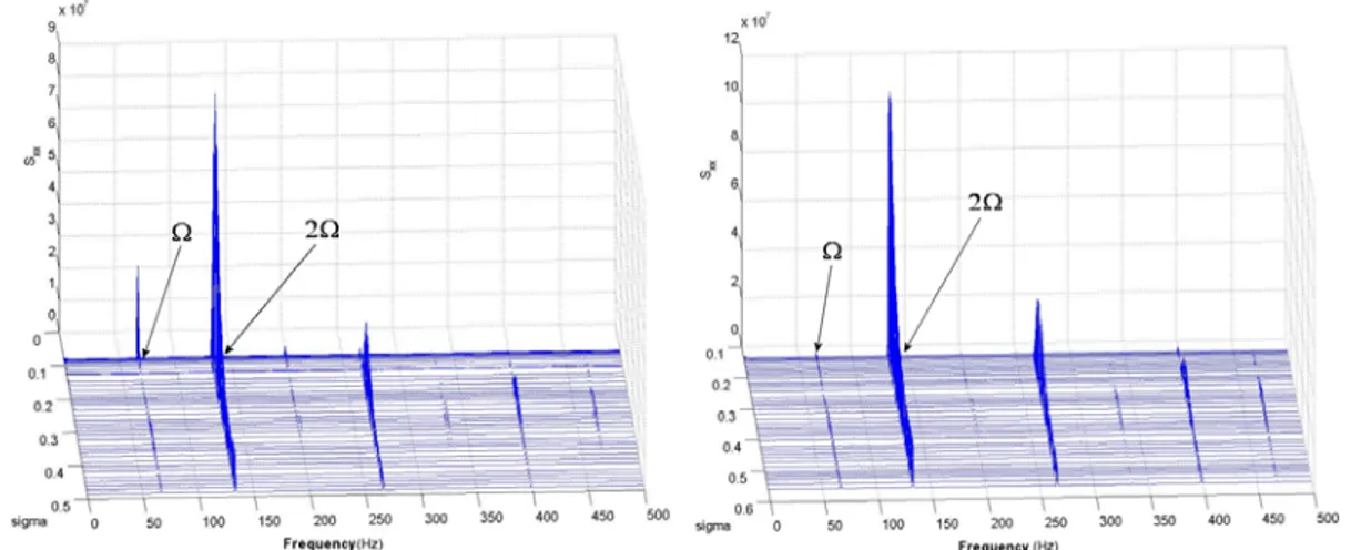
The characteristics of the pressure oscillations generated by the FAST2 inducer under several flow coefficients were investigated. The corresponding waterfall plots, related to signals from the piezoelectric transducers at the inducer inlet (acquired at a rate of 1000 samples/sec), are presented in the diagrams from Figure 6.19 to Figure 6.24. As usual, the rotating frequency Ω was detected together with the blade passing frequency 2Ω, as a consequence of asymmetrical cavitation on the two blades of the inducer.

This was confirmed by optical visualization, which demonstrated the occurrence of cavitating regions characterized by different shape and size on the two blades. As in the case of the MK1 inducer, the peaks corresponding to the rotating frequency are not excessively evident and tend to completely disappear at lower flow coefficients, as a consequence of the well defined geometry and blade finishing of the inducer. It is also noticeable that for φ = 0.07, corresponding to the nominal operating point of the FAST2 inducer, most of the detected flow instabilities which will be illustrated in the following are strongly reduced or even suppressed, thus confirming the effectiveness of the pump design. The waterfall plots show the occurrence of five main instabilities, denoted by frequencies from f1 to f5, whose characteristics and peculiarities will be discussed in the following.

Figure 6.19 – Waterfall plot of the power spectrum of the inlet pressure fluctuations in the FAST2 inducer at room temperature, 4000 rpm rotating speed and φ = 0.09 (left) and 0.083 (right).

(15)

Figure 6.20 – Waterfall plot of the power spectrum of the inlet pressure fluctuations in the FAST2 inducer at room temperature, 4000 rpm rotating speed and φ = 0.076 (left) and φ = 0.07 (right).

(16)

Figure 6.24 – Waterfall plot of the power spectrum of the inlet pressure fluctuations in the FAST2 inducer at room temperature, 4000 rpm rotating speed and φ = 0.01.

A particularly interesting version of the above presented waterfall plots can be obtained by means of two analytical manipulations. The first of these modifications consists in carrying out a digital filtering of the piezoelectric transducers signals during their post-processing, in order to eliminate the rotating frequency Ω and its multiples. This result can be accomplished using a notch filter, which gives the possibility to attenuate the power spectrum peaks corresponding to really narrow frequency bands. This technique is particularly useful because the peaks related to the rotating frequency and its multiples are usually much more significant than the ones related to the other instabilities. Elimination of these peaks could therefore lead to the detection of other “secondary” instabilities, as will be briefly showed in the next section. The second modification consists in showing the real amplitude of pressure fluctuations, instead of their power spectrum, on the z-axis of the waterfall plots. The relation between the real amplitude and the power spectrum of the fluctuations is obviously quadratic. As a consequence, when applied to waterfall plots like the ones of the preceding Figures, it tends to “highlight” less intensive frequencies with respect to the more evident ones. Note that the application of this technique can be helpful, as for the filtering of rotating frequency and its multiples, in order to detect the occurrence of possible secondary instabilities. Figure 6.25 shows the waterfall plots of the

(17)

Figure 6.25 – Waterfall plot of the real amplitude of inlet pressure fluctuations in the FAST2 inducer at room temperature, 4000 rpm rotating speed and φ = 0.09 (left) and φ = 0.01 (right). A digital notch filter

has been applied to eliminate the rotating frequency and its multiples.

The instability denoted by f1 has the typical characteristics of a cavitation auto-oscillation. It can

be easily recognized as an axial instability, as evident in Figure 6.26 and Figure 6.27 which show that the phase of the cross-correlation between the signals from couples of transducers at different angular spacing in the inlet section is equal to 0° and the coherence function is unitary.

The frequency f1 is in the range 5÷12 Hz and tends to decrease when cavitation number is reduced

(i.e. for more extensive cavitation). This instability appears at low values of the cavitation number and for practically every flow coefficient, even if it becomes more intensive for lower flow coefficients.

The frequency f2 is also related to an axial instability, as clearly shown by analysis of the phase

and coherence function of cross-correlation between different couples of transducers, presented in Figure 6.28 and Figure 6.29. The phenomenon denoted by f2 is observed for all the values of φ, but

tends to become more significant at higher flow coefficients. Its amplitude tends to decrease at lower cavitation numbers. The frequency is about 4.4 times the pump rotational speed. This instability has characteristics very similar to those of the high-order cavitation surge instabilities recently observed by Tsujimoto and Semenov (2002) on the Japanese LE-7 inducers, whose frequency has been reported to be in the range from 4 to 5 times the pump rotational speed.

The frequency f3 is related to an axial phenomenon (see Figure 6.30 and Figure 6.31), having the

same characteristics of the f2 instability. This finding, together with the strong frequency correlation

(the value of f3 is exactly equal to 1.5 times f2) leads to the conclusion that the two frequencies are

probably due to the same form of instability.

Finally, the frequencies f4 and f5 are related to single-cell rotating instabilities. This conclusion can

be drawn by examination of the waterfall plots presented from Figure 6.32 to Figure 6.36, which show a phase delay between two transducers at the inducer inlet section equal to their angular spacing, with a value of the coherence function very close to unity. Note that this behaviour was observed for various couples of piezoelectric transducers, separated by different angular spacing.

These two rotating phenomena become significant at lower values of the flow coefficient, with frequencies f4 = 0.31Ω and f5 = 1.69Ω, symmetrically located above and below the rotating speed.

(18)

The frequency f4 tends to decrease slightly (and, correspondingly, f5 slightly increases) at very low

values of the cavitation number. The subsynchronous instability denoted by f4 can probably be

attributed to a form of rotating stall, similar to the one observed in the FIP162 inducer. In the case of the FAST2 inducer, the rotating stall detected at lower flow coefficients is probably caused by the occurrence of strong backflow in the inducer inlet, in a similar way to what reported by Uchiumi et al. (2002) to be found during the development of the LE-7A liquid hydrogen pump. At the same time, at low flow coefficients and high incidence angles the inducer works near stalled conditions and so one blade is facilitated to stall before the other, leading to the detected rotating instability. The supersynchronous f5 frequency is probably related to the same instability phenomenon which moves

simultaneously in two directions, the same of the rotating pump (leading to f5 frequency) and the

opposite one (leading to f4 frequency). Table 6.3 gives a summary of the main flow instabilities

detected in the FAST2 inducer.

Figure 6.26 –Power spectrum (blue), phase of the cross-correlation (red) and coherence function (green) of the pressure signals from two transducers with 45° angular spacing in the inlet section of the FAST2 inducer at room temperature, 4000 rpm rotating speed, φ = 0.09 and σ = 0.161(left) and σ = 0.09 (right).

Figure 6.27 –Power spectrum (blue), phase of the cross-correlation (red) and coherence function (green) of the pressure signals from two transducers with 135° angular spacing in the inlet section of the FAST2

(19)

Figure 6.28 –Power spectrum (blue), phase of the cross-correlation (red) and coherence function (green) of the pressure signals from two transducers with 45° angular spacing in the inlet section of the FAST2 inducer at room temperature, 4000 rpm rotating speed, φ = 0.09 and σ = 0.296 (left) and σ = 0.19(right).

inducer at room temperature, 4000 rpm rotating speed, φ = 0.09 and σ = 0.405.

(20)

(21)

(22)

Type of instability Frequency

f1 Cavitation auto-oscillation 5÷12 Hz

f2 High-order cavitation surge 4.4Ω

f3 High-order cavitation surge (?) 6.6Ω

f4 Rotating stall

(moving in opposite direction to the pump)

0.31Ω f5 Rotating stall

(moving in the same direction of the pump)

1.69Ω

Table 6.3 – Summary of the flow instabilities detected in the FAST2 inducer.

6.4.1 Investigation of secondary flow instabilities

The filtering of frequency spectra and the consequent elimination of the peaks corresponding to the rotating frequency and its multiples, as anticipated before, gave the possibility to highlight some less evident peaks in the waterfall plots. A number of “secondary” flow instabilities were therefore identified, some of which will be discussed in this Section.

It has to be observed that these secondary instabilities are related to very weak phenomena, and it is particularly difficult to extract the relevant information about their axial or azimuthal nature from the cross-correlation plots. Only for few of the detected oscillations it is possible to postulate some conclusions abut their nature and characteristics, as illustrated in the following.

The waterfall plots of the filtered power spectra, for two particular values of the flow coefficient, are showed in Figure 6.37 and Figure 6.38. The frequencies of all the observed secondary oscillating phenomena are highlighted in the Figures.

Figure 6.37 – Waterfall plot of the filtered power spectrum of inlet pressure fluctuations in the FAST2 inducer at room temperature, 4000 rpm rotating speed and φ = 0.09.

(23)

Figure 6.38 – Waterfall plot of the filtered power spectrum of inlet pressure fluctuations in the FAST2 inducer at room temperature, 4000 rpm rotating speed and φ = 0.01.

The four instabilities for which some conclusions could be drawn have been denoted by frequencies from f6 to f9. The phenomenon denoted by f6 was detected at every value of the flow

coefficient. It is related to an axial phenomenon, as can be inferred from analysis of the phase and coherence function of the cross-correlation, showed in Figure 6.39. The frequency is equal to about 304 Hz (4.6Ω). The phenomenon f7 also seems to be related to an axial phenomenon, as shown by

Figure 6.40. It was observed at higher values of the flow coefficient, and the related frequency was about 496 Hz (7.4Ω). The frequency f8, equal to 378 Hz (5.6Ω), has been found to be related to a

rotating phenomenon, detected only at lower flow coefficients. Analysis of Figure 6.41 seems to show that the phase of the cross-correlation between the signals from two transducers is three times the angular separation of the transducers. As a consequence, the phenomenon denoted by f8 is most likely

due to a weak azimuthal instability characterized by three rotating cells. The real frequency of this oscillation is therefore equal to 378 / 3 = 126 Hz (1.9Ω). The frequency f9, equal to 488 Hz (7.3Ω), can

be associated to a single-cell rotating instability, as shown by Figure 6.42. It was detected only at lower values of the flow coefficient. The characteristics of the secondary flow instabilities detected in the FAST2 inducer are summarized in Table 6.4.

(24)

(25)

Type of instability Field of existence Frequency

f6 Axial oscillation Every value of φ 4.6Ω

f7 Axial oscillation Higher flow coefficients 7.4Ω

f8 Three-cells rotating instability Lower flow coefficients 1.9Ω

f9 Single-cell rotating instability Lower flow coefficients 7.3Ω

Table 6.4 – Characteristics of the secondary flow instabilities detected in the FAST2 inducer.

6.5 Summary of the detected instabilities

The following Table presents a summary of the instabilities that have been detected testing the FIP162, the MK1 and FAST2 inducers.

Type of instability FIP162 MK1 FAST2

Cavitation surge x

Rotating stall x x

Natural mode of oscillation of the suction line x x

Cavitation auto-oscillation x x x

Surge x x

High-order cavitation surge x

(26)

6.6 High speed camera experimental tests

Gas-liquid flows, characterized by turbulence, deformable phase interface, phase interaction and cavitation instabilities are extremely difficult to model. Flow visualization provides effective means to obtain both quantitative and qualitative information from complex fluid flow. The use of a high speed camera allows validating and further analysing the cavitation phenomenon as well as flow instabilities through the comparison of the experimental results obtained by the cross-correlation analysis of the piezoelectric transducers signals, presented in the last paragraphs, and the images. This section is dedicated to the description of the integrated system for the optical visualization and to the study of cavitation developed on the FAST2 and the FIP162 inducers through the accurate analysis of the frames.

6.6.1 Integrated system for the optical analysis of the cavitating flow

The flow images are obtained using a high-speed digital imaging system

The integrated system for the optical analysis of the cavitating flow is composed by the following items:

− A Nikon Coolpix 5700 digital photo camera with the following specifications: → Number of pixels: 5 millions (maximum image size 2560x1920) → Lens: Zoom 8x, focal 8.9-71.2 mm

→ Digital zoom: 4x

→ Shutter speed: from 1/4000 sec to 8 sec.

− A stroboscopic light Drelloscop 3009, with the following specifications: → Flash frequency: from 0.5 to 1000 lamps/second

→ Frequency accuracy: 0.001%

→ Flash energy: max 0.35 Ws Joule/flash (depending on the flash frequency) → Flash frequency can be controlled by external trigger signals

− Three halogen lamps produced by Hedler, each one having a power of 1250 W

− A high-speed video camera, Fastec Imaging model Ranger, having the following specifications:

→ Recording rate: from 125 frames/second (max resolution 1280x1024) to 16000 frames/second (max resolution 1280x32)

→ Maximum resolution at 1000 frames/seconds: 640x480 → Maximum resolution at 4000 frames/second: 1280x128 → Sensor: CMOS array, up to 1280x1024 pixels, monochrome → Shutter speed: from 1x to 20x the recording rate

→ Recording mode: manual or trigger

→ Playback rate: from 1 frame/second d to 1000 frames/second → Personal Computer connection by means of USB port → Trigger input: Contact Closure or standard TTL signal → Standard C-mount lens mount

The system records a sequence of digital images of the flow at a pre-selected frame rate and stores the frames in an image memory on the controller unit. The images can be viewed at any selected frame rate, frame by frame or freeze frame, to analyse flow motion and time during the sequence. With an increase in frame rate, image pixel resolution is reduced (Figure 6.43); consequently it is necessary to optimize the frame rate with the flow conditions.

(27)

Figure 6.43 – High Speed camera data sheet

− Three halogen lamps produced by Hedler, each one having a power of 1250 W. − A Nikon Coolpix 5700 digital photo camera with the following specifications:

→ Number of pixels: 5 millions (maximum image size 2560x1920) → Lens: Zoom 8x, focal 8.9-71.2 mm

→ Digital zoom: 4x

→ Shutter speed: from 1/4000 sec to 8 sec.

− A stroboscopic light Drelloscop 3009, with the following specifications: → Flash frequency: from 0.5 to 1000 lamps/second

→ Frequency accuracy: 0.001%

→ Flash energy: max 0.35 Ws Joule/flash (depending on the flash frequency) → Flash frequency can be controlled by external trigger signals.

The next Figure shows the integrated system (in particular, the high-speed video camera and the three halogen lamps) installed for the visualization of the cavitating flow in the FAST2 inducer. The halogen lamps and the high- speed camera were accurately positioned in order to assure the best optic set up in respect to the camera sensor and the lamps illumination.

(28)

Figure 6.44 – Picture of the high-speed video camera and the halogen lamps installed in the facility.

Figure 6.45 – Successive frames of the FAST2 inducer taken at a frame rate of 1000 fps (φ = 0.07, σ = 0.14).

(29)

Figure 6.47 – Successive frames of the FAST2 inducer taken at a frame rate of 1000 fps (φ = 0.008, σ = 0.3).

6.6.2 Image Processing Algorithm

An image processing algorithm has been developed to characterize the regions of the image where cavitation is present. This algorithm has been implemented in a code that allows for automatically processing the frames of the movies taken by the high-speed camera and for analyzing the movie using the processed frames. The algorithm has been implemented in Matlab®_{and its flow chart is shown in}

Figure 6.48. The input is a frame in gray-scale format: a typical input frontal image is shown in Figure 6.49 (a) whereas a typical input side image is shown in Figure 6.50 (left).

(30)

(a) (b)

Figure 6.49 – Comparison between the original frame (a) and the processed binary image (b) in a sample case.

Figure 6.50 – Selection of the cavitating area on a grayscale image (left), luminosity histogram (center) and binarized image (right). Inducer: FAST2, Flow conditions: Ф = 0.04

It is important to identify the position of the inducer rotational axis with good precision in every frame, in order to rotate all the processed frames around this point and obtain a movie in which the position of the blades is fixed. It is therefore possible to characterize the development of the cavitating surface on the blades in order to detect possible oscillations. The rotational axis is manually selected on the image, while the angle of rotation of every frame around this point can be simply calculated as a function of the inducer rotational speed and the sample rate at which the movie has been taken.

The next step of the algorithm is the so-called “segmentation technique”, by which the cavitating regions are separated by the rest of the image. Several segmentation techniques have been proposed in the past by the open literature (see for example Gonzales, 2002), but the most widely used are the edge detection algorithms and the thresholding technique (see respectively Hiscock et al., Kato et al.). In the present paper, the thresholding technique has been used. By this technique, the original grayscale image is converted in a binary image: the pixels having an intensity in the original image greater than a certain threshold value are set equal to 1 (i.e., they become white pixels), while all other pixels are set equal to 0 (i.e., they become black pixels). Despite its implementation simplicity, the main problem of this technique is the evaluation of the right value to be attributed to the threshold. There are several methods to automatically find this value according to the image histogram properties (Gonzalez, 2002, Kato et al., Otsu, 1979). Typical luminosity histograms of the cavitating areas show double peaks and a good choice for the threshold value is represented by the value between the peaks (Figure 6.50).

Sometimes the histogram does not show two clearly distinguished peaks and the threshold value can then be found by a trial-and-error technique until the right value is found (i.e. the value that

(31)

the angular division of the frame it is possible to obtain two well distinguished peaks in the histogram for each sector. This allows for obtaining a good first-tentative image segmentation. In order to better analyze the cavitating regions on the blades, the central portion of the image (where other cavitating phenomena often occur) and the region outside the inducer are covered with black pixels (masked portions in Figure 6.51). If the white regions in the first-tentative binarized image do not superimpose to the effective cavitating regions of the original frame, the operator can manually process the frame selecting the right cavitating areas and a new threshold value.

Figure 6.51 – Example of the image division and the masked portions.

(32)

6.6.2.1 Results

Procedure

The working fluid has been deareated before every test. In order to improve the image quality, excessively high cavitation levels have not been reached during the tests. For this reason, the inducer rotational speed has been set equal to 1500 rpm. High speed movies have been recorded at constant flow rate, while the inducer inlet pressure has been decreased from high to low values using the vacuum pump.

The camera frame rate has been set equal to 1000 fps (i.e. 40 frames/revolution at 1500 rpm), at an image resolution of 640x480 pixels. This setup gave the possibility of optically analyzing the cavitation instabilities previously detected on the same inducer by unsteady pressure measurement analysis.

Analysis of the cavitating surface on the blades

The first plot, presented in Figure 6.53 (a), shows the normalized frontal cavitating surface as a function of the flow coefficient for several cavitation numbers. The total frontal area of the cavitating regions on the inducer blades (Scav) has been estimated by mediating the number of white pixels in all

the frames of a movie taken at given flow conditions. This value has been normalized using the total frontal area of the inducer (Sflow).

0 0.01 0.02 0.03 0.04 0.05 0.06 0.07 0.02 0.04 0.06 0.08 0.1 0.12 0.14 Φ Sca v /S flo w σ=0.60 σ=0.48 σ=0.45 0.4 0.45 0.5 0.55 0.6 0.65 0.02 0.04 0.06 0.08 0.1 0.12 0.14 σ Sca v /S flo w Φ=0.060 Φ=0.057 Φ=0.053 Φ=0.040 Φ=0.034 Φ=0.029 Φ=0.008 (a) (b)

Figure 6.53 – Flow chart of the semi-automatic algorithm.

By examination of Figure 6.53 (a) it can be observed that the cavitating surface tends to decrease when the flow coefficient decreases. At lower flow coefficients and cavitation numbers, the image processing algorithm described in the previous Section can not be used properly, due to the significant number of vortices and large cavitation regions in the inducer inlet flow. The water quality is significantly degraded, with a large number of cavitating nuclei and consequently adverse effects on light diffusion (Figure 6.54).

(33)

In the plot of Figure 6.53 (a) it can also be observed that the cavitating surface tends to decrease when the cavitation number increases. This phenomenon also shown by Figure 6.53 (b), where the normalized frontal area of the cavitating surface is shown as a function of the cavitation number for several flow coefficients. This aspect is evident by observation of the frames shown in Figure 6.55 and referred to a particular value of the flow coefficient.

Figure 6.55 –Development of cavitation on the FIP162 inducer

Tip cavity length estimation

The tip cavity length has been estimated using an automatic algorithm which scans every binarized frame with a line rotating around the inducer axis with an angular pitch of 1°. When a white pixel is found along the scanning line after a completely black line, the cavitating region is assumed to begin; on the other hand, when every pixel along the scanning line becomes black, the cavitating region is assumed to finish (Figure 6.56).

The length of the cavitating region is finally estimated by multiplying the azimuthal extension ∆θ by the radius at which the cavitating region has been examined. This procedure has been applied to a binarized movie whose frames have been rotated around the inducer rotational axis in order to obtain fixed blade position.

(34)

Figure 6.56 – Evaluation of the azimuthal extension of the cavitation on a blade

The following plots (Figure 6.57) show the length of the cavitating region on the blades as a function of time, for given flow conditions.

Sometimes the cavitating region appears to be fragmented. This is due to the separation of small cavitating regions and to the presence of vortexes between the real blade surface and the camera lens, as shown in Figure 6.54. In this case the algorithm takes into account the angular separation between the different cavitating regions and, if they are sufficiently close, they are considered as an unique cavitating region. Otherwise, if the cavitating regions are sufficiently distant, they are considered as effectively separated and only the length of the first one is taken into account.

0 0.02 0.04 0.06 0.08 0.1 0.12 0.14 0.16 0.18 0.2 0.6 0.8 1 1.2 1.4 Time [s] T ip C a vi ty L e n g th /Pi tc h Blade n°1 0 0.02 0.04 0.06 0.08 0.1 0.12 0.14 0.16 0.18 0.2 0.5 1 1.5 Time [s] T ip C a v ity L e n g th /P it ch _{Blade n°2} 0 0.02 0.04 0.06 0.08 0.1 0.12 0.14 0.16 0.18 0.2 0 0.5 1 1.5 2 Time [s] T ip C a v it y Le ngt h /P it c h Blade n°3

Figure 6.57 – Evaluation of the azimuthal extension of the cavitation on a blade

Sometimes the cavitating region appears to be fragmented. This is due to the separation of small cavitating regions and to the presence of vortexes between the real blade surface and the camera lens, as shown in Figure 6.54. In this case the algorithm takes into account the angular separation between the different cavitating regions and, if they are sufficiently close, they are considered as an unique cavitating region. Otherwise, if the cavitating regions are sufficiently distant, they are considered as effectively separated and only the length of the first one is taken into account.

(35)

0 50 100 150 200 -200 0 P hase [deg 0 50 100 150 200 -200 0 200 P h as e [ deg] 0 50 100 150 200 -200 0 200 Frequency [Hz] P hase [de g ]

Figure 6.58 – Power spectrum of the tip cavity length on third blade (blue). Phase of the cross-correlation between 3rd_{and 2}nd_{blade (second plot), 2}nd_{and 1}st_{blade (third plot), 1}st_{and 3}rd_{blade (fourth plot).}

As shown in Figure 6.58, a well defined peak is detected in the power spectrum at a frequency of 15.7 Hz (f1). The detected rotating stall had a frequency of about 0.34Ω in a fixed coordinate frame (8.5 Hz at 1500 rpm). In a coordinate frame rotating with the blades (as the one used to estimate the cavity length) this frequency becomes 16.5 Hz, very close to the value of f1. Figure 6.58 shows that the cross-correlation phases are 116° (blade 3-blade 2), 160° (blade 2-blade 1) and 87° (blade 1-blade 3). This means that the phenomenon is rotating clockwise in the rotating coordinate frame. The ratio of the mean angular separation of two adjacent cavitating regions to the relative cross-correlation phase is about one and this means that the oscillation involves just one single rotating cell. From these results, it is clear that the instability denoted by f1 has characteristics similar to the rotating stall previously

detected on the same inducer.

Figure 6.59 (a) shows a sinusoidal signal at frequency f1, whose magnitude and phase have been

calculated using a trial-and-error technique, superimposed to the non-dimensional tip cavity length on the third blade, while Figure 6.59 (b) shows the same sinusoidal signal shifted of an angle equal to the phase of the cross-correlation between blade 3 and blade 1. Figure 6.60 (a) shows the sinusoidal signals of Figure 6.59 together with that obtained for the remaining blade (same frequency, phase calculated from the cross-correlation analysis): the cavity propagates clockwise from the first blade to the third blade. It is also evident that the mean cavity length on the third blade is lower than the other two (asymmetric cavitation, Figure 6.60 (b)).

(36)

0 0.05 0.1 0.15 0.2 0.2 0.4 0.6 0.8 1 1.2 1.4 1.6 Time [s] T ip C a v it y Len gt h/ P it c h Blade n°3 A 3sin(2πf1t+φ3) 0 0.05 0.1 0.15 0.2 0.6 0.7 0.8 0.9 1 1.1 1.2 1.3 1.4 Time [s] T ip C a v ity L e n g th /P it c h Blade n°1 A₁sin(2πf₁t+φ₁)

Figure 6.59 – Sinusoidal signal at frequency f1 superimposed to the measured non-dimensional

0 0.05 0.1 0.15 0.2 0.4 0.5 0.6 0.7 0.8 0.9 1 1.1 1.2 1.3 Time [s] T ip C a v it y Le ngth/P itc h Blade n°1 Blade n°2 Blade n°3 3 2 1

Figure 6.60 – Oscillation of the cavity length on the blades of the FIP inducer (a). Example of asymmetric blade cavitation (b).

6.6.3 Conclusion

The research activity has allowed for the development and successful validation of a viable and effective tool, based on optical processing of high-speed video movies for quantitative analysis and diagnostics of cavitation instabilities in turbopump inducers. The capabilities of the semi-automatic algorithm created to implement the proposed technique have been improved by developing a procedure for the estimation of the frontal cavitating surface and the extension of the cavitating regions on the blades. Preliminary application of the above technique to the analysis of cavitation in a test inducer lead to the detection of the same rotating stall instability previously observed under the same operating conditions by means of Fourier analysis of the inlet pressure signals. The results confirm the potential of the proposed method in the characterization of cavitation-induced instabilities and suggest the possibility of extracting additional useful information on the nature, extent and location of the cavitating regions on the inducer blades by means of more spatially-resolved processing of the video images.