3. EXPERIMENTAL RESULTS AND MACROSCOPIC STRUCTURE OF THE AIR-WATER FLOW 3.1 Presentation

3. EXPERIMENTAL RESULTS AND MACROSCOPIC STRUCTURE OF THE

AIR-WATER FLOW

3.1 Presentation

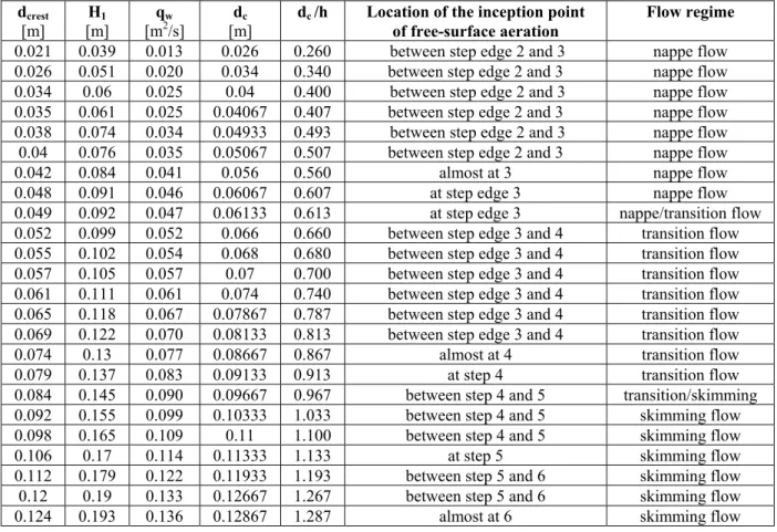
The basic flow regimes were observed in a series of preliminary experiments with discharges ranging from 0.013 to 0.136 m3_{/s. Visual observations were complemented by photographic information. All}

data are summarized in Table 3-1 where dcrest is the flow depth measured above the weir crest, H1 is the

upstream total head measured above the weir crest, qw is the water discharge per unit width, dc is the

critical flow depth and h is the step height. dcrest

[m] [m] H1 [mq2w _{/s] [m]} dc dc /h Location of the inception point _{of free-surface aeration} Flow regime 0.021 0.039 0.013 0.026 0.260 between step edge 2 and 3 nappe flow 0.026 0.051 0.020 0.034 0.340 between step edge 2 and 3 nappe flow 0.034 0.06 0.025 0.04 0.400 between step edge 2 and 3 nappe flow 0.035 0.061 0.025 0.04067 0.407 between step edge 2 and 3 nappe flow 0.038 0.074 0.034 0.04933 0.493 between step edge 2 and 3 nappe flow 0.04 0.076 0.035 0.05067 0.507 between step edge 2 and 3 nappe flow 0.042 0.084 0.041 0.056 0.560 almost at 3 nappe flow 0.048 0.091 0.046 0.06067 0.607 at step edge 3 nappe flow 0.049 0.092 0.047 0.06133 0.613 at step edge 3 nappe/transition flow 0.052 0.099 0.052 0.066 0.660 between step edge 3 and 4 transition flow 0.055 0.102 0.054 0.068 0.680 between step edge 3 and 4 transition flow 0.057 0.105 0.057 0.07 0.700 between step edge 3 and 4 transition flow 0.061 0.111 0.061 0.074 0.740 between step edge 3 and 4 transition flow 0.065 0.118 0.067 0.07867 0.787 between step edge 3 and 4 transition flow 0.069 0.122 0.070 0.08133 0.813 between step edge 3 and 4 transition flow 0.074 0.13 0.077 0.08667 0.867 almost at 4 transition flow 0.079 0.137 0.083 0.09133 0.913 at step 4 transition flow 0.084 0.145 0.090 0.09667 0.967 between step 4 and 5 transition/skimming 0.092 0.155 0.099 0.10333 1.033 between step 4 and 5 skimming flow 0.098 0.165 0.109 0.11 1.100 between step 4 and 5 skimming flow 0.106 0.17 0.114 0.11333 1.133 at step 5 skimming flow 0.112 0.179 0.122 0.11933 1.193 between step 5 and 6 skimming flow 0.12 0.19 0.133 0.12667 1.267 between step 5 and 6 skimming flow 0.124 0.193 0.136 0.12867 1.287 almost at 6 skimming flow

Table 3-1 Summary of flow regime observations

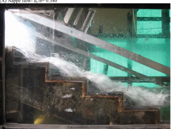
For small flow rates (dc/h < 0.5), the waters flowed as a succession of free-falling jets that was typical

of a nappe regime (Figure 3.1A). For some intermediate discharges (0.5 < dc/h < 0.95), a transition

flow regime was observed. The flow was very chaotic: it was characterized by strong splashing and by many droplets’ ejections downstream of the inception point (Figure 3.1B). For larger flow rates (dc/h >

0.95), the waters skimmed above the pseudo-bottom formed by the steps edges. The skimming flows were characterised by strong cavity recirculation with three-dimensional vertical patterns (Figure 3.1C).

Figure 3.1- Photographs of nappe, transition and skimming flow regimes.

(A) Nappe flow- dc/h= 0.340

(C) Skimming flow- dc/h= 1.287

The location of the inception point of free-surface aeration was found by visual observations and it is defined as the place where free surface became white (Figure 3.2). Its location was recorded for all discharges (Table 3-1, Figure 3-3). In Figure 3.3, the data are presented as LI/ks as function of F*,

where LI is the streamwise distance from step edge one and ks is the step cavity height normal to the

flow direction calculated as ks=h*cosθ. F* is a Froude number defined as:

* w 3

q

F

g sin

(h cos )

=

⋅

θ⋅ ⋅

θ

where qw is the water discharge per unit width, g is the gravity acceleration and θis the angle between

the pseudo bottom and the horizontal. The data were best fitted by:

* I

L

1.05 5.11 F

h cos

⋅

θ

=

+

⋅

The present data are compared in Figure 3.3 with earlier data with smooth steps (GONZALEZ et al.2005) and a study with rough steps (GONZALEZ et al. 2005), as well as the empirical correlation of CHANSON (1995): 1.4 0.111 * I

L

24.14 sin( )

F

h cos

⎛

_{⎞ =}

_⋅

_θ

_⋅

⎜

_⋅

_θ

⎟

⎝

⎠

Figure 3.2- Photograph of white waters looking downstream. Flow rate: dc/h= 1.45 0 5 10 15 20 0 0.5 1 1.5 _Fr* 2 2.5 3 3.5 4 LI /k s

LI/ks Present study

LI/ks CM H_05 Rough steps LI/ks CM H_05 Smooth steps 1.05+5.11*F*

Correlation CHANSON (1995)

Figure 3.3- Dimensionless location of the inception point of free-surface aeration and empirical correlations (Eq. 3-2 and Eq. 3-3).

Five discharges were selected to investigate the air-water flow properties. For the flow rates dc/h=1.0,

dc/h=1.33 and dc/h=1.57 a single-tip conductivity probe was used. For two intermediate discharges

(dc/h=1.15 and for dc/h=1.45), two single-tip conductivity probes were utilized. The probe sensors

were located at the same longitudinal and normal location x and y respectively, but they were separated by a known transverse distance z. For these two discharges two different double-tip probes were used to investigate the flow in longitudinal direction. Table 3-2 summarises the experimental flow conditions.

dc/h Location of the _{inception point} Step edge _No. Probes and geometry Flow regime

1.0 between step 5 and 6 6,7,8,9,10 single-tip probe [Ø=0.35 mm ] _{skimming flow} Transition- 7 two single-tip probes [Ø=0.35 mm ] _{z=8.45 mm}

8 two single-tip probes [Ø=0.35 mm ] _{z=8.45 mm} 9 two single-tip probes [Ø=0.35 mm ] _{z=8.45 mm} two single-tip probes [Ø=0.35 mm ]

z=3.6 mm z=6.3 mm z=8.45 mm z=10.75 mm z=13.7 mm z=16.7 mm z=21.7 mm z=29.5 mm z=40.3 mm 1.15 _{step 6 and 7} between

10 double-tip probe [Ø=0.25 mm] ∆x=7 mm and ∆x=9.6 mm ∆z=1.4 mm Skimming flow single-tip probe [Ø=0.35 mm ]

1.33 between step 6 and 7 7,8,9,10 _{double-tip probe [Ø=0.35 mm ]} Skimming flow 8 two single-tip probes [Ø=0.35 mm ] _{z=8.45 mm}

9 two single-tip probes [Ø=0.35 mm ] _{z=8.45 mm} two single-tip probes [Ø=0.35 mm ]

z=3.6 mm z=8.45 mm z=13.7 mm z=21.7 mm z=40.3 mm z=55.7 mm 1.45 _{step 7 and 8} between

10

double-tip probe [Ø=0.25 mm] ∆x=7 mm and ∆x=9.6 mm,

∆z=1.4 mm

Skimming flow

1.57 between step 7 and 8 8,9,10 single tip probe [Ø=0.35 mm ] Skimming flow Table 3-2 Summary of the flow conditions for air-water flow measurements

3.2 Flow properties

Several parameters were used to characterise the aerated flow properties: air concentration or void fraction, bubble count rate, velocity, turbulence intensity.

3.2.1 Void fraction and bubble count rate distributions

Both single-tip and double-tip conductivity probes provided void fraction data. Measurements were conducted at step edges For different flow rates the profiles showed the same pattern. This is shown in Figures 3.1. The data are presented in dimensionless terms: the void fraction as function of y/Y90

where y is the distance from the pseudo-bottom and Y90 is the characteristic depth where the air

concentration is 90% calculated by linear interpolation.

0 0.5 1 1.5 2 2.5 0 0.1 0.2 0.3 0.4 _C 0.5 0.6 0.7 0.8 0.9 1 y/ Y 90 Step 8 dc/h=1.0 Step 10 dc/h=1.0 Step 8 dc/h=1.56 Step 10 dc/h=1.56

T heory Step10 dc/h=1.56 CHANSON and T OOMBES 2001

Figure 3.4 – Dimensionless void fraction distribution Flow rates: dc/h=1.0, dc/h=1.57.

Instrumentation: single-tip probe [Ø=0.35 mm]. Comparison with Equation (3-4).

The air concentration distribution followed closely the analytical expression developed by CHANSON and TOOMBES (2001): 3 2 0 0 1 y ' y ' 3 C 1 tanh K '' 2 D 3 D ⎛ _{⎛ ⎞} ⎞ − ⎜ _{⎜ ⎟} ⎟ ⎝ ⎠ ⎜ ⎟ = − − + ⎜ ⋅ ⋅ ⎟ ⎜ ⎟ ⎜ ⎟ ⎝ ⎠ (3-4)

where: y’=y/Y90 * 0 0

1

8

K '' K

2D

81D

=

+

−

C

=

0.7622(1.0434 e

−

)

90 Y

mean 0

C =

_∫

longitudinal distance x/dc where x is the streamwise distance from step edge one, dc is the critical

depth. Note in Figure 3-5, the rapid increase in mean void fraction immediately downstream of the inception point. 0 0.1 0.2 0.3 0.4 0.5 0.6 0 5 10 x/dc 15 20 25 Cm ea n Cmean dc/h=1.0 Cmean dc/h=1.15 Cmean dc/h=1.33 Cmean dc/h=1.45 Cmean dc/h=1.56 inception

Figure 3.5 – Mean air content Cmean Flow rates: dc/h=1.0, dc/h=1.15, dc/h=1.33, dc/h=1.45, dc/h=1.57.

Instrumentation: single-tip probe [Ø=0.35 mm].

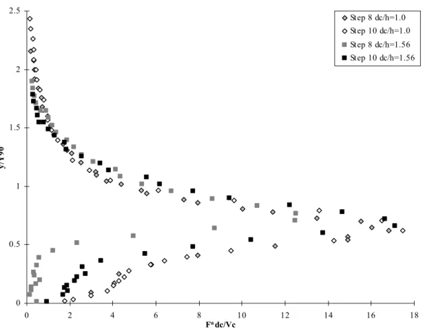
All discharges were characterized by high level of air entrainment and bubble counts. This was observed with the bubble count rate distributions. The bubble count rate (F) is defined as the number of bubbles/droplets per second. It is presented with F·dc/Vc as a function of y/Y90 where dc is the

critical flow depth and Vc is the critical velocity (Figure 3.6).

The relationship between the bubble count rate and void fraction tended to be parabolic. For all discharges the data were fitted by a parabolic law (CHANSON 1997, International Journal of Multiphase Flow):

max

F

4 C (1 C)

F

= ⋅ ⋅ −

where:

C is the void fraction

Fmax is the maximum bubble count rate in the cross section

Eq. (3-6) is shown in Figure 3.7.

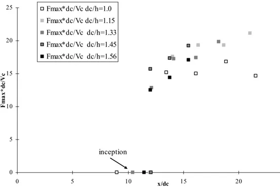
For all discharges, the data showed that the bubble count rate reached its maximum for values of void fraction between 0.4 and 0.5 (Figure 3.7, Table 3-2). Table 3-2 summarises the flow properties at the locations y=ymax where F=Fmax. Fmax is presented in dimensionless terms, Fmax·dc/Vc, as a function of

x/dc in Figure 3.8. Fmax·dc/Vc is fairly constant for the lowest discharge (dc/h=1.0) but it is increasing

for the other flow rates. For these discharges, Fmax·dc/Vc is directly proportional to x/dc and the greater

is the flow rate, the steeper is the increase.

0 0.5 1 1.5 2 2.5 0 2 4 6 8 10 12 14 16 18 F*dc/Vc y/ Y 90 Step 8 dc/h=1.0 Step 10 dc/h=1.0 Step 8 dc/h=1.56 Step 10 dc/h=1.56

Figure 3.6 – Dimensionless bubble count rate distribution as a function of y/Y90

0.00 0.10 0.20 0.30 0.40 0.50 0.60 0.70 0.80 0.90 1.00 0 0.1 0.2 0.3 0.4 0.5 0.6 0.7 0.8 0.9 1 C F/ Fm ax Step 8 dc/h=1.0 Step 10 dc/h=1.0 Step 8 dc/h=1.56 Step 10 dc/h=1.56

Parabolic law Step10 dc/h=1.56

Figure 3.7 – Dimensionless bubble count rate distribution as a function of void fraction Flow rates: dc/h=1.0, dc/h=1.57 Instrumentation: single-tip probe [Ø=0.35 mm]

dc/h= 1.0 dc/h= 1.15 dc/h= 1.33 dc/h= 1.45 dc/h= 1.57 Step No. Fmx Hz C yFmx mm Fmx Hz C yFmx mm Fmx Hz C yFmx mm Fmx Hz C yFmx mm Fmx Hz C yFmx mm 6 150 0.41 31 - - -- -- -- -- -- -- -- -- -- -- -- 7 148 0.34 36 161 0.42 36.5 110 0.37 46 -- -- -- -- -- -- 8 166 0.41 39 177 0.46 41.5 147 0.46 51 129 0.51 51.5 99 0.55 56 9 144 0.48 31 177 0.41 36.5 149 0.41 46 142 0.53 46.5 113 0.45 56 10 173 0.34 36 194 0.32 37 170 0.32 46 157 0.53 52 135 0.41 56 Note: -- step edge located upstream of the inception point (Table 3.3).

Table 3.3 – Experimental measurements of maximum bubble count rates, local void fraction and normal distance.

0 5 10 15 20 25 0 5 10 _x/dc 15 20 F m ax*d c/ V c Fmax*dc/Vc dc/h=1.0 Fmax*dc/Vc dc/h=1.15 Fmax*dc/Vc dc/h=1.33 Fmax*dc/Vc dc/h=1.45 Fmax*dc/Vc dc/h=1.56 inception

Figure 3.8 – Fmax·dc/Vc Flow rates: dc/h=1.0, dc/h=1.15, dc/h=1.33, dc/h=1.45, dc/h=1.57

Instrumentation: single-tip probe [Ø=0.35 mm].

3.2.2 Interfacial velocity and turbulence intensity distributions

Air-water interfacial velocities were recorded for three flow rates (Table 3-2). The data were measured with a double-tip conductivity probe that provides air-water flow velocity V and turbulence, in addition to the void fraction C, the bubble count rate F and the chord length of bubbles.

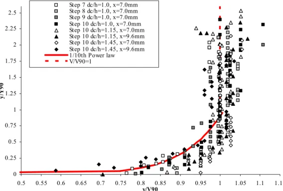
For all flow rates the velocity distributions had the same patterns. The velocity profiles compared well with a power-law function for y/Y90 < 1. For greater values of y/Y90 the velocity distributions tended

to be quasi-uniform. That is:

N / 1 90 90

Y

y

V

V

⎟⎟

⎠

⎞

⎜⎜

⎝

⎛

=

1

Y

y

0

<

≤

1

V

V

=

2

.

7

Y

y

1

≤

≤

Eq. (3-7) and (3-8) are shown in Figure 3.9.

The quasi-uniform profile of the velocity distribution for y/Y90 ≥1 is clearly visible in Figure 3.9. This

is confirmed by the values of V90 measured at each step edges for dc/h=1.33. V90/Vc as a function of

x/dc tends to remain constant (Figure 3.10). In the upper flow region (y=Y90), the flow structure

consisted predominantly of individual water droplets and packets surrounded by air. The present finding tended to suggest that most droplets were in a free-fall trajectory.

0 0.25 0.5 0.75 1 1.25 1.5 1.75 2 2.25 2.5 0.5 0.55 0.6 0.65 0.7 0.75 0.8 0.85 0.9 0.95 1 1.05 1.1 1.15 v/V90 y/ Y 90 Step 7 dc/h=1.0, x=7.0mm Step 8 dc/h=1.0, x=7.0mm Step 9 dc/h=1.0, x=7.0mm Step 10 dc/h=1.0, x=7.0mm Step 10 dc/h=1.15, x=7.0mm Step 10 dc/h=1.15, x=9.6mm Step 10 dc/h=1.45, x=7.0mm Step 10 dc/h=1.45, x=9.6mm 1/10th Power law V/V90=1

Figure 3.9 – V/V90 as a function of y/Y90 Flow rates: dc/h=1.15, dc/h=1.33, dc/h=1.45

Instrumentation: double-tip probes [Ø=0.25 mm, ∆x=7mm and ∆x=9.6 mm, ∆z=1.4 mm].

0 1 2 3 4 5 0 5 10 _x/dc 15 20 V 90/ V c V90/Vc dc/h=1.33, x=7 mm V90/Vc dc/h=1.15, x=7 mm V90/Vc dc/h=1.45, x=7 mm V90/Vc dc/h=1.15, x=9.6 mm V90/Vc dc/h=1.45, x=9.6 mm

Figure 3.10 –V90/Vc as a function of x/dc Flow rates: dc/h=1.15, dc/h=1.33, dc/h=1.45

Instrumentation: double-tip probes [Ø=0.25 mm, ∆x=7mm and ∆x=9.6 mm].

Experimental results included further the turbulence intensity Tu=u’/V where u’ is the root mean square of longitudinal component of turbulent velocity and V is the velocity. Tu could provide some information on the turbulence level in the flow. In Figure 3.11, Tu is shown as a function of y/Y90. The

similar trend to the bubble count rate in relation to y/Y90 (Figure 3.12). It is believed that high levels of

turbulence extending from y=0 to y=Y90 were caused by the strong aeration. Therefore turbulence

intensity distribution is strongly related to the bubble count rate distribution.

0 0.5 1 1.5 2 2.5 0 0.5 1 Tu 1.5 2 2.5 y/ Y 90 Step 7 dc/h=1.33 x=7mm Step 8 dc/h=1.33 x=7mm Step 9 dc/h=1.33 x=7mm Step 10 dc/h=1.33 x=7mm Step 10 dc/h=1.15, x=7mm Step 10 dc/h=1.15,x=9.6mm Step 10 dc/h=1.45, x=7mm Step 10 dc/h=1.45,x=9.6mm

Figure 3.11 – Tu as a function of y/Y90 Flow rates: dc/h=1.15, dc/h=1.33, dc/h=1.45

Instrumentation: double-tip probes [Ø=0.25 mm, ∆x=7mm and ∆x=9.6 mm, ∆z=1.4 mm].

0 0.5 1 1.5 2 2.5 3 0 5 10 15 20 25 30 F*dc/Vc y/ Y 90 0 0.5 1 Tu 1.5 2 2.5 F*dc/Vc Step 10 dc/h=1.33, x=7mm F*dc/Vc Step 10 dc/h=1.15, x=7mm F*dc/Vc Step 10 dc/h=1.45, x=7mm T u Step 10 dc/h=1.33 x=7mm T u Step 10 dc/h=1.15, x=7mm T u Step 10 dc/h=1.45, x=7mm

Figure 3.12 – Tu and F·dc/Vc as functions of y/Y90 Flow rates: dc/h=1.15, dc/h=1.33, dc/h=1.45

The relationship between the turbulence intensity and the bubble count rate is shown in Figure 3.13 as well as the correlation developed by CHANSON and TOOMBES (2002). That is:

1.5 c u c

F d

T

0.25 k

V

⎛

⋅

⎞

=

_{+ ⎜}

_⎟

⎝

⎠

where k is a constant of proportionality which is a function of the step geometry and flow rate. Note in Figure 3.14, Tumax increases linearly with x/dc and it is consistent with the trend of Fmax·dc/Vc. (Figure

3.8) 0 1 2 0 5 10 15 20 25 30 35 F*dc/Vc Tu T u Step 10 dc/h=1.33, x=7mm T u Step 10 dc/h=1.15, x=7mm T u Step 10 dc/h=1.45, x=7mm Correlation CHANSON and T OOMBES (2002)

Figure 3.13– Tu as function of F·dc/Vc. Flow rates: dc/h=1.15, dc/h=1.33, dc/h=1.45.

Instrumentation: double-tip probes [Ø=0.25 mm, ∆x=7mm and ∆x=9.6 mm, ∆z=1.4 mm].

0 1 2 0 2 4 6 8 x/dc 10 12 14 16 18 20 Tu m ax 0 5 10 15 20 25 F m ax*d c/ V c Tumax dc/h=1.33, x=7 mm Fmax*dc/Vc dc/h=1.33

Figure 3.14 – Tumax and F·dc/Vc as function of x/dc. Flow rate: dc/h=1.33.

3.2.3 Flow resistance

Skimming flows over stepped chute are characterized by significant form losses. Recirculating vortices develop between the main stream and the steps corners. Form drag and cavity recirculation are predominant and the form losses cannot be modelled by a Gauckler-Manning or Darcy-Weisbach formula. This is because two important hypotheses were neglected: the flow is not one-dimensional, it is not gradually varied. Nevertheless this study presents the flow resistance data in terms of an equivalent Darcy factor f because is a dimensionless shear stress that derives from the momentum equation.

In uniform equilibrium flows, the momentum principle states that the boundary friction force equals the gravity force component in the flow direction (HENDERSON 1966, CHANSON 2001, 2004). It yields:

0

P

g A sin

τ ⋅

= ρ ⋅ ⋅

⋅

θ

τ0 is the average shear stress between the skimming flow and recirculating fluid underneath

Pw is the wetted perimeter

ρw is the water density

g is the gravity constant

Aw is the water flow cross-section area

θ is the angle between the pseudo-bottom formed by the step edges and the horizontal.

In dimensionless terms and for a wide channel, Equation (3-10) becomes:

90 y Y y 0 0 e 2 2 w w w 8 g (1 C)dy sin 8 f U U = = ⎛ ⎞ ⋅ ⋅⎜_⎜ − ⎟_⎟ θ ⋅ τ _{⎝ ⎠} = = ρ ⋅

∫

fe is the Darcy friction factor for air-water flow

C is the local void fraction

y is measured normal to the pseudo-invert formed by the step edges Y90 is the distance normal to the pseudo-bottom where C=90%

Uw is equivalent clear-water flow velocity [m/s]

90 w w w Y 0 q q U d (1 C)dy = = −

∫

qw is water discharge per unit width

d is characteristic depth [m]

90 Y

0

d=

∫

In the present study, uniform equilibrium conditions were not achieved at the downstream end of the experimental channel. The equivalent Darcy friction factor fe was calculated using the differential form

90 y Y f y 0 0 e 2 2 w w w 8g (1 C)dy S 8 f U U = = ⎛ ⎞ − ⎜ ⎟ ⎜ ⎟ ⋅ τ _{⎝ ⎠} = = ρ

∫

Sf is the friction slope calculated as Sf= -δH/δx

H is the mean total head

x is the coordinate along the flow direction.

The friction factor data are shown in Table 3.4 and in Figure 3.15 as a function of ks=h*cosθ/DH where

DH is the hydraulic diameter. fe is related to the air-water flow properties and it was calculated

downstream the inception point for each discharge. Equation 3-13 presents, in dimensionless terms, the simplified analytical model of the pseudo-boundary shear stress used to compare flow resistance data. It was developed by CHANSON (2001).

d

2

1

f

K

=

⋅

π

fd is an equivalent Darcy friction factor estimate of the form drag

1/K is the dimensionless expansion rate of the shear layer. It is assumed to be a constant in a Prandtl mixing length model (RAJARATNAM 1976, SCHLICHTING 1979). For K=6 fd ≈0.2. The equivalent

friction factor ranged between 0.1 and 0.2 (Table 3.4, Figure 3.15).

Flow rate [dc/h] Discharge qw [m2/s] Re fe h*cosθ/DH 1.0 0.095 3.8E+05 0.220 0.63 1.15 0.116 4.6E+05 0.142 0.60 1.33 0.143 5.7E+05 0.167 0.50 1.45 0.161 6.4E+05 0.133 0.49 1.57 0.180 7.2E+05 0.158 0.43

h*cosθ/DH f, f e 0,3 0,4 0,5 0,6 0,7 0,8 0,9 1 0,1 0,2 0,3 0,4 0,5 fe f (CHANSON 01)

Figure 3.15 – Equivalent Darcy friction factor in air-water skimming flow and Eq. (3-13).

The values of the friction factor for stepped chutes are much greater than the values achieved on smooth concrete chute which typically are f=0.01 to f=0.03 (e.g. HENDERSON 1966, CHANSON 2004). Greater values of friction factor mean larger energy dissipation taking place along a stepped chute compared with a smooth chute.

The present data are consistent with the previous studies conducted for stepped chute with same step height (h=0.10[m], θ=22°) and similar discharges (Table 3.5).

CHANSON et al. (2002) investigated the flow resistance in skimming flow based upon experiments with channel slopes ranging from 5.7° to 55°. The data were compared with a reanalysis of several past studies where the slopes were between 15.9° and 59°, h > 0.020 m and Re>105_{. The stepped}

chutes were classified by the slopes: flat chutes (θ < 20° ) and steep chutes (θ > 20°). On steep chutes the friction factor was ranging from 0.105 up to 0.30. Present experimental results achieved the same range.

Table 3.5 – Flow resistance in stepped chute θ=22°. Reference Qw [m3/s] fe 0.164 0.133 0.182 0.10 0.2005 0.12 GONZALEZ and CHANSON (2004)

0.2195 0.15 0.182 0.143 0.164 0.157 0.147 0.196 0.130 0.184 0.124 0.215 0.114 0.283 0.103 0.157 TOOMBES and CHANSON (2001)