Department of Engineering
Doctorate in Engineering and Chemical
of Materials and Constructions
(XXX cycle)
“Experimental tests and Numerical analysis
for an Air Cavity Yacht”
PhD Candidate: Dott. Ing. Felice Sfravara Tutor: Prof. Ing. Vincenzo Crupi Coordinator: Prof. Signorino Galvagno
2. Introduction ... 2
2.1 Background and motivation ... 2
2.2 Objectives and principal points of the research ... 3
2.3 Outline of the thesis ... 3
3. Literature Overview ... 4
3.1 The towing tank test ... 4
3.2 Evolution of analytical and numerical approach ... 5
3.3 Air Cavity technology ... 8
4. Background Theory ... 9
5. Experimental tests ... 12
5.1 Method for towing tank tests ... 12
5.2 Design and shape of all models tested ... 14
5.3 Model manufacturing ... 32
5.4 Results and Discussion of experimental Tests ... 38
6. Computational Fluid Dynamics simulations ... 51
6.1 CFD Method ... 51
6.2 CFD results and comparison with experimental tests – Model B ... 59
6.3 CFD results and comparison with experimental tests – Model C ... 73
7. Conclusions ... 87
________________________________________________________________________________
Felice Sfravara 1
1. Nomenclature
Definition Symbol Formula Unit
Overall Length LOA - m
Waterline Length LWL - m
Projected Chine Length LP - m
Waterline Beam BWL - m
Wetted Surface S m2
Longitudinal Position of Buoyancy LCB m
Longitudinal Position of Floating Centre
LCF m
Vertical Position of Buoyancy VCB m
Wetted Surface SW m2
Area to Water Line AWL m2
Transversal Metacentric Height KMt m
Sectional Area to displacement A
Longitudinal Metacentric Height KMl m
Centimeter Trim Moment Mu t*m/cm
Centimeter Displacement Δu t/cm
Projected Maximum Beam BPX - m
Projected Beam at generic X position
BPC - m
Projected Beam Transom BPT - m
Projected Medium Beam BPA 𝐴𝑃
𝐿𝑃
m
Deadrise Angle β - °
Height of medium buttock line HLM - m
Draft T - m
Displacement Mass Δ - t
Displacement Volume
Longitudinal center of gravity xG - m
Projected Area AP - m2 Velocity of Ship VS - m/s Velocity of Model VM - m/s Froude number Fn - Length of Ship LS - m Length of Model LM - m Scale λ 𝐿𝑆 𝐿𝑀 - Number of Steps NST - -
Position of the step relative to the transom
LST - m
Area Step SST - m2
________________________________________________________________________________
Felice Sfravara 2
Dimensions - Basis x Height BIN x HIN
- m x m
Area of nozzles SIN - m2
Dimensions - Basis x Height Rails BR x HR - m x m
Transversal Distance Between Rails
TDR - m
Number of rails NR - -
Volumetric Flow Rate Q m3/s
Flow rate Coefficient CQ 𝑄
𝑆𝐼𝑁𝑉𝑀
-
2. Introduction
Abstract
This chapter introduce the reader in the principal motivations of this research. There are also explained the principal objectives of the thesis with the methodologies used in order to reach the results obtained. A brief outline of the thesis with a brief explanation of each chapter.
2.1 Background and motivation
Each moving object in the earth or the principal industrial processes or simply the daily activities of humans involve the use of some kind of fluids. This interaction can be advantageous or disadvantageous. The deep knowledge of the main features of fluid flow allows to manage it with great advantages in terms of efficiency and sustainability, principally when the problem is the reduction of the resistance during the movement of a body.
In the case of naval engineering, there is a strong interaction between the fluid and the ship. This interaction leads to a different effects, the most important one is the resistance during the navigation. The resistance of a ship is composed by two principal components: frictional resistance and wave resistance. Both of them must be reduced in order to keep the resistance low. The wave component is strongly dependent by the shape of the hull, so in preliminary phase, is possible to find, with different techniques, the better shape for reducing it. More complex is the reduction of the frictional component, because it depends on the contact between the surface of the ship and the water.
The most difficult problem is the reduction of this component with methodologies applicable on the ships. There are many examples of drag reduction on flat plate, for example application of particular coatings or particular geometry but these passive methods are not suitable for the application on the ship.
Another way is the injection of the air under the hull, this condition allows to separate the surface of the ship from the water. There are many examples of application of this method on flat plate
________________________________________________________________________________
Felice Sfravara 3
models or on displacement hulls. This method seems the most promising one. These studies show that the injection of the air with a stable layer of air allows to reduce the frictional resistance. This work was partially supported by European Union funding. The principal aspect of this work is the application of the air cavity on a high speed ship in model scale and real scale.
2.2 Objectives and principal points of the research
Thanks to many studies in literature is possible to know that the air injection under a stepped flat plate or under scale model of ship leads to a reduction of frictional resistance. There are also new applications on real scale ship. This technology is also under study and it is not widely used yet. Objective of the research is to improve the knowledge of air-cavity phenomena with a systematic study on different design bottom hull solution for the same type of planing hull. The approach is oriented to find the better design solution for the application of air-cavity on a yacht of 18 meters. Four different scale models have been tested to different velocities and air flow.
The second part of the thesis involves the validation of computational fluid dynamics method for this kind of problem and so to quantify the potentiality of the CFD for solving this complex phenomena under the hull. The method used is the URanse (Unsteady Reynolds Navier Stokes method). The results could be used for modifying the hull geometry in order to better accommodate the air layer.
2.3 Outline of the thesis
The literature overview chapter introduces the reader to the literature of the two principal techniques for solving the problem of resistance prediction in naval engineering, the experimental methods and the numerical approach. A review of the history of the air cavity is proposed in this chapter with particular focus on the experimental and numerical approaches.
The Nomenclature chapter helps the reader to understand the meaning of different symbols inside the thesis.
Background theory chapter introduces the reader to the principal equation to the basis of the fluid dynamic flow, with the derivation of the Navier Stokes Equations. A brief review of the principal hypothesis is reported in this chapter with the principal boundary conditions used in naval field in order to solve the problem of the flow around the hull.
Experimental tests is the chapter that concerns the description of the experimental part of this research. A brief review of the ITTC method in the towing tank tests is shown with particular interest on the Froude’ Law. In the second sub-chapter the reader find a detailed description of all hull shapes used for the experimental tests, with general and specific dimensions. The third sub-chapter analyses the construction making phase with a detailed explanation of the all tests performed in the towing tank of Naple. The last sub-chapter concerns a review of all results and discussion about the use of air cavity in this kind of hulls.
________________________________________________________________________________
Felice Sfravara 4
Computational Fluid Dynamic is the chapter that concerns the use of the numerical approach for solving this kind of problem. A first part explains the general approach used by all commercial software. A step-by-step explanation of all settings is reported with the CFD method with all parameters about mesh and solver controls. The method is developed in order to find the better settings for air injection condition and an uncertainty analysis is proposed during the numerical simulations. In order to test the method, another case study is proposed.
The last chapter concerns a resume of principal aspects of the thesis and the main results obtained during the three years of doctorate.
3. Literature Overview
AbstractThis chapter introduce the reader in the state of art of the towing tank tests, the state of art of evolution of numerical approach and the last development of the air cavity technology.
3.1 The towing tank test
Since 1452 Leonardo da Vinci carried out tests on different models of ships for resistance prediction. In his work, three ships with the same general dimensions but with different aft-and-fore shapes have been tested (Tursini, 1953). The interest on this problem pushed other researchers to find solutions for defining new experimental methods. The first approach was to build woven models towed by falling weights inside a tank (Baker, 1937). Todd proposed a paper with a general methodology for experimental tests in the 1951 (Todd, 1951). In all these experiments the real problem was to scale the results from the model scale to full scale. The solution to this problem has been proposed by Froude, his idea was to divide the total resistance in two different independent components: frictional and wave (Froude, 1955). The literal words of Froude were “The (residuary) resistance of geometrically similar ships is in the ratio of the cube of their linear dimensions if their speeds are in the ratio of the square roots of their linear dimensions”. The residuary component cited by Froude is the total resistance minus the resistance of an equivalent flat plate with the same wetted area and length and moving with the same velocity of the hull (at model and full scale). The idea was to divide the total resistance in the part produced by the viscous effects between the hull surface and the water, the other part produced by the waves. Froude made his first experimental tests with falling weights method but he was not satisfied because of the limitations of this technique. Successively, Froude proposed a new towing tank with the use of a mechanical propelled carriage system for towing the model in a tank. The friction component was obtained with experimental tests on equivalent flat plate at model and full scale or with a formula proposed by Froude. This component was subtracted to the total component of the resistance at model scale and the result was the residuary component of resistance at model scale. Thanks to Froude law, the residuary component was scaled in full scale and added to the frictional equivalent flat plate component so obtaining the total resistance to full scale. The two mains specifications in order to apply this method were: the model scale and the full scale must be with the same shapes (geometric similitude) and the ratio between the velocities must be in ratio of the square roots of their linear dimensions. The frictional formula proposed by Froude was independent by an important number:
________________________________________________________________________________
Felice Sfravara 5
Reynolds number. From the 1927 until to 2006 different formula for the frictional component of resistance have been proposed (Lazauskas, 2005). The first researcher introduced a new formula in towing tank test was Schoenherr but only in 1957 the International Towing Tank Conference introduced the new procedure (ITTC, 1957). In this procedure the viscous effects were defined by a single formula without considering the effects of the 3-D shape of the hull. The ITTC introduced another extrapolation technique in order to take in account this particular effects (International Towing Tank Conference, 1978). All the towing tank use the ITTC’57 or ITT’78 method, both of these methods are based on a law very old but reliable and useful for resistance prediction. The method during the years is changed respect to the formula used for solving the friction component of the resistance in order to take in account the scale effects and the great difference between the Reynolds number at model scale and at full scale. In this research all experimental tests have been conducted in Towing tank of Naple with the ITTC’57 methodology (principally used for high speed hull).
3.2 Evolution of analytical and numerical approach
From the beginning of the use of numerical and analytical methods, the idea was to solve the problem of total resistance prediction with the separation of this quantity in two independent components: free-surface and wave component and frictional component.
Before the advent of modern computer with great power capacity, the solution of fluid flow around the ship were based on analytical methods. All these methods were based on a simplification: the inviscid flow condition, the viscous effects were neglected. The first result presented in literature with an analytical method for solving the resistance problem was proposed by Michell (Michell, 1898). In this case, the ship had a slender shape and the viscosity of the fluid was neglected. All the boundary conditions were linearized and the boundary condition relative to hull surface was defined along the centre line. Michell found a mathematical expression for the pressure distribution around the ship. The integration of this quantity along the hull allowed to know the pressure resistance. In the 1951, Havelock proposed for the first time the use of the energy concept (Havelock, 1951). The wave resistance was measured thanks to this energy, the novelty of the approach was the use of sources and sinks elements. These elements were respectively emitter and absorber of energy. The sources were positioned along the centre line and the intensity of energy was dependent by the position and the local angle of the waterline. Thanks to the sum of the sources effects the wave resistance could be determined. The first idea of optimization of hull shape was proposed by Inui (Inui, 1980), the optimization concerned the wave component of resistance, also in this case the viscous effects were neglected. In the same period the same author proposed a study in order to quantify the non linear effects of the free-surface on the wave resistance (Inui and Kajitani, 1977). Thanks to the introduction of the computers and with the increase of the computational power many different methods have been developed during the last years based on numerical techniques. The first improvement respect the analytical methods was to define a hull surface with quadrilateral elements called panels and the possibility to apply the boundary condition of the hull on these quadrilateral elements respecting the 3D shape of the hull. The method is known as panel method and the application of this method in fluid dynamics was explained by Hess (Hess, 1990). At first,
________________________________________________________________________________
Felice Sfravara 6
the panel method was used in aerodynamic problems but with the idea proposed by Dawson (Dawson, 1977) also in naval problems this method became useful. Dawson solved the problem of the flow around the ship applying the panel method both for the hull surface and for the free-surface. The limitation was that Dawson applied linearized boundary conditions for the free-free-surface. A refinement of the Dawson approach with a real free surface boundary condition was successively developed by Janson (Carl-Erik Janson, 1997).
During this years, researchers exploring also methods for solving the other component of resistance, the frictional one. The problem was to solve the boundary layer near the hull surface. Also in this case, the help of the computational power is very important. In the 1968, the first solution for the boundary layer around a 2D object was presented by Kline et al. (Kline et al., 1968) . The great problem of these models was the prediction of the flow around the stern of the ship, principally in the flow separation zones. Larsson (Larsson et al., 1990) during the workshop in Gothenburg, described all methods and focused the attention on the necessity to solve this problem with new methods. These new methods should be able to solve simultaneously the boundary layer problem and the free-surface conditions.
The most promising one was the Reynolds-Averaged Navier stokes method (RANS). The RANS method (successively explained) allows to remove the fluctuations of the velocity components produced by the turbulence and reduce the problem of turbulence with an artificial modelling of the Reynolds stresses components (six unknown components). The researchers focused on three different key elements in order to solve with computational approach the RANS equations: the grid generation, the algorithm development and the turbulence modeling. The last one was the most important one because it involves the use of a mathematical model in order to approximate a physical behavior. The great effort of all researchers was to find the better model of turbulence for each industrial case. This assumption is important because a single turbulence model is not sufficient for all industrial cases. A great explanation of all turbulence models have been proposed by Wilcox (Wilcox, 2006).
The great potentiality of RANS methods have been discussed during other different workshops (Kodama et al., 1994) and the increase of the computer power allowed to increase the efficiency of this method, principally for solving the full-scale viscous flow with the free-surface problem. A grid-dependence study of the RANS method with a computational grid regenerated to follow the free surface condition has been proposed by Hino (Hino, 1994). The numerical approach concerned the use of three different grids with different elements density. The solutions have been compared with each other and with experimental data and the grid dependence of these solution has been discussed. The hull under investigation was a Series 60. Another study proposed by the same author concerned the influence of the turbulence models on the final results (Hino, 1995). The author used two different one-equation turbulence models for the prediction of the resistance of two tankers (HSVA Tanker and the Dyne Tanker). The results were in great accordance with the experimental results. The author used the one-equation turbulence model approach, but with the increase of the computer power other different turbulence methods have been developed.
________________________________________________________________________________
Felice Sfravara 7
A great international workshop has been organized in Gothenburg in 2000 (Larsson et al., 2003). The principal theme of the workshop was the application of computational fluid dynamics in solving the ship flow. The principal objectives of the workshop were understanding the better solution for the turbulence modeling and the capacity of wave prediction also away from the hull with this new numerical method. The results were very important because with this new approach the flow around the stern was appropriately computed, the full-scale viscous flow may be computed without problem and the wave prediction near and away from the hull was predicted accurately. In the end of the workshop, an important concept has been recommended: the necessity of an uncertainty analysis during the process of verification and validation of the numerical approach.
In the last years, the application of numerical methods for the resistance prediction is widely used in ship design, principally for problems of optimization shape in order to reduce the total drag. Techniques that use the URANSe (the Unsteady application of the RANS methods) are applied to avoid the towing tank tests and speed up the optimization process. A typical study is the hydrodynamic hull shape optimization as reported by Wilson et al. (Wilson et al., 2010) for standard ship or the prediction of drag of new type of ships such as catamarans (He et al., 2013). An important aspect is the simulation of the interaction between fluid and rigid body motion of the ship or any floating object. In the first case a typical example is the calculation of the trim and sinkage (Formaggia et al., 2008), in the second case typical examples are the study of offshore wind turbine (Quallen and Xing, 2016) or system such as wave energy converter (Brusca et al., 2015). In case of large deformation caused by fluid-dynamics pressure or forces the use of rigid body motion is not adequate, so new methodologies with the use of direct coupling between mechanical and fluid-dynamics solvers can be used. In this sense, analysis of shape deformation of parachute is a typical example (Takizawa et al., 2015) or the shape deformation of sails (Cella et al., 2017). The URANSe method has a great approximation: the turbulence is solved with a model. In the last years, a new techniques allows to solve the all scales of the turbulence eddies directly, without approximation. This technique is called Direct Numerical Simulation (DNS) and involves a great requests of computational power, a brief review of this technique has been reported by Moin and Mahesh (Moin and Mahesh, 1998). The direct numerical simulation is used in order to solve problem of wall turbulence in a channel flow (Myoungkyu and Moser, 2015) or usually it is used for solving problem of transport of solid particle caused by an incompressible flow (Kidanemariam and Uhlmann, 2014). In the field of naval ship, this technique is still avoided because the domain is too big and the time solution could be too much expansive. In new computational fluid dynamic software there is a new approach: Large Eddy Simulation (LES). It is a good compromise between the URANSe method and the DNS one. In this case part of the scale of the turbulence eddies is solved in a direct way (naturally with specific conditions in the sizing of the mesh) and part of these eddies are solved with the classic turbulence models. This technique is under investigation and the principal challenges have been described by Fureby (Fureby, 2016). An interesting application of the LES method is the cavitation. In this phenomena is interesting to understand the cavitation structures and the influence of the turbulence on these structures. An application of the LES for cavitation problems of a hydrofoil is proposed by Ji et al (Ji et al., 2015). The same technique is applied by Balaras et al. (Balaras et al., 2015) for solving the problem of cavitation around a submarine propeller, the technique allows to solve the tip vortices of the propeller in open water condition. Also in this case, the time of
________________________________________________________________________________
Felice Sfravara 8
simulation is increased respect to the URANSe solution but it could be a good compromise in cases where the study of turbulence eddies is very important.
3.3 Air Cavity technology
The initial theoretical modeling for air cavities under plate have been developed by Butuzov (Butuzov, 1968). This idea was transferred to ships with a full-scale trials of a boat with an air cavity (Butuzov et al., 1988). An alternative to the air-cavity is the microbubbles method. The pioneer in this field were McCormick and Bhattacharyya (McCormick and Bhattacharyya, 1973). Successively Kodama proposed an experimental test with circulating water tunnel (Kodama et al., 2002). An interesting device in combination with the use of micro-bubbles application is proposed by Kumagai et al. (Kumagai et al., 2015). A low pressure zone is produced rear a hydrofoil and the injection of the micro-bubbles is conducted in this zone taking in advantage the optimal environmental condition produced by the device. Merkle and Deutsch highlighted that the microbubbles method is ineffective for low velocity range (Merkle and Deutsch, 1989) and Ferrante and Elghobashi showed that, with the increase of Reynolds number, the reduction of frictional resistance decreased (Ferrante and Elghobashi, 2004). The disadvantages of the technology with microbubble, showed by authors, pushed the studies in the direction of air-cavity. A brief review of all technologies for friction drag reduction is proposed by Ahmadzadehtalatapeh and Mousavi (Ahmadzadehtalatapeh and Mousavi, 2016). Ceccio (Ceccio, 2010) proposed different applications and a detailed explanation of the distribution of the air under the hull during the injection. The economic saving is another aspect to take in account, a brief examination is reported by Mäkiharju et al. (Mäkiharju et al., 2012). Many authors studied the principal characteristics of the cavity in various conditions, experimental and numerical tests have been conducted in various forms and a brief review is proposed here. Matveev shown the principal parameters that influence the cavity of air (Matveev, 2003) with a numerical study for the simplified configuration of a rear-ward-facing step on the lower surface of horizontal wall for choosing the correct position of propulsion and lifting devices. Another important study was about the interaction between waves and cavity, it was solved with a numerical simplified approach by Matveev (Matveev, 2007). A study of air-ventilated cavities under a simplified hull has been undertaken by Matveev (Matveev, 2012), experiment with a 56-cm-long stepped-hull model were carried in an open-surface water channel at flow velocities of 28-86 cm/s. Following the report on flat plate case with air cavity proposed in the Emerson Cavitation Tunnel of Newcastle University by Slyozkin (Slyozkin et al., 2014), Butterworth et al. proposed an experimental test on an existing container ship model with a middle section of 2.2 m (Butterworth et al., 2015) and a 0.43 x 0.09 m2 area for air cavity. The model experiments produced results ranging from 4% to 16% drag reduction. Always on the flat plate, application of submerged superhydrophobic (SHPo) surface is proposed by Lee et al. (Lee et al., 2016) with an entrapped gas called plastron, the application is suitable for laminar flow. Jang et al. (Jang et al., 2014) conducted experimental tests on the flat plate and successively on the model with also a self-propulsion test equipped with air lubrication system. Amromin (Amromin, 2016) reported an analysis of the interaction between the air cavity and the boundary layer. The scale factor of the air layer drag reduction has to be take in account. Indeed this effect could change significantly the results when they are transferred directly to full scale model. In this terms, an investigation of the scaling factor is reported by Elbing et al.
________________________________________________________________________________
Felice Sfravara 9
(Elbing et al., 2013). There is a great interest also in the shipyard industries for this technology, Mitsubishi Heavy Industries developed an air lubrication system and carried out tests in order to verify the efficiency in terms of frictional resistance reduction (Mizokami et al., 2013). There are less experiment tests for planing hulls; an important example is proposed by Matveev (Matveev, 2015) where there is a numerical method for prediction of drag reduction validated with experimental data. The same author developed a platform, with the necessary instruments, for testing different typologies of Air Cavity Ships (ACS) in order to improve and optimize this kind of technology (Matveev et al., 2015). An experimental work with analysis of the total resistance, trim, sinkage and wave pattern for high speed craft with artificial air cavity is proposed by Gokcay et al. (Gokcay et al., 2004). The experimental data are not only important for better understanding the artificial air cavity phenomena but also in order to validate, in this kind of problem, the URANSe (Unsteady Reynolds-Averaged Navier Stokes equation) methods. In the case of ACS, the problem is the multiphase flow with different scales interaction, the big one that concerns the waves’ free surface and the small one that concerns the free surface of cavity (Cucinotta et al., 2017a, 2017b).
In the case of ACS, the problem is the multiphase flow with different scales interaction, the big one that concerns the waves’ free surface and the small one that concerns the free surface of cavity (Cucinotta et al., 2017a, 2017b). An initial approach with commercial software is reported by Maimun et al. (Maimun et al., 2016).
4. Background Theory
AbstractThis chapter is about the theory of fluid-dynamic around a ship. The first part concerns the principal physical conditions in order to obtain the Navier Stokes equations. There is a complete description of the boundary conditions and the main assumptions for solving this complex phenomena.
The first objective of a naval architect engineer is to know, in preliminary phase, the resistance of the ship during the navigation to a specified velocity condition. In order to obtain this quantity, the engineer must know the physic principle of the fluid dynamics around the ship.
The start point of each consideration are two simple physical concepts applied to an infinitesimal incompressible fluid element: the conservation of mass and the Newton’s second law. Inside an infinitesimal element the total net transport of mass out of element have to be zero in absence of sources inside the element (Eq. 4.1 – Continuity Equation).
𝜕𝑢 𝜕𝑥+ 𝜕𝑣 𝜕𝑦+ 𝜕𝑤 𝜕𝑧 = 0 (4.1) The Newton’s second law starts with a simple equation:
________________________________________________________________________________
Felice Sfravara 10
A physical consideration is that in a fluid mechanic problem three different types of forces must be considered: body forces 𝑑𝐹⃗⃗⃗⃗⃗⃗⃗ , viscous forces 𝑑𝐹𝑏 ⃗⃗⃗⃗⃗⃗ and pressure forces 𝑑𝐹𝑣 ⃗⃗⃗⃗⃗⃗ . 𝑝
Considering a coordinate system with the z-axis along the direction of the gravity, the only body force needs to be considered is the gravity force (Eq.4.3).
𝑑𝐹𝑏𝑧
𝑑𝑚 = −𝑔 (4.3)
The pressure forces depend by the gradient of the pressure along all directions inside the infinitesimal element (Eq. 4.4-4.5-4.6).
𝑑𝐹𝑝𝑥 𝑑𝑚 = − 1 𝜌 𝜕𝑝 𝜕𝑥 (4.4) 𝑑𝐹𝑝𝑦 𝑑𝑚 = − 1 𝜌 𝜕𝑝 𝜕𝑦 (4.5) 𝑑𝐹𝑝𝑧 𝑑𝑚 = − 1 𝜌 𝜕𝑝 𝜕𝑧 (4.6) The viscous forces depend by the stresses inside the infinitesimal element, there are tangential viscous stresses and normal viscous stresses. The sum of each component of stress along respectively x-y-z direction defines the total viscous force along that direction (Eq. 4.7-4.8-4.9).
𝑑𝐹𝑣𝑥 𝑑𝑚 = 1 𝜌[ 𝜕𝜎𝑥𝑥 𝜕𝑥 + 𝜕𝜎𝑦𝑥 𝜕𝑦 + 𝜕𝜎𝑧𝑥 𝜕𝑧 ] (4.7) 𝑑𝐹𝑣𝑦 𝑑𝑚 = 1 𝜌 [ 𝜕𝜎𝑥𝑦 𝜕𝑥 + 𝜕𝜎𝑦𝑦 𝜕𝑦 + 𝜕𝜎𝑧𝑦 𝜕𝑧 ] (4.8) 𝑑𝐹𝑣𝑧 𝑑𝑚 = 1 𝜌 [ 𝜕𝜎𝑥𝑧 𝜕𝑥 + 𝜕𝜎𝑦𝑧 𝜕𝑦 + 𝜕𝜎𝑧𝑧 𝜕𝑧 ] (4.9)
The great hypothesis to the base of the Navier Stokes equation is the one defined by Newton. The stress components 𝜎𝑖𝑗 are proportional to the rate of strain tensor (Eq. 4.10) with constant of proportionality the dynamic viscosity µ (Eq. 4.11). This correlation allows to define the stress components in function of the velocities.
𝑆𝑖𝑗 = 𝜕𝑢𝑖 𝜕𝑥𝑗+
𝜕𝑢𝑗
𝜕𝑥𝑖 (4.10) 𝜎𝑖𝑗 = µ 𝑆𝑖𝑗 (4.11)
All these considerations lead to the Navier Stokes equations, a second order nonlinear system of differential equations (Eq. 4.12-4.13-4.14) and the continuity equation (Eq. 4.15). The entire system is a set of four equations that together constitute a closed system for the four unknown variables: Pressure (p), vector velocity (u,v,w).
________________________________________________________________________________ Felice Sfravara 11 𝜕𝑢 𝜕𝑡 + 𝑢 𝜕𝑢 𝜕𝑥+ 𝑣 𝜕𝑢 𝜕𝑦+ 𝑤 𝜕𝑢 𝜕𝑧= − 1 𝜌 𝜕𝑝 𝜕𝑥+ 𝜈 ( 𝜕2𝑢 𝜕𝑥2+ 𝜕2𝑢 𝜕𝑦2+ 𝜕2𝑢 𝜕𝑧2) (4.12) 𝜕𝑣 𝜕𝑡 + 𝑢 𝜕𝑣 𝜕𝑥+ 𝑣 𝜕𝑣 𝜕𝑦+ 𝑤 𝜕𝑣 𝜕𝑧 = − 1 𝜌 𝜕𝑝 𝜕𝑦+ 𝜈 ( 𝜕2𝑣 𝜕𝑥2+ 𝜕2𝑣 𝜕𝑦2+ 𝜕2𝑣 𝜕𝑧2) (4.13) 𝜕𝑤 𝜕𝑡 + 𝑢 𝜕𝑤 𝜕𝑥 + 𝑣 𝜕𝑤 𝜕𝑦 + 𝑤 𝜕𝑤 𝜕𝑧 = − 1 𝜌 𝜕𝑝 𝜕𝑧− 𝑔 + 𝜈 ( 𝜕2𝑤 𝜕𝑥2 + 𝜕2𝑤 𝜕𝑦2 + 𝜕2𝑤 𝜕𝑧2) (4.14) 𝜕𝑢 𝜕𝑥+ 𝜕𝑣 𝜕𝑦+ 𝜕𝑤 𝜕𝑧 = 0 (4.15)
The system of Navier Stokes equation is elliptical with partial differential equations, this means that each boundary in the domain must have an initial condition. The domain around the ship has different boundaries: the hull surface, the free surface and the domain far from the hull. For each of these boundaries a condition must be imposed.
On the hull surface, the so called no-slip condition have to be imposed. This condition is relative to the components of velocity:
𝑢 = 𝑣 = 𝑤 = 0
On the free surface, where there are two phases in contact, liquid and gas, two different boundary conditions have to be defined.
The first one is a dynamic condition that expressing that the two phases on this surface must have
the same velocities. This condition is imposed with the equality of the forces of the two phases. The equations 4.16-4.17 define the equality between the tangential components (s,t) for the water (w) and for the air (a).
𝜎(𝑛𝑠)𝑤=𝜎(𝑛𝑠)𝑎 (4.16) 𝜎(𝑛𝑡)𝑤=𝜎(𝑛𝑡)𝑎 (4.17)
In the case of the normal component (Eq. 4.18) of the force respect to the free surface, must be taken in account the effect of the surface tension (Δpγ).
(𝜎(𝑛𝑛)− 𝑝)𝑤 = (𝜎(𝑛𝑛)− 𝑝)𝑎+ 𝛥𝑝𝛾 (4.18)
The second one is a kinematic boundary that expressing the no flow through the surface. In this case
the condition is that the vertical component of the velocity w must be equal to the derivative of the wave height respect the time (Eq. 4.19)
𝑤 =𝑑𝜁
________________________________________________________________________________
Felice Sfravara 12
Another important condition is the one to infinity. The extension of the domain is not limited. All disturbances have to go zero far from the hull surface.
There are three principal ways to solve the problem of resistance prediction of ship: empirical methods, experimental methods and numerical methods. The work proposed in this research uses the experimental techniques in order to obtain the resistance of all models proposed. Thanks to results from these techniques a numerical approach has been investigated and validated for a model and successively used for other one.
5. Experimental tests
AbstractA first part of this chapter describes the method used for solving the problem of resistance prediction with the use of the towing tank. The second chapter explains the hull shapes tested and all the tests conducted in the towing tank. Third chapter puts the attention in the building part of the models and in the final chapter all results and discussion are presented.
5.1 Method for towing tank tests
If the variables inside the system of differential equations and in the boundary conditions are made dimensionless, the result is a system of differential equations governed by four dimensionless parameters: the Reynolds number (Rn), the Froude Number (Fn), the Weber (Wn) number and the Euler number (En). This transformation of the Navier-Stokes equations is explained by White (White, 2014).
The Reynolds number (Eq.5.1) is a parameter that allows to take in account the effects of the viscosity of the fluid. It is directly inside the equations of Navier Stokes. The Froude number (Eq.5.2) is a parameter that allows to take in account the effects of the gravity on the free surface, it appears inside the dynamic boundary condition on the free surface. The Weber number (Eq. 5.3) is a parameter that allows to take in account the surface tension effects, with particular interest on the spray and breaking waves. The Euler number (Eq.5.4) is a parameter that allows to take in account the effects of cavitation, this number is important only for cases where there is cavitation conditions. 𝑅𝑛 =𝑉𝐿 𝜈 𝐸𝑞. (5.1) 𝐹𝑛 = 𝑉 √𝑔𝐿 𝐸𝑞. (5.2) 𝑊𝑛 = 𝜌𝑈2𝐿 𝛾 𝐸𝑞. (5.3)
________________________________________________________________________________
Felice Sfravara 13
𝐸𝑛 = 𝑝𝑎
𝜌𝑈2 𝑒𝑞. (5.4)
The sufficient and necessary condition for flow similarity between geosim bodies (two bodies with the same shape) at different scales is the condition of constancy of these four parameters (Larsson and Raven, 2010). If the above parameters are unchanged between two geosim bodies, the solution in no dimensional form is unchanged.
Inside the towing tank, by definition, the model has a length smaller than that of the ship, in order to keep all parameters equal to real scale the model speed should be adjusted and it is not possible to keep the four parameters at the same time equal. For example, in order to keep the same Froude number the velocity of the model has to be smaller than of that of the full scale, contrarily for the consistence of the Reynolds number or Weber number the velocity has to be higher. Only one parameter at a time can be maintained equal to real scale and the other three have to be sacrificed. The Euler number concerns cavitation problems, usually in the flow around the hull no cavitation problem are found and it is possible to sacrifice this parameter. The Weber number governs the spray and the surface tension effects, they have a little effect on the total of resistance and this number can be sacrificed (Larsson and Raven, 2010). The choice is reduced between two parameters, the Reynold number and the Froude number.
Thanks to the studies of Froude (Froude, 1955), the approach for calculating the resistance of the ship in experimental way is based on an important concept: the possibility to split the resistance or the total coefficient of resistance (Eq. 5.5) in two independent parts governed by the Froude number (residuary part - CR) and the Reynolds number (frictional part CF).
𝐶𝑇 = 𝑅𝑇
1/2𝜌𝑆𝑉2 𝐸𝑞. (5.5) 𝐶𝑇 = 𝐶𝐹(𝑅𝑛) + 𝐶𝑅(𝐹𝑛) 𝐸𝑞. (5.6)
In the towing tank is conducted the test with a a geosim model to the same Froude number of the hull at full scale. In order to have the same Froude number, the velocities to model scale and full scale must be defined by the equation:
𝑉𝑀 = 𝑉𝑆√ 𝐿𝑀
𝐿𝑆 𝐸𝑞. (5.7)
The test in the towing tank allows to obtain the total resistance of the model and so the total coefficient of resistance CTM. The second step is to use the ITTC’57 formula in order to find the frictional component of the model (Eq.5.8). In this equation the number of Reynolds is the one in model scale.
𝐶𝐹𝑀 = 0.075
________________________________________________________________________________
Felice Sfravara 14
Considering that the residuary component of the model is equal to the one at full scale (Eq.5.9) and adding the frictional component, this time with the Reynolds number at full scale, the total coefficient at full scale is obtained (Eq.5.10).
𝐶𝑅𝑀 = 𝐶𝑇𝑀− 𝐶𝐹𝑀 = 𝐶𝑅𝑆 𝐸𝑞. (5.9) 𝐶𝑇𝑆 = 𝐶𝑅𝑆+ 0.075
(log 𝑅𝑛𝑆− 2)2 𝐸𝑞. (5.10)
5.2 Design and shape of all models tested
The starting point was the original hull form (Model A) without cavity. This hull form was relative to an Abacus Marine yacht which main dimensions and constructive characteristics are shown in Table 1. This model is used as a basis for the successively comparison with the models with different bottom shape. The hull design is shown in Figure 1 and all the hydrostatic characteristics are reported in Figure 2. The original hull is a typical planning hull with V shape.
Symbol Ship Model Unit
LOA 17.53 2.92 m LWL 14.88 2.48 m LP 16.20 2.70 m BWL 4.35 0.72 m BPX 3.72 0.62 m BPA 3.20 0.54 m BPT 3.66 0.61 m T 1.00 0.17 m Δ 34 0.15 t S 69 1.92 m2 AP 52.2 1.45 m2 xG (% of LOA) 35.18 % 35.18 % -
________________________________________________________________________________
Felice Sfravara 15
Figure 1 - Lines plan at full scale of Model A
Figure 2 - Hydrostatic quantities of Model A at full scale
0 1 2 3 4 5 6 7 8 9 10 11 12 13 14 15 16 17 0.1 0.3 0.5 0.7 0.9 1.1 1.3 1.5 0.1 0.2 0.3 0.4 0.5 0.6 0.7 0.8 0.9 1 1.1 1.2 1.3 1.4 1.5 0 5 10 15 20 25 30 35 40 45 50 55 60 65 70 75 80 85 90 Δ [t] Volume [m^3] AWL [m^2] S [m^2] KMl [m] LWL [m] BWL [m] LCB [m] VCB [m] LCF [m] KMt [m] Mu [t*m/cm] Δu [t/cm]
________________________________________________________________________________
Felice Sfravara 16
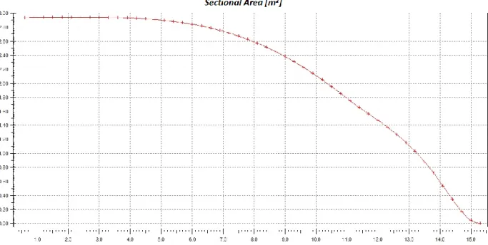
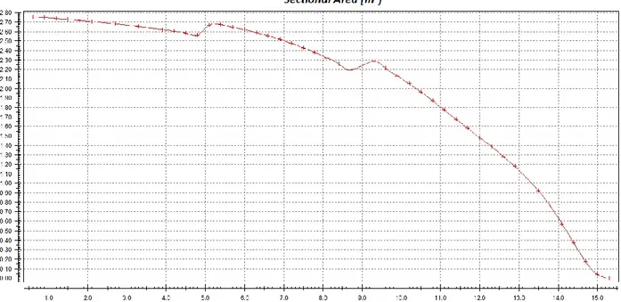
The sectional are to the project draught is shown in Figure 3 for the mother hull. There is not discontinuity along the longitudinal position of the sectional area.
Figure 3 - Sectional Area along the longitudinal position to the Displacement of Project - Model A at full scale
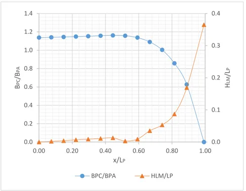
In order to describe appropriately the geometry of the hull, besides the traditional characteristics, other geometric dimensions are also described, according to Larsson and Eliasson (Larsson and Eliasson, 2000). Three principal curves and several parameters based on the projected area AP are reported for every model. AP is the projection of the bottom part of the hull (part between the keel and the chine) on a horizontal plane (OXY in this case). Respect this area four dimensions could be defined: BPT (transom projected Beam), BPX (maximum projected beam), BPC (beam at a generic X position in longitudinal direction) and the Projected Length LP (Figure 4). In the Figure 5 is reported the definition of the deadrise angle β. The last parameter is the Height of the buttock line (HLM) at 0.25 BPA from the symmetry plane (Figure 6). This height is measured respect to a line tangent to the bottom of the hull at stern.
________________________________________________________________________________
Felice Sfravara 17
Figure 5 - Deadrise Angle
Figure 6 - Buttock at 0,25 BPA from the symmetry plane and definition of the HLM
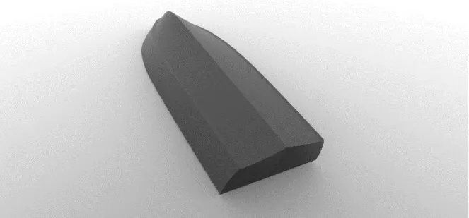
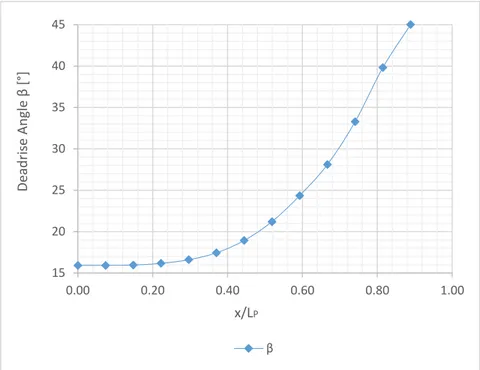
The Figure 7 shows a CAD representation of the original hull form and in Figure 8 is reported the deadrise angle in function of the longitudinal position. The first part of the hull has a constant deadrise angle, it starts to increase to a 30% of the Lp. As shown in Figure 9, the beam along the longitudinal position is constant for the most part of Lp. In the same Figure, the height of longitudinal profile is zero for the first 40% of Lp.
________________________________________________________________________________
Felice Sfravara 18
Figure 8 - The deadrise along x/LP - Model A
Figure 9 - The distribution of the projected beam and the distribution of HLM along x/LP - Model A
The design philosophy, for this kind of ACS, was to imagine a cavity that could take advantage to the bottom low pressure, typical of planing hulls. This low pressure develops naturally aft the pressure peak in correspondence of the stagnation line (Morabito, 2014). In this region, the total pressure can be near to the local hydrostatic pressure, and, in presence of steps, can reach negative values (in relative terms).
15 20 25 30 35 40 45 0.00 0.20 0.40 0.60 0.80 1.00 De ad ris e An gle β [ °] x/LP β 0.0 0.1 0.2 0.3 0.4 0.0 0.2 0.4 0.6 0.8 1.0 1.2 1.4 0.00 0.20 0.40 0.60 0.80 1.00 H LM /L P B PC /B PA x/LP BPC/BPA HLM/LP
________________________________________________________________________________
Felice Sfravara 19
Unlike the traditional displacement ACS, in order to take advantage of this phenomenon, the cavity proposed by the author, is much less deep and the ventilation plant is very small with a great advantage in terms of power saving. In this way, rather than an air-cushion, the idea was to create an air-layer. This approach allows obtaining a bottom cavity that does not alter very much the original hull geometries and that is less invasive, in particular for the seakeeping and the increment of the wetted surface.
The first design of the bottom cavity has been a single large hollow, called “stepped hull” (Model B). The body plan of the hull is reported in Figure 10 and the hydrostatic characteristics are reported in Figure 12. The chine of the hull is the same of the original one and, as shown in the body plan the step has been added to 8 m (model scale) away from the stern.
________________________________________________________________________________
Felice Sfravara 20
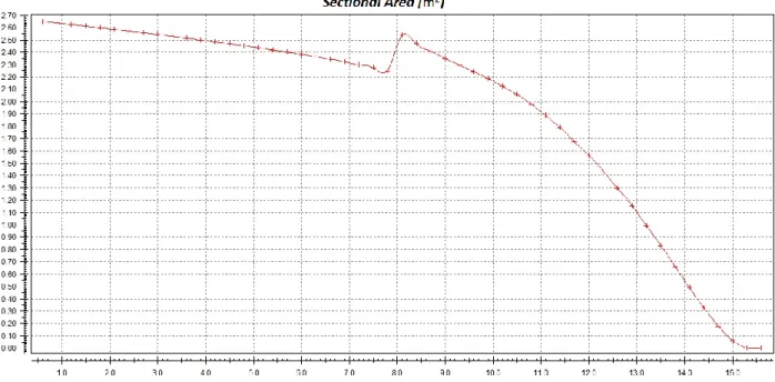
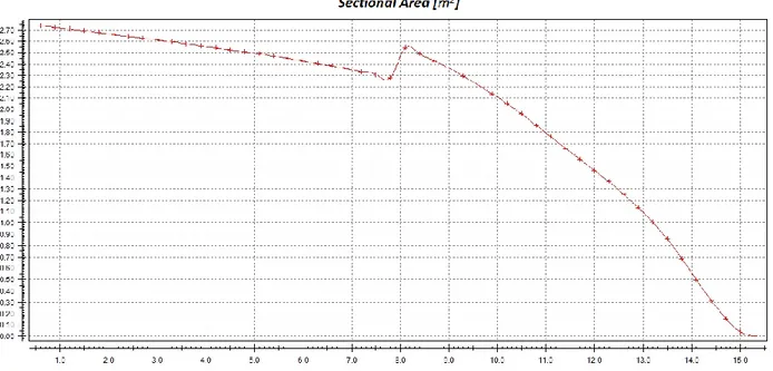
In Figure 11 is shown the sectional area at full scale with the presence of the discontinuity in the position of the step to a position reported in LST Table 2.
Figure 11 - Sectional Area along the longitudinal position to the Displacement of Project - Model B at full scale
Figure 12 - Hydrostatic quantities of Model B at full scale
0 1 2 3 4 5 6 7 8 9 10 11 12 13 14 15 16 17 0.1 0.3 0.5 0.7 0.9 1.1 1.3 1.5 0.1 0.2 0.3 0.4 0.5 0.6 0.7 0.8 0.9 1 1.1 1.2 1.3 1.4 1.5 0 5 10 15 20 25 30 35 40 45 50 55 60 65 70 75 80 85 90 Δ [t] Volume [m^3] AWL [m^2] S [m^2] KMl [m] LWL [m] BWL [m] LCB [m] VCB [m] LCF [m] KMt [m] Mu [t*m/cm] Δu [t/cm]
________________________________________________________________________________
Felice Sfravara 21
In Matveev (Matveev, 2015) a study that concerns the influence of the height of the step and the position in the bottom has been investigated, in the conclusions of this paper it highlights the lack of experimental data in cavity ship with stepped solution. The principal idea of this solution is related to ventilation behind a wedge attached to a horizontal wall. Figure 13 shows hull form of the stepped hull with a focus on the surface zone interested by air cavity. The Table 2 shows the main dimensions of this model, with position of the step, surface of the step and surface of the nozzles. In this case the percentage between the surface of the step and surface of the nozzles (fill rate) is 92.5%. The number of nozzles is 40.
Figure 13 - Monostep solution (Model B)
Dimensions Ship Model Unit
LWL 14.96 2.49 m LP 16.2 2.7 m BWL 4.32 0.72 m BPX 3.72 0.62 m BPA 3.2 0.53 m BPT 3.66 0.61 m T 1.00 0.17 m Δ 34 0.15 t S 70.9 1.97 m2 xG (% of LOA) 36.49 % 36.49 % - AP 51.84 1.44 m2 NST 1 1 - LST 8.00 1.33 m
________________________________________________________________________________ Felice Sfravara 22 SST 0.332 0.009 m2 NIN 40 40 - BIN x HIN 0.085 x 0.09 0.0142 x 0.015 m x m SIN 0.307 0.0085 m2
Table 2 - Main dimensions Model B
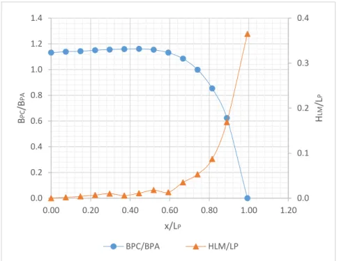
In Figure 14 are reported the graphs with the geometric parameters. The trend of the deadrise angle is the same of the original hull. There is a discontinuity of the parameter HLM for the presence of the step (Figure 15). The idea for this model was to keep the same principal parameters of the original hull.
Figure 14 - The deadrise and on right along x/LP - Model B
15 20 25 30 35 40 45 0.00 0.20 0.40 0.60 0.80 1.00 De ad ris e An gle β [ °] x/LP β
________________________________________________________________________________
Felice Sfravara 23
Figure 15 - the distribution of the projected beam and the distribution of HLM along x/LP - Model B
A second configuration (Model C) is a multi-steps solution. The body plan of the model is showed in Figure 16 and the hydrostatic quantities in Figure 17. The position of the steps is 5 m and 9 m away from the stern.
Figure 16 - Lines plan reported in real scale of Model C
0.0 0.1 0.2 0.3 0.4 0.0 0.2 0.4 0.6 0.8 1.0 1.2 1.4 0.00 0.20 0.40 0.60 0.80 1.00 H LM /L P B PC /B PA x/LP BPC/BPA HLM/LP
________________________________________________________________________________
Felice Sfravara 24
Figure 17 - Hydrostatic quantities of model C in real scale
In the case of Model C the sectional area curve is different respect to each other. In this case there are two discontinuities, in the position of the first step and in the position of the second step as shown in Figure 18.
Figure 18 - Sectional Area along the longitudinal position to the Displacement of Project - Model C at full scale
0 1 2 3 4 5 6 7 8 9 10 11 12 13 14 15 16 17 0.1 0.3 0.5 0.7 0.9 1.1 1.3 1.5 0.1 0.2 0.3 0.4 0.5 0.6 0.7 0.8 0.9 1 1.1 1.2 1.3 1.4 1.5 0 5 10 15 20 25 30 35 40 45 50 55 60 65 70 75 80 85 90 Δ [t] Volume [m^3] AWL [m^2] S [m^2] KMl [m] LWL [m] BWL [m] LCB [m] VCB [m] LCF [m] KMt [m] Mu [t*m/cm] Δu [t/cm]
________________________________________________________________________________
Felice Sfravara 25
This kind of solution is suggested if the air-cavity length could not be extended to the whole hull length, principally to low speed conditions. A series of steps are used in the bottom of the hull (Figure 19), with different injections of air along the vessel length. The multi-step solution requires more modifications in the bottom of the original hull, respect to mono-step solution but the air cavity should be more stable. The Table 3 shows the main dimensions of this model, with position of the two steps, relative area of the steps and total area of the nozzles. The number of the nozzles is 8 for the first step and 8 for the second step, in the first case the fill rate is 93 % and in the second step is 92 %. In Figure 20, the three parameters above described are represented respect to x/LP. A parametric CAD has been developed for a faster reconstruction of the geometry model and for eventual changes in the future (Figure 19).
Figure 19 - Multi-steps hull (Model C)
Dimensions Ship Model Unit
LWL 14.908 2.485 m LP 16.2 2.7 m BWL 4.314 0.719 m BPX 3.72 0.62 m BPA 3.2 0.54 m BPT 3.66 0.61 m T 1.000 0.167 m Δ 34 0.153 t S 70.7 1.963 m2 xG (% of LOA) 35.88 % 35.88 % - AP 52.2 1.45 m2 NST 2 2 -
________________________________________________________________________________
Felice Sfravara 26
Main Dimensions STEP 1
LST1 5.00 0.833 m
SST1 0.150 0.004 m2
NIN1 8 8 -
BIN x HIN 0.38 x 0.046 0.063 x 0.0076 m x m
SIN1 0.14 0.0038 m2
Main Dimensions STEP 2
LST2 9.00 1.5 m
SST2 0.234 0.0065 m2
NIN2 8 8 -
BIN x HIN 0.3 x 0.09 0.05 x 0.015 m x m
SIN2 0.216 0.006 m2
Total Contribution of Steps
SIN 0.356 0.0098 m2
Table 3 - Main Dimensions of Model C
In the case of Model C, the deadrise is slightly different with respect to the original hull because of the presence of two steps (Figure 20). The beam of the chine have been maintained constant with respect to the original hull. The value of HLM is different respect to the original hull. There are two discontinuities and the longitudinal profile is modified in order to accommodate these two steps (Figure 21).
Figure 20 - The deadrise along x/LP - Model C
15 20 25 30 35 40 45 0.00 0.20 0.40 0.60 0.80 1.00 De ad ris e An gle β [ °] x/LP β
________________________________________________________________________________
Felice Sfravara 27
Figure 21 - The distribution of the projected beam and the distribution of HLM along x/LP - Modelc C
The last configuration (Model D) is obtained with a cavity identical to that of Model B, but with the insertion of longitudinal rails (Figure 25). The body plan is reported in Figure 22 and the hydrostatic quantities are reported in Figure 23.
Figure 22 - Lines plan in real scale of Model D
0.0 0.1 0.2 0.3 0.4 0.0 0.2 0.4 0.6 0.8 1.0 1.2 1.4 0.00 0.20 0.40 0.60 0.80 1.00 1.20 H LM /L P B PC /B PA x/LP BPC/BPA HLM/LP
________________________________________________________________________________
Felice Sfravara 28
Figure 23 - Hydrostatic quantities of Model D in real scale
The sectional area to the displacement of project is reported in Figure 24. The position of the step is shown in this graph with the discontinuity to the correspondent position.
Figure 24 - Sectional Area along the longitudinal position to the Displacement of Project – Model D
0 1 2 3 4 5 6 7 8 9 10 11 12 13 14 15 16 17 0.1 0.3 0.5 0.7 0.9 1.1 1.3 1.5 0.1 0.2 0.3 0.4 0.5 0.6 0.7 0.8 0.9 1 1.1 1.2 1.3 1.4 1.5 0 5 10 15 20 25 30 35 40 45 50 55 60 65 70 75 80 85 90 Δ [t] Volume [m^3] AWL [m^2] SW [m^2] KMl [m] LWL [m] BWL [m] LCB [m] VCB [m] LCF [m] KMt [m] Mu [t*m/cm] Δu [t/cm]
________________________________________________________________________________
Felice Sfravara 29
A great problem for the stability of the air-cavity is the escape of the air in transversal direction, due to the V-shape of the hull. The presence of longitudinal rails allows channeling the flow reducing the possibility to escape from transversal direction. The numbers and dimensions of these channels depend to the dimension of longitudinal rails. The Table 4 shows the main dimensions of this model. In this case the area of the step where is possible to obtain air injection is reduced by the section area of the longitudinal rails, so the area is 0.304 m2. The fill rate respect to this area is 92 %. In the table are reported the dimensions of rectangular section of the rail and the distance between each other and in Figure 26 the three parameters above described are represented respect to x/LP.
Figure 25 - Longitudinal rails hull (Model D)
Dimensions Ship Model Unit
LWL 14.884 2.481 m LP 16.2 2.7 m BWL 4.314 0.719 m BPX 3.72 0.62 m BPA 3.2 0.54 m BPT 3.66 0.61 m T 1.000 0.167 m Δ 34 0.153 t S 78.6 2.182 m2 xG (% of LOA) 35.92 % 35.92 % - AP 52.2 1.45 m2 NST 1 1 - LST 8.00 1.333 m
________________________________________________________________________________ Felice Sfravara 30 SST 0.304 0.0084 m2 NIN 10 10 - B x H 0.31 x 0.09 0.051 x 0.015 m x m SIN 0.279 0.0077 m2
Longitudinal Rails Dimensions
N 8 8 -
BR x HR 0.041 x 0.059 0.007 x 0.01 m x m
TDR 0.340 0.056 m
Table 4- Main Dimensions of Model D
The deadrise trend shown in Figure 26 is the one without considering the deadrise of the rails.The rails have a bottom surface parallel to the one of the hull. They have not been designed for to decrease the average value of the deadrise. This choice has been done in order to keep the average deadrise equal to original one. These rails have been designed only for better directing the air flow during the injection.
Figure 26 - The deadrise and along x/LP - Model D
Figure 26 shows the trend for the beam of the chine and the HLM and these two parameters are the same of the original hull.
15 20 25 30 35 40 45 0.00 0.20 0.40 0.60 0.80 1.00 Dead ris e An gle β [ °] x/LP β
________________________________________________________________________________
Felice Sfravara 31
Figure 27 - The distribution of the projected beam and the distribution of HLM along x/LP - Model D
In all the proposed solutions, the percentage of area for air flow injection is between 90 % and 93 % of the total area of the correspondent step. In general, the addition of element as steps or rails increases the wetted surface (Figure 28), this at expense of friction drag, because this resistance is heavily dependent by that area. The major increase of the wetted surface is in Model D, due to the presence of the longitudinal rails. The other dimensions are the same for every model.
Figure 28- Wetted Surface Area
The general idea during the phase of design was to keep all the principal dimensions of modified hulls (angle of deadrise, BPC and HLM) equal to the original one in order to evaluate the difference of the performances caused by only the different of the bottom shapes. It clears that this condition was difficult for the hull with two steps where the geometry is slightly different with respect to the other three. 0.0 0.1 0.2 0.3 0.4 0.0 0.2 0.4 0.6 0.8 1.0 1.2 1.4 0.00 0.20 0.40 0.60 0.80 1.00 H LM /L P B PC /B PA x/LP BPC/BPA HLM/LP 62 64 66 68 70 72 74 76 78 80 Model A-B We tte d S u rf ac e m 2
________________________________________________________________________________
Felice Sfravara 32
5.3 Model manufacturing
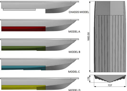
The number of models for the towing tank test is four, but in order to reduce the costs, a single chassis model has been defined, and the four different bottom hulls have been fixed to the chassis with fasteners (Figure 29). The design of the different bottoms has been normalized to an only length in order to simplify the setup of the chassis. The principal dimensions are shown in Figure 29 while picture of the chassis model is shown in Figure 30.
Figure 29 - Chassis model and different bottom on left - Dimensions in mm of unified bottom on right
________________________________________________________________________________
Felice Sfravara 33
The four bottom models are shown in Figure 31. Respectively from left to right there are: the original hull, the Model B with a single step, the model C with two steps and the last model (Model D) with the presence of rails.
Figure 31 – Bottom models
The material of the model is Glass Reinforced Plastic and wood. The chassis and the different bottom hull are sandwich structures, with core in polystyrene and skins with different layer of fiberglass. Two parts have been obtained inside the chassis model for the connection with the dynamometric carriage, the central one for the entrainment of the model by the carriage and the anterior one for keeping aligned the model during the tests. According to the requirements of these tests, a constant and regulated air supply has been delivered to the model (Figure 32). The air was to be delivered by a centrifugal system with a maximum flow rate of 11 m3/min. The flow of the air and the angular velocity of the rotor are controlled, with a closed loop the necessary flow is delivered to the system.
________________________________________________________________________________
Felice Sfravara 34
The model has been designed in order to accommodate all necessary auxiliaries for making sea trials. In order to do this kind of trials the model can be equipped with steering and propulsion system. The steering system is defined by two rudders steered by one electrical motor with possibility to rotate between +/- 45 degrees. The propulsion system is defined by two contra-rotating propellers with five blades and 190 mm of diameter, the rotation of propellers is covered by two electrical motors with a total power of 3kW. The propulsion and steering system are shown in Figure 33.
Figure 33 – Rudders and Propellers
The power for the all elements on board is supplied by a system of 20 lithium batteries (two packs are shown in Figure 34) with a total power of 10.24 kWh in three different tension (12/24/48 V). The entire system is governed by an in-house software developed by ATEC robotics thanks to a Wireless system.
________________________________________________________________________________
Felice Sfravara 35
Figure 34 - Lythium Batteries
In order to keep safe the equipment inside the hull during the sea trials, a cover has been designed for the hull and for the steering system. The general dimensions are shown in Figure 35.
Figure 35 - General dimensions of the model
The Figure 36 (on left) shows a 3D representation of the model with all components (propellers, rudders, cover) and in the same picture, on right, is shown a picture with the real model. The porthole in the center of the ship has been designed in order to position the system for the wireless signal.
________________________________________________________________________________
Felice Sfravara 36
Figure 36 – Complete arrangements of the model
During the tests of this research, the model has been equipped only with the air injection system and the hull has been tested without appendages as shown in Figure 37. The total amount of weight of the model has to be equal to 0.155 t, in order to respect the proper immersion in geometric similarity with the real boat. The air is supplied via a piping system to the nozzles; the more difficult accommodation of air supplier has been for the Model C, for the presence of two steps with two different piping systems.
Figure 37 - The hull model in the towing tank
The principal aim of the tests is to obtain a better knowledge of the air ventilation phenomena, respect to different bottom hull shape. The tests focus on extrapolation of the resistance curves, varying the velocities and the air flow rate. The maximum velocity of the model depend, by means
________________________________________________________________________________
Felice Sfravara 37
the similitude of the Froude number (Eq.5.11), to the maximum velocity of the yacht, taking into account the maximum velocity possible for the carriage system.
𝐹𝑛 = 𝑉𝑆 √𝑔𝐿𝑆 = 𝑉𝑀 √𝑔𝐿𝑀 (𝐸𝑞. 5.11) 𝑉𝑀 = 𝑉𝑆 √𝜆 (𝐸𝑞. 5.12)
The maximum velocity of the yacht is 32 knots (16.49 m/s) so, for the (Eq.5.12), the maximum velocity of the model is 6.72 m/s. This velocity is inside the work range of the towing tank. The complete series of velocities for every single trial is reported in Table 5. For each trial, the model hull and flow rate are fixed.
VM (m/s) VS (m/s) VS (knots) Fn 2.520 6.17 12.0 0.510 3.150 7.71 15.0 0.638 3.780 9.26 18.0 0.765 4.410 10.80 21.0 0.893 5.040 12.34 24.0 1.020 5.670 13.89 27.0 1.148 6.300 15.43 30.0 1.275 6.720 16.46 32.0 1.360
Table 5 - Series of velocities for single trial
The reference model was the Model A (original hull) and for this model only three trials for resistance curves have been conducted to three different displacements (Figure 38). For each model with air-cavity, were carried out one trial without air flow and six trials with different air flow rate. A total of 24 trials were carried out for a total amount of 192 tests conducted. In the Table 6 are reported the flow rate and displacement for every trial. The flow rate is in the range between 5500 l/min and 10500 l/min. The displacement is correspondent to 34 t of the yacht.
Number of Trial Model Flow rate [l/min] ∆M [t] ∆S [t]
Trial 1 Model A No air 0.139 30.9
Trial 2 Model A No air 0.153 34
Trial 3 Model A No air 0.167 37
Trial 4 Model B No air 0.153 34
Trial 5 Model B 5500 0.153 34 Trial 6 Model B 6500 0.153 34 Trial 7 Model B 7500 0.153 34 Trial 8 Model B 8500 0.153 34 Trial 9 Model B 9500 0.153 34 Trial 10 Model B 10500 0.153 34
Trial 11 Model C No air 0.153 34
Trial 12 Model C 5500 0.153 34
Trial 13 Model C 6500 0.153 34
________________________________________________________________________________
Felice Sfravara 38
Trial 15 Model C 8500 0.153 34
Trial 16 Model C 9500 0.153 34
Trial 17 Model C 10500 0.153 34
Trial 18 Model D No air 0.153 34
Trial 19 Model D 5500 0.153 34 Trial 20 Model D 6500 0.153 34 Trial 21 Model D 7500 0.153 34 Trial 22 Model D 8500 0.153 34 Trial 23 Model D 9500 0.153 34 Trial 24 Model D 10500 0.153 34
Table 6 - Trials conducted. For each trial eight different velocities have been carried out
Figure 38 – A towing tank test on model A
5.4 Results and Discussion of experimental Tests
The trials produced series of resistance curves that are an important starting point for a better understanding of the behavior of the model with and without air. The first group of trials concerns the Model A i.e. the original mother-hull. These tests have been conducted with three different displacement. The values of displacement of the full-scale boat were 30.9 t, 34.0 t and 37.0 t. The curves are similar but there is a natural increase of resistance with the increase of the displacement. All the curves are reported in model scale quantities.
________________________________________________________________________________
Felice Sfravara 39
Figure 39 - Drag curves for Model A
An estimation of the Drag components has been conducted for the mother-hull (Model A), in the 34 t configuration (Figure 40). Since the model is not ventilated, the theory for the Drag components evaluation is well consolidated. This helps to understand the importance of the air injection, especially at high Froude Numbers, for which Frictional Drag can reach almost the 50 %.
120 140 160 180 200 220 240 260 280 300 320 2.50 3.00 3.50 4.00 4.50 5.00 5.50 6.00 6.50 7.00 Drag re sis ta n ce [ N ] Velocity [m/s]
________________________________________________________________________________
Felice Sfravara 40
Figure 40 – Drag components for Model A (34 t)
The Model B has been tested to 34 t conditions (0.153 t in scale model) and the trend of the curves without air injection is very similar to the one of the mother hull. Figure 41 shows the general trend of all curves tested to different flow rate. There is an important drop of the curves between the no-air test and all others tests with no-air. The drop of the curves is little and almost constant respect to the flow rate for an interval of velocities between the first tested velocity and about 5.04 m/s, after this velocity the decrease of power requested is evident. This trend is shown for both of models in Figure 41. 0 0.1 0.2 0.3 0.4 0.5 0.6 0.7 0.8 0.9 1 1.1 2.00 2.50 3.00 3.50 4.00 4.50 5.00 5.50 6.00 6.50 7.00 Drag comp o n en ts [ % ] Velocity [m/s]
________________________________________________________________________________
Felice Sfravara 41
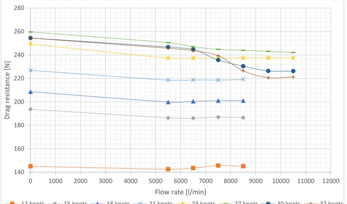
Figure 41 - Drag curves to vary flow rate- Model B
A better understanding of the influence of the flow rate on the resistance is shown in Figure 42. In this graph the curves have the same trend until to the velocity of 24 knots. The curves to a low velocity are not influenced by the flow rate, the decrease of resistance is the same. Over the 24 knots, the influence of flow rate is important and the decrease is highly influenced by the air flow rate. 140 160 180 200 220 240 260 2.50 3.00 3.50 4.00 4.50 5.00 5.50 6.00 6.50 7.00 Drag re sis ta n ce [ N ] Velocity [m/s]