Calibration and performances of in-situ gamma ray spectrometer

(1)

Calibration and performances of in-situ gamma ray spectrometer

by

Manjola Shyti

Submitted to

The University of Ferrara

(Faculty of Mathematics, Physics and Natural Sciences)

for the degree of

PhD in Physics

March 2013

(2)

List of figures and tables

Chapter 1

Figure 1.1: exponential decay of activity.

Figure 1.2: temporal trend of the number of parent atoms and daughter atoms in a radioactive sample.

Figure 1.3: qualitative representation of the secular equilibrium concept. The atoms of 238_{U subject to decay are} represented as a fluid which is poured into the container of 234_{Th. In secular equilibrium conditions the outgoing flow} from the container of 234_{Th, corresponding to the number of atoms of}234_{Th subject to decay, will be equal to the} incoming flow, corresponding to the number of atoms of 234_{Th produced by the decay of}238_{U. If the decay chain of}238_U is in secular equilibrium in its entirety, equality between the incoming and the out coming flow is valid for every element in the chain.

Figure 1.4: example of three Poisson distributions with mean value equal to 1, 5 and 10. It is observed that as average value increase, the Poisson distribution is close to Gauss ones.

Figure 1.5: binding energy per nucleon of common isotopes.

Figure 1.6: representation of the stable nuclei, marked with green squares, as a function of the atomic number Z. The stable nuclei are arranged on the straight line Z = N for values of Z less than 20; for Z > 20, the stability curve towards the axis N, highlighting the greater stability of the nuclei with a number of neutrons greater than the number of protons. Figure 1.7: three dimensional representation of valley of stability.

Figure 1.8: schematic representation of decay and - decay of 227_Th. Figure 1.9: alpha spectrum associated with the decay of 227_Th.

Figure 1.10: schematic representation of β-_{decay; β}−_{(on the left) and β}+ _{(on the right).} Figure 1.11: schematic representation decay for 137_Cs.

Figure 1.12: schematic representation of electron capture process.

Figure 1.13: representation of the reactions involved in the interaction of particles of primary cosmic rays with the atmosphere, giving rise to secondary cosmic rays.

Figure 1.14: potassium decay modes. Figure 1.15: uranium decay chain. Figure 1.16: thorium decay chain.

Figure 1.17: decay chain of 238_{U where are highlighted the possible points in which the condition of secular equilibrium} is broken.

Figure 1.18: decay chain of 232_{Th where are highlighted the possible points in which the condition of personal} equilibrium is broken.

(5)

Chapter 2

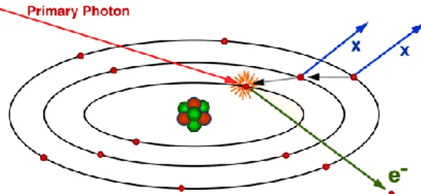
Figure 2.1: schematic representation of the photoelectric effect and the subsequent emission of X-ray characteristic. Figure 2.2: schematic representation of the scattering between a photon and a free electron.

Figure 2.3: schematic of the Compton scattering process.

Figure 2.4: cross section for the photoelectric effect, Compton scattering and pair production and the total cross section for an atom of Lead as a function of the photon energy.

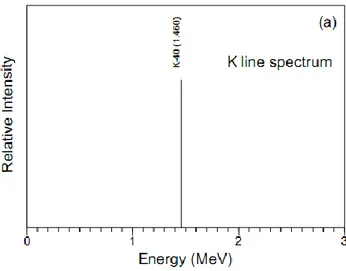
Figure 2.5: gamma ray emission line spectra of potassium (IAEA-TECDOC-1363, 2003). Figure 2.6: gamma ray emission line spectra of uranium (IAEA-TECDOC-1363, 2003). Figure 2.7: gamma ray emission line spectra of thorium (IAEA-TECDOC-1363, 2003).

Figure 2.8: simulated potassium fluence rates at 300 meter height (IAEA-TECDOC-1363, 2003). Figure 2.9: simulated uranium fluence rates at 300 meter height (IAEA-TECDOC-1363, 2003). Figure 2.10: simulated thorium fluence rates at 300 meter height (IAEA-TECDOC-1363, 2003). Figure 2.11: example of energy resolution for a gamma rays spectrometer (IAEA-TECDOC-1363, 2003). Figure 2.12: schematic representation of a scintillation detector.

Figure 2.13: schematic representation of the energy levels of singlet and triplet in organic scintillators.

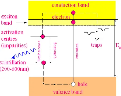
Figure 2.14: schematic representation of the band structure of an inorganic scintillator. The centers activators introduce energy levels within the energy gap between the valence band and the conduction band.

Figure 2.15: dependence of the light emission of scintillating crystals by temperature. Figure 2.16: scheme of a photomultiplier coupled to a scintillator.

Figure 2.17: schematic representation of a p-n junction.

Chapter 3

Figure 3.1: framework of the basin of Ombrone in respect to Tuscany region.

Figure 3.2: geological map of the Basin of Ombrone River 1:500000 highlighted with the points in which were carried out the measurements of natural radioactivity.

Figure 3.3: geological map of the commune of Schio.

Figure 3.4: coordinate system used in the theoretical calculations for the variation of detector count rate with its height respect to the ground.

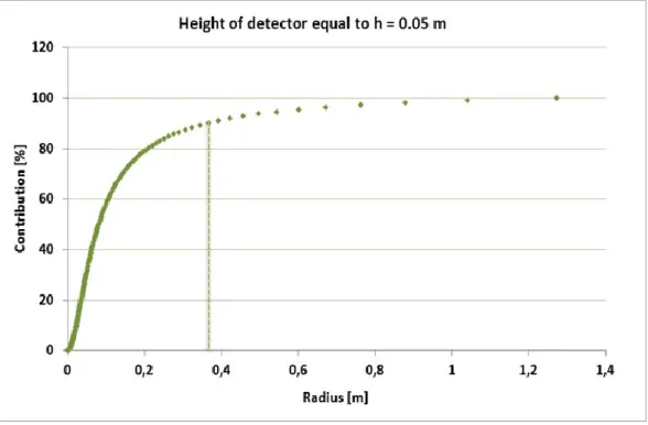
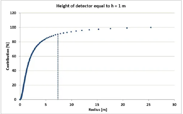
Figure 3.5: percentage contribution of the signal received by the detector placed at a height of 0.05 m. Figure 3.6: percentage contribution of the signal received by the detector placed at a height of 0.5 m. Figure 3.7: percentage contribution of the signal received by the detector placed at a height of 1 m.

(6)

Figure 3.8: the ZaNaI_1.0Lsystem configuration set-up in a backpack. Figure 3.9: energy windows for the WAM analysis of a gamma spectrum. Figure 3.10: the sensitive spectra obtained through the FSA with NNLS constraint. Figure 3.11: example of acquisition of the spectrum with backpack placed on the ground.

Figure 3.12: example of acquisition of the spectrum with backpack placed on the tripod at 1 m height above the ground. Figure 3.13: example of acquisition of the spectrum with backpack placed on the shoulders.

Figure 3.14: example of the soil samples arrangement with respect to the central point in which is realized the measurement of gamma-ray spectroscopy in situ.

Table 3.1: typical concentrations of constructed pads used to calibrate in-situ gamma-ray spectrometers (IAEA 1990). Table 3.2: standard gamma ray energy windows recommended for natural radioelement mapping.

Table 3.3: the average of the distribution of natural radioisotopes concentration. The errors correspond to one standard deviation. The conversion factors from Bq/kg are obtained by (IAEA-TECDOC-1363, 2003): 1%=313 Bq/kg for potassium, 1 ppm=13.25 Bq/kg for uranium and 1 ppm=4.06 Bq/kg for thorium.

Table 3.4: standard pedological parameters to define in the campaign.

Table 3.5: environmental parameters monitored during the in situ measurement.

Chapter 4

Figure 4.1: ventilated oven used to dry the soil samples.

Figure 4.2: soil samples ready to be analyzed with MCA_Rad system. Figure 4.3: MCA_Rad system composed by two coupled HPGe detectors.

Figure 4.4: MCA_Rad system shielding of HPGe detectors composed by copper and lead.

Figure 4.5: MCA_Rad system background spectra (live time 100 h) without (red) and with (green) shielding showing a reduction of two order of magnitudes.

Figure 4.6: absolute efficiency curve for the MCA_Rad system obtained by fitting the corrected values for coincidence summing with equation 2.16. Apparent efficiencies of 152_{Eu (blue triangles) and}56_{Co (green squares) are also presented.} Figure 4.7: loader of samples and instrumentation for reading the bar code of MCA_Rad system.

Table 4.1: the features of two detectors used for design of MCA_Rad system (these values are measured by the manufacturer).

Chapter 5

Figure 5.1: representation of the total measured spectrum obtained by the superposition of the fundamental spectra of cesium, potassium, uranium and thorium, and the background spectrum.

(7)

Figure 5.2: frequency histogram of the abundances of 40_{K obtained for the 400 soil sampling fitted with a log-normal} function.

Figure 5.3: the correlation between the abundance of K measured on sample using HPGe detectors and the abundance of K measured in-situ using ZaNaI_1.0L placed on the ground is described by the relationship KZaNaI = (1.16 ± 0.05) KHPGe with r2_{= 0.90.}

Figure 5.4: the correlation between the abundance of eU measured on sample using HPGe detectors and the abundance of eU measured in-situ using ZaNaI_1.0L placed on the ground is described by the relationship eUZaNaI = (0.85 ± 0.11) eUHPGe with r2 = 0.64.

Figure 5.5: the correlation between the abundance of eTh measured on sample using HPGe detectors and the abundance of eTh measured in-situ using ZaNaI_1.0L placed on the ground is described by the relationship eThZaNaI = (0.97 ± 0.12) eThHPGe with r2 = 0.80.

Figure 5.6: the correlation between the abundance of K measured on sample using HPGe detectors and the abundance of K measured in-situ using ZaNaI_1.0L placed on the tripod is described by the relationship KZaNaI = (1.11 ± 0.05) KHPGe with r2_{= 0.88.}

Figure 5.7: the correlation between the abundance of eU measured on sample using HPGe detectors and the abundance of eU measured in-situ using ZaNaI_1.0L placed on the tripod is described by the relationship eUZaNaI = (0.75 ± 0.10) eUHPGe with r2_{= 0.66.}

Figure 5.8: the correlation between the abundance of eTh measured on sample using HPGe detectors and the abundance of eTh measured in-situ using ZaNaI_1.0L placed on the tripod is described by the relationship eThZaNaI = (0.92 ± 0.11) eThHPGe with r2_{= 0.79.}

Figure 5.9: the correlation between the abundance of K measured by placing the ZaNaI_1.0L on ground and on tripod is described by the relationship Kground= (0.93 ± 0.03) Ktripod with r2 = 0.98.

Figure 5.10: the correlation between the abundance of eU measured by placing the ZaNaI_1.0L on ground and on tripod is described by the relationship eUground= (0.87 ± 0.03) eUtripod + (0.31 ± 0.14) with r2_{= 0.73.}

Figure 5.11: the correlation between the abundance of eTh measured by placing the ZaNaI_1.0L on ground and on tripod is described by the relationship eThground= (0.94 ± 0.06) eThtripod with r2_{= 0.96.}

Figure 5.12: the correlation between the abundance of 137_{Cs measured by placing the ZaNaI_1.0L on ground and on} tripod is described by the relationship 137_Cs

ground= (0.81 ± 0.02) 137Cstripod with r2 = 0.95.

Figure 5.13: the correlation between the abundance of K measured by placing the ZaNaI_1.0L on ground and on shoulder is described by the relationship Kground= (0.82 ± 0.01) Kshoulder + (0.08 ± 0.01) with r2_{= 0.97.}

Figure 5.14: the correlation between the abundance of eU measured by placing the ZaNaI_1.0L on ground and on shoulder is described by the relationship eUground= (0.84 ± 0.01) eUshoulder + (0.13 ± 0.03) with r2 = 0.98.

Figure 5.15: the correlation between the abundance of eTh measured by placing the ZaNaI_1.0L on ground and on shoulder is described by the relationship eThground= (0.83 ± 0.02) eThshoulder with r2_{= 0.97.}

Figure 5.16: the correlation between the abundance of 137_{Cs measured by placing the ZaNaI_1.0L on ground and on} shoulder is described by the relationship 137_Cs

(8)

Figure 5.17: for 0-50% vegetative cover case: the correlation between the abundance of Th measured by placing the ZaNaI_1.0L on ground and on shoulder is described by the relationship Thground= (0.83 ± 0.02) Thshoulder with r2_{= 0.99.} Figure 5.18: for 50-100% vegetative cover case: the correlation between the abundance of Th measured by placing the ZaNaI_1.0L on ground and on shoulder is described by the relationship Thground= (0.85 ± 0.02) Thshoulder with r2 = 0.97. Figure 5.19: for 0-50% vegetative cover case: the correlation between the abundance of 137Cs measured by placing the ZaNaI_1.0L on ground and on shoulder is described by the relationship 137_{Csground= (0.72 ± 0.02)}137_{Csshoulder with r}2₌ 0.97.

Figure 5.20: for 50-100% vegetative cover case: the correlation between the abundance of 137Cs measured by placing the ZaNaI_1.0L on ground and on shoulder is described by the relationship 137_{Csground= (0.77 ± 0.01)}137_{Csshoulder with r}2₌ 0.96.

Table 5.1: conversion factors between specific activity and concentrations of K, eU and eTh.

Table 5.2: relationships between the parameters of the distribution in the original scale and in that logarithmic one. Table 5.3: the correlation parameters obtained for in-situ measurements on ground and laboratory measurements. Table 5.4: correlation between measurements in-situ acquisition on tripod and in the laboratory.

Table 5.5: correlation parameters between in-situ measurements on ground and on tripod. Table 5.6: correlation parameters between in-situ measurements on ground and on shoulder.

Table 5.7: correlation parameters between in-situ measurements on ground and on shoulder for two classes of vegetative coverage.

Chapter 6

Table 6.1: correlation between ZaNaI_1.0L measurements obtained by placing the detector on ground and on tripod respect to laboratory measurements.

Table 6.2: attenuation correction due to air for in-situ measurements at tripod (1m height).

(9)

Abstract

Since 1896, when Henri Becquerel discovered that penetrating radiation was given off in the radioactive decay of uranium, the studies on radioactivity have been an interest of scientific world. With the spread of nuclear technologies applied to energy, health and industrial production, the theme of environmental radioactivity monitoring increasingly is becoming important to the policies of the health public protection both national and European level. Italy is required to comply with the recommendation of the European Commission of 8 June 2000 on the application of Article 36 of the Euratom Treaty concerning the monitoring of levels of radioactivity in the environment for the purpose of assessing the exposure of the population as a whole. In addition, the World Health Organization has identified the first group of carcinogens gas 222Rn, which is considered the second leading cause, after smoking, of lung tumors. In our environment there are various sources of radioactivity that can be natural or artificial origin. Gamma-ray spectrometry is a widely used and powerful method that can be employed both to identify and quantify radionuclides. The purpose of this work is calibration and performances of in situ a portable gamma ray spectrometer.

In the first chapter I have given the necessary concepts for understanding the phenomenon of radioactivity. Qualitatively has been described the process of radioactive decay and its three types which can occur in nature. Three categories of environmental radionuclides, cosmogenic, primordial and man-made are discussed. We are exposed to environmental radiation from different sources. The origin of radioactivity in the environment can be divided into two main sources: (a) natural and (b) man-made sources. Mostly the naturally occurring radiation arises from terrestrial radioactive nuclides that are widely distributed in the earth’s crust and extra-terrestrial sources arising from cosmic ray. Also from human activities arise some other sources concerned with the use of radiation and radioactive materials from which releases of radionuclides into the environment may occur.

In the second chapter is described the gamma radiation interacts with matter via three main processes: the photoelectric effect, Compton scattering and pair production The operation of a detector is based on the interaction of photons constituting the incident radiation with the material that constitutes the detector itself.. Thanks to these processes, all or part of the energy possessed by the radiation is transferred to the mass of the detector

(10)

and then converted into an electrical signal. The basic notions related to the interaction of electromagnetic radiation with matter that we will provide in this chapter will therefore be useful to understand the mechanisms that are at the basis of the generation of a gamma spectrum. In addition, this chapter will briefly describe the two main types of gamma radiation detectors, i.e. the semiconductor detector and the scintillation, in particular the high-pure germanium detector (HPGe) and a sodium iodide detector activated by thallium NaI(Tl).

In the third chapter is described the study area in which are performed the measurements of natural radioactivity. The area under consideration is the Ombrone basin located in southern Tuscany and Commune of Schio located in Region of Veneto. During the campaign were acquired in situ 338 spectra, including 80 with the ZaNaI_1.0L placed on the ground (Ombrone), 80 with the ZaNaI_1.0L placed on a tripod at 1m height (Ombrone), 89 with the ZaNaI_1.0L placed on the ground (Schio) and 89 spectra are acquired with a backpack placed on the shoulders of an operator (Schio). In each of the 80 sites which have been realized the measurements of radioactivity with the ZaNaI_1.0L instrument, also have been taken 5 different soil samples, for a total of 400 samples. The abundances of 40K, 238U and 232Th were obtained from the analysis of 338 spectra taken with the ZaNaI_1.0L and 400 spectra measured on soil samples in the laboratory with a high-pure germanium detector (MCA_Rad). Also it is described the procedures of ZaNaI_1.0L portable scintillation gamma-ray spectrometers for in-situ measurements.

In the fourth chapter is described the procedure for the preparation of soil samples to be analyzed with the MCA_Rad system. The gamma-ray spectrometry system, called MCA_Rad introduces an innovative configuration of a laboratory high-resolution gamma-ray spectrometer featured with a complete automation measurement process, which can conduct measurements on each type of material (solid, liquid or gaseous) in less than 1 hour. The utilization of two coupled HPGe detectors permits to achieve good statistical accuracies in shorter time, which contributes in drastically reducing costs and man power involved. It is made a description of the characterization of absolute full-energy peak efficiency of such instrument reported here.

In the fifth chapter are discussed the correlations between the abundances of 40K, 238U and 232Th measured with the ZaNaI_1.0L and those obtained from laboratory analysis on soil samples. The analysis was focused in particular on the study of four different types of correlation: correlation between in-situ acquisition on ground and laboratory

(11)

measurements, correlation between in-situ acquisition on tripod and laboratory measurements, correlation between in-situ acquisition on ground and on tripod and correlation between in-situ acquisition on ground and on operator shoulder and the influence of vegetative cover during measurements in-situ.

(12)

Keywords

Gamma-ray spectrometry; Environmental radioactivity monitoring; Gamma-ray spectrometry efficiency calibration; Semiconductor HPGe detector; Scintillation NaI(Tl) detector; In-situ gamma-ray spectrometry; Full spectrum analysis;

(13)

Acknowledgments

This thesis would not have been possible without the support of many people.

First of all, I would like to express my gratitude to my supervisors, Prof. Giovanni Fiorentini and PhD. Fabio Mantovani which encouragement, guidance and support from the initial to the final level enabled me to develop an understanding of the research regarding gamma-ray spectrometry technique.

I would also like to thank Prof. Carlos Rossi Alvarez, Prof. Luigi Carmignani, Gian Paolo Buso, and Gian Piero Bezzon and for continuous support and their valuable discussions. I am grateful to all my friends and colleagues with which I worked and especially, Gerti Xhixha, Liliana Mou, Antonio Caciolli, Merita Kaçeli Xhixha, Tommaso Colonna, Ivan Callegari, Giovanni Massa, Enrico Guastaldi, Virginia Strati and Altair Pirro for their trust, support and encouragnement.

I would like to show my gratitude and my love to my family for their support and love through the duration of my PhD life. One of the most important motivations to achieve my PhD has been to make you proud.

Also, special thanks to all of my friends for their friendship and support.

Lastly, I offer my regards and blessings to all of those who supported me in any respect during the completion of my PhD studies.

(14)

Chapter 1 1. Introduction to environmental radioactivity

In this chapter are introduced the necessary concepts for understanding the phenomenon of radioactivity. Qualitatively has been described the process of radioactive decay and its three types which can occur in nature. The statistical nature of radioactive decay and the various natural radiation sources with respect to an artificial radioactivity are described.

1.1 Law of radioactive decay

In general, each nuclear reaction is associated with an amount of energy that takes the name of Q value, whereby it is possible to define if the reaction is exothermic or endothermic type. The Q value is defined by the difference between sum of initial masses and the sum of final masses:

∑ ∑ (Eq. 1.1)

If the value of Q is positive, the reaction is exothermic. An exothermic reaction occurs spontaneously and the final particles produced in the reaction divide a quantity of kinetic energy, which in the case when initial particles are at rest equals the Q value of the same reaction. Instead, the reaction is endothermic in the case when the Q value is negative, or in other words when the sum of final masses is greater than the sum of initial masses. Then the reaction can occur only in the case in which the initial particles are in motion and possess an amount of energy higher than the threshold value that makes possible the reaction. The radioactive decay is always an exothermic process, in which the energy is released in the form of radiation and by emitting particles.

The radioactive decay is based on the fact that the decay, i.e. the transition of a parent nucleus to a daughter nucleus is a statistical process. The disintegration (decay) probability is a fundamental property of an atomic nucleus and remains equal in time. The law of radioactive decay of a given radioactive substance predicts how the number of nuclei N0,

(15)

which are present at time t0 decreases with time t. The number dN, decaying in a time

interval dt, is proportional to N, therefore:

(Eq. 1.2)

where λ is the decay constant which equals the probability per unit time of the decay of an atom. The negative sign indicates that the number of radioactive nuclei decreases when the time increases. From the solution of the differential equation (Eq. 1.2) the exponential law of radioactive decay can be expressed as:

_{(Eq. 1.3)}

where N(t) is the number nuclei at present time t and N0 is the original number of nuclei at

time t0 = 0.

The half-life time of radionuclide t1/2, in which the original number of the atoms it

is reduced to one-half, it is used often to describe a radioactive decay. The half-life differs

for different radionuclides and varies between few seconds to billions of years and expressed by equation:

(Eq. 1.4)

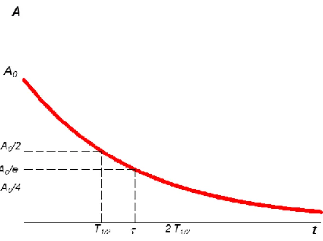
where the parameter is defined as the mean lifetime τ. which is the average time that a nucleus is likely to survive before it decays. Since the activity, A is proportional with the number of atoms present, it follows the same rate of decrease and can be obtained by differentiating the Eq. 1.3; i.e.,

[ ] (Eq. 1.5)

(16)

where A0 is the initial activity at t0 = 0. The SI unit of the activity defined as one

disintegration per second is called Becquerel (Bq). Another unit of activity is the Curie (Ci) which is defined based on the activity of 1 gram of Radium (226Ra) and is equal to 1 Ci = 3.7 x 1010 Bq [Turner J.E., 2007]. Figure 1.1 shows how the activity changes with time following the exponential law of radioactivity.

Figure 1.1: exponential decay of activity.

Therefore, the time trend of a number of parent atoms decreases following the exponential law, while the number of daughter atoms increases follows an exponential trend as shown in figure 1.2.

Figure 1.2: temporal trend of the number of parent atoms and daughter atoms in a radioactive sample.

Some radionuclides may have more than one branches of decay, but independent from the mode of decay, their half-life is the same. For each branch of decay is associated a well-defined probability, represented by the quantity that takes the name of branching ratio. It corresponds to the fraction of particles that decay according to a certain decay

(17)

mode, compared to the total number of particles of the radioactive sample. The branching ratio is a very important property in the study of decays, because for each transition is released a finite amount of energy which is characteristic of the specific branch.

Through the detection of energies associated with the various processes of transition is possible to construct the overall energy spectrum, which allow to identify the type of decay occurred and the elements that produced them, could then go up to the likely progenitor nucleus. The radioactive decay often occurs in a series, or decay chain, in which the generated nuclides are radioactive; the chain ends at the moment when it reaches a stable nuclide. Each of the possible decays is characterized by the decay constant λ1, λ2, …,

λi that expresses the probability that the specific process takes place in the unit of time. The

result is that the overall system will be subject to decay with a total probability connected to constant λt equal to the sum of the different decay constants, i.e.

(Eq. 1.7)

In a closed system, starting from a given quantity of parent atoms, the number of daughter nuclides grows gradually until the moment in which the equilibrium is established within the decay chain. The condition of equilibrium is reached at the time in which the activities of all radionuclides of the decay chain are the equal:

(Eq. 1.8)

This means that the number of daughter nuclides created in the unit of time corresponds exactly to the number of parent nuclides that decay per unit of time: in the case of a series this denotes that the unstable transition will decay with the same rate with which they are produced.

(18)

Figure 1.3: qualitative representation of the secular equilibrium concept. The atoms of 238_{U subject to decay are} represented as a fluid which is poured into the container of 234_{Th. In secular equilibrium conditions the outgoing flow} from the container of 234_{Th, corresponding to the number of atoms of}234_{Th subject to decay, will be equal to the} incoming flow, corresponding to the number of atoms of 234_{Th produced by the decay of}238_{U. If the decay chain of}238_U is in secular equilibrium in its entirety, equality between the incoming and the out coming flow is valid for every element in the chain.

In this way the measurement of the concentration of one of the daughter nuclide can be used to estimate the concentration of any of the other elements belonging to the decay series, and in particular that of the parent nucleus. Inside a decay chain is possible to have a state of disequilibrium: this occurs when the parent nuclide of the chain has a half-life less than those of its progenies, and then disappears while the rest of the chain is active, or in the case in which the chain is broken, that is, when one of the daughter is separated and isolated from the chain.

1.2 The statistical nature of radioactive decay

The process of radioactive decay is a statistical phenomenon. Each disintegration that occurs during a radioactive decay is completely independent from the others, and the time interval between one decay and the next is not constant. For a high number of atoms of a given radionuclide which decay randomly, the frequency of radioactive decay is given by the Poisson distribution: if we denote with n the average rate of decay, with P the probability that a certain number of nuclei n decay at unit of time is given by:

(19)

For a Poisson distribution, the variance σ2 is equal to the mean value of the distribution, where σ is the standard deviation. By increasing the average value of Poisson distribution tends to the Gaussian distribution, ideally for an infinite mean value the two distributions coincide. In this limit the distance of 1σ from the mean value expresses the confidence to find 68.3% of measures with respect to the total, the 95.5% within 2σ and 99.7% within 3σ. In figure 1.4 are represented three Poisson distributions having different average value.

Figure 1.4: example of three Poisson distributions with mean value equal to 1, 5 and 10. It is observed that as average value increase, the Poisson distribution is close to Gauss ones.

If N is the number of decay events recorded at the time t, then the standard deviation in the units of counts is given by:

√ (Eq. 1.10)

where N is the expectation value of the number of counts (i.e., the average value of count assessed by carrying out a certain number of measures).

The relative standard deviation is expressed as:

√ (Eq. 1.11)

By applying the propagation law of errors, for a rate of counts n = N / t it is obtained the standard deviation i.e.,

(20)

√ √ (Eq. 1.12)

therefore the relative standard deviation is:

√ (Eq. 1.13)

From equations above it can be observed that the accuracy of a radiometric measurement can be increased by increasing the number of counts N. This can be achieved by using an instrumentation more sensitive and efficient, improving the geometry of the measurement, or for a longer acquisition time.

1.3 Radioactive decay and decay modes

In nature there are stable nuclei until the lead, around which exists a zone of unstable nuclei, or radioactive, which spontaneously decay into neighbors nuclei with the emission of particles and energy. The stability of a nucleus is determined by its binding energy Eb, which corresponds to the energy required to split the nucleus into individual

protons and neutrons, bringing them to a distance for which there is no strong nuclear interaction between them. This energy depends on the number of protons in relation to the number of neutrons: if the number of neutrons differ a lot of from the number of protons the nucleus is unstable. We can define the binding energy per nucleon, ε, as ratio between the binding energy of nucleus and its mass number:

(Eq. 1.14)

The binding energy per nucleon represents the amount of energy required to split a nucleon (proton or neutron) at a nucleus of mass A.

(21)

Figure 1.5: binding energy per nucleon of common isotopes.

From figure 1.5 it can be seen that ε increase with A, up to A < 60: in correspondence of the iron reaches a maximum equal to 8.79 MeV, then decreases slowly. This decrease in binding energy beyond iron is due to the fact that, as a nucleus gets bigger, the ability of the strong force to counteract the electrostatic repulsion between protons becomes weaker. Elements heavier than these isotopes can yield energy by nuclear fission; lighter isotopes can yield energy by fusion.

The stability of the atoms is determined by the interactions in which its constituents are subject. The increase of Z also increases the repulsive forces of electrical nature between the protons: the nuclear stability is preserved by increasing progressively the number of neutrons, so as to balance the increase of repulsion and prevent decay of the nucleus (Figure 1.6).

(22)

Figure 1.6: representation of the stable nuclei, marked with green squares, as a function of the atomic number Z. The stable nuclei are arranged on the straight line Z = N for values of Z less than 20; for Z > 20, the stability curve towards the axis N, highlighting the greater stability of the nuclei with a number of neutrons greater than the number of protons.

The energies of stable nuclei are lower than unstable nuclei. If we report the energy associated with various nuclei in three dimensional, we find that the permanent ones form a valley, so-called valley of stability (Figure 1.7).

Figure 1.7: three dimensional representation of valley of stability.

The unstable nuclei are located far away from the bottom of the valley; are placed at one of the two sides of the valley depending on whether their instability is generated by

(23)

an excess of neutrons or by an excess of protons. The achievement of a more stable configuration is obtained through two possible types of decay involving the emission of particles: α and β decay. The instability of a nucleus can be caused not only by the overabundance of a type of nucleon, but also by an excess of energy that the nucleon possesses when it is an excited level: in this case there is a third type of decay that causes only the emission of the surplus of energy in the form of electromagnetic radiation, i.e., γ decay.

1.3.1 Alpha decay

The alpha decay occurs in accordance with the conservation law of mass/energy through the emission from the nucleus of an element with high atomic number (Z > 83) of a particle, called alpha particle, consisting in two protons and two neutrons (helium nucleus). There are no α emitters with A < 146 and this can be explained by analyzing the trend of the binding energy per nucleon as a function of the mass number. A nuclear system gains in binding energy emitting α only if it is located beyond the maximum of the curve of figure 1.5, since in this region ε increases with decreasing of the value A. The emission of an alpha particle from the initial nucleus leads to the reduction of mass with four units and two units of charge on the final nucleus as can be seen in the following schematic decay process:

_{(Eq. 1.15)}

The process takes place only for those nuclei in which Q = MX - MY - mα > 0. Between the

initial nucleus and the final products of the decay is exchanged a fixed amount of energy Q, divided among the decay products in such way which is in respect with the conservation of energy and the preservation of the moment. Since this is a decay in two bodies, the energy of the particle α is fixed in the terms of masses of the nuclei. Because the nucleus that accompanies the particle α is much heavier, with a good approximation we can consider that the value Q of the reaction corresponds to the kinetic energy of α emission. The kinetic energies involved are in the order of some MeV.

The emission of an α particle can leave the parent nucleus directly to the ground state of the daughter or leaving the daughter product in an excited states. The final

(24)

daughter nuclide can reach the ground state by releasing the energy through the emission of electromagnetic radiation of γ type. [Cember H., and Johnson T.E., 2009], [Das A.,

and Ferbel T., 2003].

Figure 1.8: schematic representation of decay and - decay of 227_Th.

The energy spectrum resulting from decay is a discrete type: the various lines correspond to the transitions which can occur between the various excited levels of the daughter nucleus.

(25)

Since, α decay has a discrete spectrum, it is possible to conduct α spectrometry measurements thanks to which, on the basis of α emission energy, one can identify the type of atomic species subject to the process of decay.

1.3.2 Beta decay

The β decay corresponds to a transition along an isobar line, which is characterized by a constant value of the mass number A. What occurs is the transformation of neutrons into protons in the case of nuclei with excess of neutrons (decay β-), or on the opposite side of the valley of stability, the transformation of protons into neutrons for nuclei with excess of protons (decay β+ or electron capture).

Figure 1.10: schematic representation of β-_{decay; β}−_{(on the left) and β}+ _{(on the right).}

In the simplest beta-decay process, a free neutron decays into proton emitting an electron and an antineutrino:

(Eq. 1.16)

The process is possible because Q = mn - mp - me = 0.78 MeV (> 0).

The β- decay of a nucleus is substantially the same process, where the energy released varies depending on the binding energies of protons and neutrons in the nucleus, which determine the Q value of the reaction. The transformation that is observed is of the type:

(Eq. 1.17)

The existence of antineutrino e as a product of β- decay was inferred from the

observation of the energy spectrum of electrons produced in the decay. The electronic spectrum, in difference with α spectrum is not discrete but continuous: the kinetic energy extends from a minimum value equal to zero to a maximum value equal to Tmax = MX - MY

(26)

- me. The conservation of energy of angular momentum and charge, respectively require

that the decay is accompanied by a particle with rest mass very small, half-integer spin and neutral charge, particle corresponds precisely to the anti-neutrino. Nuclei that decay in β- decay mode have mean lifetimes between 10-3 and 1023 s, much longer than those of an electromagnetic decay process.

It’s quite unusual that a β transition occurs directly from a ground state of the parent nucleus to the ground state of the daughter nucleus, but in general the state of arrival is an excited state of the daughter nucleus and a β-γ decay occurs. The gamma radiation is released when the daughter nucleus in the excited state is de-energized and reaches the ground state through one or more transitions.

In figure 1.11 is shown the schematic representation decay for 137Cs into 137Ba: it may be affected through pure β- decay to the ground state with a probability of 5.4 % or through a β-γ decay with a probability of 94.6 %.

Figure 1.11: schematic representation decay for 137_Cs.

The β+ decay corresponds to a transformation within a nucleus of a proton into a neutron, accompanied by the release of a positron and an electron neutrino:

(Eq. 1.18)

In this case, there is no a reaction equivalent to the decay of the free neutron described for the β- decay, since the free proton is stable. This is due to the fact that the reaction p → n + e + + νe is prohibited by the conservation of energy, being its value Q negative. But if it is

in the presence of a nucleus, could happen that the neutron is more tied with proton (Q = MX - MY – me > 0), and therefore in this case the reaction can take place. Since the β+

decay, similar to the β-, is a three-body decay, the energy spectrum of the positron is a continuous spectrum. The positrons have a rather short mean lifetime: they are strongly slowed down the passage on the subject, and then annihilate with electrons present in the medium in which they move. From annihilation two photons are produced, each with

(27)

energy Eγ = 0.511 MeV, equal to the rest mass of the electron. From the conservation of

the momentum these photons are emitted in opposite directions.

A different physical process in competition with the β+ decay is electron capture:

(Eq. 1.19)

Therefore electron capture corresponds to a transformation of the type:

(Eq. 1.20)

There is a finite probability of finding an electron in the atomic shell of the nucleus, in particular those of the lower shell, the shell K. Since an electron capture leaves a vacation in the K shell, the electrons perform a cascade to fill emitting of X-ray characteristic. The X-ray emission can be easily followed by other emissions due to the electronic cascade that is generated to fill the gap that moves progressively from the inner electronic shell in the outer ones.

Figure 1.12: schematic representation of electron capture process.

Sometimes the released energy is converted in the production of a photon: it may happen that it is transferred to a third electron, the outermost shell, which is able to reach the level of vacuum. This process is called Auger effect. The Auger electrons are monoenergetic, and usually have low energy, as they are expelled from the atomic shell for which the binding energies are weak.

1.3.3 Gamma decay

The γ decay, unlike α and β decays, doesn’t change neither the atomic mass number A or the charge Z of a nucleus, but involves the dissipation, in the form of electromagnetic radiation, of excess of energy of the excited nucleus. The nucleus possesses similarly to

(28)

atoms energetic levels spaced by bands of forbidden energies: when a nucleus is located in an excited state emits electromagnetic radiation in order to achieve a state of lower energy, hence more stable. Therefore the energy of gamma radiation is well-defined and equal to the difference in energy between the nuclear levels involved in the transition. The γ decay processes are like this:

(Eq. 1.21)

They are qualitatively similar to atomic de-excitation, with an important difference in which the energies involved are of the order of MeV and not of eV. For gamma radiation is defined conventionally as that part of the electromagnetic spectrum that is associated with energy greater than 40 keV. As all electromagnetic waves traveling at the speed of light c, has a discrete energy E, a frequency ν and a wavelength λ, related by the following relationship:

E = (Eq. 1.22)

where h = constant of Planck, equal to 6.626 × 10−34Js and c = speed of light in vacuum, equal to 2.998 · 108 m/s.

The radiation γ usually accompanies an alpha or beta radiation. After emitting α or β, the nucleus is still excited because its protons and neutrons have not yet reached a new equilibrium, and consequently the nucleus is released quickly the surplus energy by emitting electromagnetic radiation. Since the γ radiation due to transitions between energy levels nuclear, it is obviously characteristic of the nucleus that produces it. The energy spectrum generated by a transmitter γ is discrete because it is composed of many energetic levels that make possible the nuclear transitions.

1.4 Sources of radioactivity

We are exposed to environmental radiation from different sources [Klement A.W.,

1982][NCRP Report No.45, 1975]. The origin of radioactivity in the environment can be

(29)

Mostly the naturally occurring radiation arises from terrestrial radioactive nuclides that are widely distributed in the earth’s crust and extra-terrestrial sources arising from cosmic ray

[UNSCEAR 2000]. Also from human activities arise some other sources concerned with

the use of radiation and radioactive materials from which releases of radionuclides into the environment may occur [Eisenbud M., and Gesell T., 1997].

1.4.1 Cosmic radiation

The result of work undertook by Victor Hess between years 1911 and 1913, has explained that there was a radiation penetrating earth’s atmosphere and originating from outside the earth, who gave the radiation the name "cosmic rays". Cosmic radiation comes from both the primary energetic protons and alpha particles of extraterrestrial origin that strike the earth’s atmosphere and the secondary particles or cosmogenic radionuclides which are continuously generated by bombardment of stable nuclides in the atmosphere from these cosmic rays. The primary cosmic rays are those who have not yet any kind of interaction with the present matter in the Earth's atmosphere. They mainly consist of protons and alpha particles, and a small part by heavier nuclei. So the primary cosmic ray composition is very heterogeneous including (about 98% in total, of which 87% consists of hydrogen, 12% of helium and 1% of heavy nuclei), with a small contribution of electrons and positrons (2%) [Bartlett D. T., 2004].

Penetration of cosmic rays depends on several factors, mention here the Earth’s magnetic field and the attenuation caused by the atmosphere, thus only a part of the cosmic radiation incident reaches the earth’s surface, irradiating all living things in continuously way, including human beings. The collision of cosmic radiation particles with atoms in the atmosphere, causes ionization and losing gradually of their energy. The process of energy loss occurs through elastic and inelastic collisions with atomic nuclei, generating a cascade of secondary radiation, as shown in figure 1.13. This secondary radiation includes neutral and charged pi mesons (πo and π+/-), and anti-protons and anti-neutrons (p and n), heavy mesons (K) and hyperons (Y).

(30)

Figure 1.13: representation of the reactions involved in the interaction of particles of primary cosmic rays with the atmosphere, giving rise to secondary cosmic rays.

The cosmic ray flux that reaches at the Earth varies greatly depending on the geomagnetic latitude and at the sea level, consists mainly of muons, electrons and small percentage of neutrons and protons. Muons are the most penetrating components and in spectroscopy is the major source of noise due to cosmic rays.By the interaction of cosmic rays with atoms of the atmosphere through the processes of spallation or neutron capture, we have the production of cosmogenic radionuclides. The spallation is a nuclear reaction in which a nucleus splits into lighter nuclei to collide with a high-energy neutron or a charged particle. In the reaction also produces secondary neutrons which can then give rise to processes of neutron capture. Radionuclides of this nature that contribute most to natural radioactivity are: 3H, 7Be, 14C.

1.4.2 Primordial radionuclides

The primordial radionuclides which are of terrestrial origin, also called terrestrial radionuclides, have been present when the Earth formed about 4.5 billion years ago. These radionuclides have very long half-lives comparable to the age of the earth and are found around the globe in sedimentary and igneous rock. Therefore these radionuclides can migrate from rocks into soil, water and air too. The main primordial radionuclides include the series of radionuclides produced when uranium and thorium decay, as well as 40K and

(31)

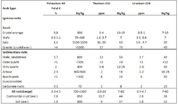
In the Table 1.1 are shown ranges and averages concentrations of 238U, 232Th, and

40_{K in typical rocks and soils [Eisenbud M., and Gesell T., 1997], [IAEA TRS No.419,} 2003].

Table 1.1: ranges and averages of the concentrations of 238_U,232_{Th, and}40_{K in typical rocks and soils.}

The average abundances of the continental upper crust in the world for 238U, 232Th and 40K are respectively 2.7 ppm1, 10.5 ppm and 2.3% [Rudnick R.L., and Gao S., 2003].

Potassium

The 40K is a naturally occurring radioactive isotope of potassium and comprises a very small fraction (about 0.012%) of naturally occurring potassium. Due to the ratio between the abundance of 40K and the total abundance of potassium is fixed, the detection of gamma emission of 40K can be used to estimate the amount of potassium present in the environment. The half-life of 40K is 1.3 billion years, and it decays to 40Ca by emitting a beta particle (89% of the time) with no attendant gamma radiation and to the gas 40Ar by electron capture (11% of the time) with emission of a 1460.86 keV gamma ray.

1_{According to} _{[IAEA TECDOC No.1363, 2003] conversion of radioelement concentration to specific} activity for 1% K = 313 Bq/kg; 1 ppm U = 12.35 Bq/kg and 1 ppm Th = 4.06 Bq/kg. NOTE: These coefficients are calculated for natural isotopic abundances of 99.2745% for 238_{U, 100 % of}232_{Th and 0.0118} % of 40_K.

(32)

Figure 1.14: potassium decay modes.

Uranium

Uranium is found in nature in three different isotopes as 238U (99.2739–99.2752%),

235_{U (0.7198–0.7202%), and a very small amount of}234_{U (0.0050–0.0059%). The}238_U,

otherwise 40K, does not reach the stability with only one decay, but gives rise to a decay chain through which reaches in the stable isotope of 208Pb. Not all of the series nuclides emit gamma radiation, therefore the detection of uranium depends on the gamma rays emitted by some decay products. The most important gamma rays for 238U are those with energy equal to 610 keV, 1120 keV and 1740 keV originated by transition of 214Bi. The half-life of 238U is 4.47 ·109 years.

(33)

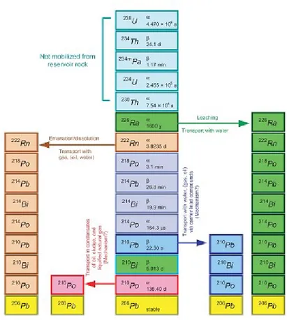
Figure 1.15: uranium decay chain.

Thorium

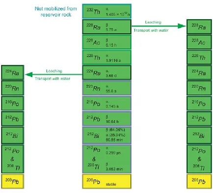
The only constituent of natural thorium is 232Th with a half-life of 1, 39•1010 years. Further there are shorter half-life thorium isotopes in all three natural decay chains, like:

234_{Th (24.1 d half-life) and}230_{Th (7.54 •10}4_{y half-life) in the}238_{U chain;}228_{Th (1.9 y}

half-life) in the 232Th chain; and 231Th (1.06 d half-life) in the 235U chain.

Similarly to 238U gives rise to a decay chain (Figure 1.15), in which the gamma emissions most important are those produced by the transitions of 208Tl at energies of 580 keV and 2614 keV. The decay chain ends with the stable isotope of 208Pb.

(34)

Figure 1.16: thorium decay chain.

All decay products that are in the chain of uranium (Figure 1.15) and thorium (Figure 1.16) have average half-life shorter than that of the generator elements of the series, therefore if the system that contains these radionuclides is isolated, may develop the condition of secular equilibrium. However, there are factors that can lead to breakage of such condition of equilibrium, such as the relatively long life or the chemical-physical characteristics of the decay products. The disequilibrium is generated when one or more decay products within a series are completely or partially removed or added to the system. The thorium rarely leaves the condition of equilibrium, while for potassium the problem does not exist since it decays directly to a stable isotope. Instead in the case of uranium should be considered that its decay chain possesses the rings particularly weak which can lead to breakage of the condition of secular equilibrium, among which the most important is certainly the 222Rn. The 222Rn is a radioactive element with half-life equal to 3.82 days that descends from the alpha decay from 226Ra. It is founded in the gaseous state, therefore in the presence of groundwater or splits can diffuse and reach the surface.

The concentration of radon in the air depends on many factors and can depending on the type of geographic and weather conditions (humidity, rain, snow, day-night, etc.) vary strongly. Radon is also emanating from building materials, which in general contain a certain amount of 226Ra. A significant example is given by the materials of volcanic origin,

(35)

such as tuff. The existence of 226Ra in concrete and plaster, among other very porous materials, contributes to the presence of 222Rn inside buildings. In figure 1.17 and figure

1.18 are highlighted the possible areas in which the condition of secular equilibrium is

broken [IAEA, TRS No.34, 2003].

The disequilibrium in the decay chain of uranium is an important source of error: the uranium concentration is estimated by studying the decay of 214Bi, which is located in a position of decay chain away from uranium generator of the series. Uranium concentrations are therefore defined as concentrations of uranium equivalent, to specify that the values are derived in condition of a secular equilibrium. For the same reason, is evaluated the thorium in indirect mode, by using in this case also the unit of equivalent concentration, although the number of decay of thorium can be considered almost in equilibrium.

Figure 1.17: decay chain of 238_{U where are highlighted the possible points in which the condition of secular equilibrium} is broken.

(36)

Figure 1.18: decay chain of 232_{Th where are highlighted the possible points in which the condition of personal} equilibrium is broken.

1.4.3 Man-made radionuclides

In the environment around us there are many radioisotopes of artificial origin. They come from testing nuclear weapons, from the escape of radioactive material from nuclear power plants, waste from fission released into the environment, the use of certain industrial equipment, from research activity, etc.. The main radioactive elements of anthropogenic origin are: 137Cs, 239Pu, 90Sr, 60Co.

The 137Cs is a radioactive isotope of cesium which is mainly generated as a product of nuclear fission. It has a half-life of 30.07 years and undergoes β- decays into a metastable isotope of 137Ba in 94.6 % of cases, while the remaining 5.4% of the population decays directly on the ground state of 137Ba through a pure decay β-. The 137Cs is water-soluble and very toxic. Detectable quantities of man-made radionuclides are widely distributed in the atmosphere, particularly as a result of nuclear weapons testing and the accident of Chernobyl reactor in 1986.

The concentration of 137Cs in a determined site depends on the environmental conditions during the deposition and dynamics of sedimentation. The 239Pu together with

(37)

235_{U is the main fissile isotope used in the nuclear industry and has a half-life of 24.11}

years. It is normally produced in nuclear reactors exposing 238U to a neutron flux. This is transformed into 239U that undergoes two rapid decays β, transforming first in 239Np and subsequently in 239Pu. After exposure the 239Pu formedis mixed with a residual quantity of

238_{U and traces of other isotopes of uranium, for so is subjected to a purification treatment}

that occurs primarily via chemical.

The 60Co is a radioactive isotope of cobalt, and has a half-life of 5.27 years. It is produced artificially by neutron activation of 59Co. The 60Co undergoes β- decays into 60Ni, which emits gamma radiation with energy respectively 1.17 and 1.13 MeV. The 60Co is mainly used for sterilization of medical equipment, as radiation source for radiotherapy, for industrial radiography or for research purposes.

The 90Sr is a radioactive isotope of strontium with a half-life of 28.8 years. It undergoes β- decays into 90Y, which in turn undergoes β- decays into 90Zr with a half-life of 64 hours. The 90Sr finds many applications in medicine and industry, in particular in the field of radiotherapy surface of some types of cancer. The decay of 90Sr produces a lot of heat and given that 90Sr is cheaper than 238Pu, is often used as a heat source in many radioisotope and thermoelectric generators.

(38)

Chapter 2 2. Gamma-ray spectrometry and principles of gamma ray

detectors

The operation of a detector is based on the interaction of photons constituting the incident radiation with the material that constitutes the detector itself. The gamma radiation interacts with matter via three main processes: the photoelectric effect, Compton scattering and pair production. Thanks to these processes, all or part of the energy possessed by the radiation is transferred to the mass of the detector and then converted into an electrical signal. The basic notions related to the interaction of electromagnetic radiation with matter that we will provide in this chapter will therefore be useful to understand the mechanisms that are at the basis of the generation of a gamma spectrum.

In addition, this chapter will briefly describe the two main types of gamma radiation detectors, i.e. the semiconductor detector and the scintillation, in particular the high-pure germanium detector (HPGe) and a sodium iodide detector activated by thallium NaI(Tl).

2.1 Photoelectric effect

The photoelectric effect is the process by which the energy of incident photon is absorbed by an atom and one of the electrons is released, creating an ion and free electron. During the photoelectric effect the incident photon energy must have higher energy than the binding energy of the inner shell electron. The electron is ejected from its shell, and acquires a kinetic energy equal to:

(Eq. 2.1)

Where is the energy carried by the photon and Eb is the energy required to remove an

electron from the material, which takes the name of binding energy. The quantity Eb

(39)

is spent in the internal electronics collisions. In the case where the binding energy is minimal, the photoelectron emerges with the maximum kinetic energy Emax that is equal to:

(Eq. 2.2)

where Eb is the work function equal to the minimum energy required in order that an

electron can be extracted from the material.

Considering the case in which the maximum energy obtainable from the electron is zero can be go up to the threshold frequency ν0, below which the photoemission process

cannot take place:

(Eq. 2.3)

The photon frequency ν0 is one of that has sufficient energy to remove the electron without

giving any kinetic energy. If the frequency is less than the threshold value of the radiation, regardless of the intensity, will not have enough energy to remove the electron from the material.

The photoelectric effect leaves the atom in an excited state with an excess of energy equal to and a gap in the electronic orbit from which it was released the photoelectron. The gap created following the expulsion of the photoelectrons can be progressively filled by electrons from the outer orbits resulting in a characteristic X-ray emission. Alternatively, the excitation energy can be carried away by the release of other, less tightly bound electrons known as Auger electrons.

Figure 2.1: schematic representation of the photoelectric effect and the subsequent emission of X-ray characteristic.

During photoelectric process the interaction cross section (τ) varies in a complex manner with E and with the Z value of the absorber as follow:

(40)

(Eq. 2.3)

where n and m are numbers that vary in the range from 3 to 5 over the gamma-ray energy region of interest. Probability of photoelectric absorption strongly depends on photon energy and atomic number of an absorber material. While the strong dependence of Z shows that a high-Z material is very effective in the absorption of photons. The strong dependence on the photon energy is the reason why the photoelectric process is significant at low energy of photons, but becomes less dominant at higher energies.

2.2 Compton scattering

The Compton effect is a phenomenon of scattering representable as a collision between the incident gamma-ray photon and weakly bound or free electron in the absorbing material.

Figure 2.2: schematic representation of the scattering between a photon and a free electron.

In the collision part of the energy of the photon is transferred to the electron by the expression:

_[

] (Eq. 2.4)

where me is indicated the electron mass and θ the angle formed by the radiation deflected

respect to the direction of incidence. The transfer of energy can be formulated also according to variation of the photon wavelength.

(41)

(Eq. 2.5)

where λc is the Compton wavelength defined by:

(Eq. 2.6)

The energy acquired by the electron depends on the direction in which the incident photon is deflected: if θ = 0◦, or if the direction of deviation of the photon coincides with the direction of incidence, Ee is equal to 0, and therefore no energy is transferred to the

electron. The photon maintains its initial energy, giving rise to a process of elastic scattering, known as Rayleigh scattering. In the case diametrically opposite, in which the photon is scattered backwards at an angle θ = 180◦, the energy acquired by the electron is the possible maximum but less than the energy carried by the incident photon. For each possible scattering angle the percentage of energy transferred to the electron is always less than 100%.

In the Compton scattering process the probability depends strongly on the number of electrons per unit mass of the interacting material. It also depends on the incoming gamma-ray energy as function of [Lilley J., 2001], [Gilmore G.R., 2008]. Compton scattering is the dominant interaction process for gamma-ray energies ranging from 0.1 to 10 MeV [Das A., and Ferbel T., 2003]. Another interaction mechanism, known as ‘pair production’ becomes more significant at the higher energy.

2.3 Pair production

The pair production occurs when a photon of high energy loses all its energy in the interaction with an atomic nucleus, giving rise to an electron-positron pair. This phenomenon take place if the photon energy is greater than a threshold value of 1022 keV, equal to the sum of the rest mass produced by particles, therefore equal to twice the mass of the electron.

(42)

Figure 2.3: schematic of the Compton scattering process.

In the pair production the energy that is transferred to the nucleus is negligible, being much more massive respect to the particles produced. Thus the total relativistic energy is given by (Eq. 2.7):

(Eq. 2.7)

where K- and K+ indicate the kinetic energy of electron and positron respectively. The

positron is produced with energy slightly higher than the electron due to the Coulomb interaction of the pair with the positively charged nucleus produces an acceleration of the positron and electron deceleration.

After creation of electron - positron pair, they can traverse the medium, losing their kinetic energy by collisions with electrons in the surrounding material through ionization, excitation and/or bremsstrahlung. When the energy of the positron reaches values close to the thermal energy, it annihilates with an electron surrounding releasing the two annihilation photons of 511 keV. The energy (expressed in keV) which is absorbed by the detector following the pair production will be equal to:

(Eq. 2.8)

2.4 The probability interaction and correction of gamma radiation

The probability that a photon interacts with matter is expressed in terms of the cross section σ (m2), which represents qualitatively the product of the area in which takes place

(43)

the total-area for the probability that the interaction occurs the same. The cross section depends both from energy Eγ of photons and the composition of the surrounding matter.

In the figure 2.4 is shown the trend of the cross section as a function of energy Eγ.

From the graph it is clear that the photoelectric effect is the dominant phenomenon for energies below 100 keV: in this energy range are observed evident peaks in the form of the cross section, which are found in correspondence of the binding energies of the different atomic shell. Compton scattering dominates the events of medium energy, while the pair production is possible only for energies above the threshold of 1022 keV.

For the three processes of interaction between radiation and matter is possible to define the trend of the cross section as a function of photon energy Eγ and as a function of

the atomic number Z of the material in which the photons pass through.

For the photoelectric effect its dependence can be approximately expressed by the following relation:

with n = (Eq. 2.9)

The strong dependence from the atomic number indicates that a material with high value of Z is very effective in the absorption of photons. The dependence of the photon energy is a reason why the photoelectric effect is dominant for low energies.

Figure 2.4: cross section for the photoelectric effect, Compton scattering and pair production and the total cross section for an atom of Lead as a function of the photon energy.