Transverse Gravitational Theories

(1)

Transverse Gravitational Theories

1 Introduccion

1.1 Equivalence principles, metric theories and universal cou-pling

The Principle of Equivalence, from the beginning, has played an im-portant role in the development of gravitational theories: Newton him-self dedicated a detailed discussion of it in the opening paragraphs of his “Philosophiae naturalis principia matematica”. To Newton, the Principle of Equivalence demanded that the “mass” of any body, namely the property of any body (inertia) that regulates its response to an applied force, be equal to its “weight”, that property that regulates its response to gravitation. Bondi in 1957 coined the terms “inertial mass” (mi) and “passive

gravita-tional mass” (mp) to refer to these quantities, so that Newton’s second law

and the law of gravitation take the form

F = mia F = mpg.

The Principle of Equivalence can then be succinctly stated saying that

For any body mi = mp.

with a more precise statement it can be expressed by saying that

If an uncharged test body is placed at an initial event in spacetime and given an initial velocity there, then its subsequent trajectory will be independent of its internal structure and composition.

By “uncharged test body” we mean an electrically neutral body with negli-gible self-gravitational energy.

Today Newton’s Equivalence Principle is generally referred to as the Weak Equivalence Principle (WEP).

According to the WEP, if all bodies fall with the same acceleration in an external gravitational field, then, to an observer in a freely falling elevator in the same gravitational field, the bodies should be unaccelerated (assuming that small effects due to inhomogeneities in the gravitational field can be made as small as desired by working in a sufficiently small elevator). Thus, insofar as their mechanical motion are concerned, the bodies will behave as if gravity were absent.

It was Einstein who added the key element to the WEP that revealed the path to General Relativity. Going one step further, he proposed that not only should mechanical laws behave in such an elevator as if gravity were absent, but so should all the laws of physics, including for example the

(4)

laws of electrodynamics: that is, “we [...] assume the complete physical equivalence of a gravitational ﬁeld and a corresponding acceleration of the reference system” (Einstein 1907). Thus being at rest on the surface of the Earth is equivalent to being inside a spaceship (far from any sources of grav-ity) that is being accelerated by its engines. From this principle, Einstein deduced that free-fall is actually inertial motion. By contrast, in Newtonian mechanics, gravity is assumed to be a force, so that a person at rest on the surface of a (non-rotating) massive object is in an inertial frame of reference. Now this is called the Einstein Equivalence Principle (EEP), and can be expressed with the statement that

The Weak Equivalence Principle is valid and the outcome of any local non-gravitational experiment in a freely falling laboratory is independent of the velocity of the laboratory and its location in spacetime.

By “local non-gravitational experiment” we mean any experiment performed in a shielded freely falling laboratory with negligible self-gravitational eﬀects. The EEP is essentially composed by three diﬀerent parts: WEP, Local Posi-tion Invariance (LPI) i.e. invariance under locaPosi-tion change of the laboratory, and Local Lorentz Invariance (LLI) i.e. invariance under velocity change of the laboratory.

Today a third Equivalence Principle exists, which is much more re-strictive than Einstein’s formulation: the Strong Equivalence Principle (SEP) states that

The gravitational motion of a small test body depends only on its initial position in spacetime and velocity, and not on its constitution. The outcome of any local experiment (gravitational or not) in a freely falling laboratory is independent of the velocity of the laboratory and its location in spacetime.

The first part is a version of the WEP that applies to objects that exert a gravitational force on themselves, while the second part is the EEP re-stated to allow gravitational experiments and self-gravitating bodies. Some powerful consequences [1] of the SEP are that the gravitational con-stant G must be the same everywhere in the universe, and that a fifth force beyond the known ones is not allowed. Anyway, some physicists have criti-cized the differences made between the EEP and the SEP because there is no universally accepted way to distinguish gravitational from non-gravitational experiments.

(5)

Today, in most gravitational theories, gravitation is a curved-spacetime phenomenon, i.e. must satisfy the postulates of “metric theories” which state that

Spacetime is endowed with a metric gµν. The world lines of test bodies are

geodesics of that metric. In local freely falling frames, called local Lorentz frames, the non-gravitational laws of physics are those of special relativity.

It is possible to argue that if a theory satisﬁes the EEP, it is a metric theory [1].

Metric theories are equivalent to those characterized by the so called uni-versal coupling, that is the property that all non-gravitational ﬁeld should couple in the same manner to a single gravitational ﬁeld. It’s only a matter of choosing to consider the metric gµνas a property of spacetime itself rather

than as a field over a flat spacetime. Thus metric theories can differ from each other only in the number and type of additional gravitational fields they introduce and in the field equations that determine their structure and evolution. There may be other gravitational fields besides the metric which contribute to the curvature of spacetime; nevertheless, once determined the evolution of the metric, the only field that couples directly to matter is the metric itself.

1.2 Schiﬀ ’s conjecture [1]

The three parts of EEP are so diﬀerent in their empirical consequences that it is tempting to regard them as independent theoretical principles. Anyway, in 1960 Leonard Schiﬀ conjectured that any complete, self-consistent

theory that embodies WEP necessarily embodies EEP. By a complete

self-consistent theory we mean a theory capable of predicting the results of any experiment of interest, giving the same result through whichever method is used.

A rigorous proof of the conjecture could give much stricter bounds to the violation of EEP. Anyway, so far only “plausibility” arguments have been found. One of the most elegant of these, for instance, assumes the conser-vation of energy:

Let’s consider an idealized composite body made up of structureless test particles bounded by some non-gravitational force, which moves suﬃciently slowly in a weak, static gravitational ﬁeld to describe the motion in a quasi-Newtonian form (so that second order terms∼ v4, U2 can be neglected). If

(6)

to be regarded as point-like, we can assume that the conserved energy func-tion has the general form

E = MRc2− MRU (x) +

1 2MRv

2_{+ o(v}2_{, U ).}

If we assume EEP violations, the speed of light could depend on the presence of gravity, so we don’t set c = 1. The rest energy can be written as

MRc2= M0c2− EB(x, v)

where M0 is the sum of the rest masses and EB is the binding energy

that, expanded in powers of U and v2, can be written as

EB(x, v) = EB0+δmijpUij(x)− 1 2δm ij Ivivj ( Uij(x)≡ ∫ d4xρ(x− x ′₎ i(x− x′)j |x − x′_|3 ) .

It can be shown that δmijp and δmij_I (called anomalous passive and

iner-tial mass tensors, which depend upon the internal structure of the body) are possible terms that give rise to EEP violation, since a freely falling observer, detecting the binding energy of the system, could detect the eﬀects of his location and velocity. Let’s prove that they give rise also to WEP violation, through a “gedanken experiment”:

We start from n free particles of mass m0 at rest at x = h; their conserved

energy is

nm0(c2− U(h)).

We form a bound state and keep the energy released EB(h, 0) in a reservoir

of free particles of mass m0. Now the conserved energies of the bound state

and the reservoir are respectively

[nm0c2− EB(h, 0)][1− U(h)/c2] and EB(h, 0)[1− U(h)/c2].

We let the stored particles and the bound system freely fall, with accel-erations g =∇U and a = g + δa respectively, until x = 0. Here we bring the systems at rest and put into the reservoir the kinetic energies collected

−[nm0− EB(0, v)/c2]a· h − δmij_Igihj and − EB(h, 0)g· h/c2

(some kinematic identities have been used to substitute v). From the reservoir, that now has energy

EB(h, 0)[1− U(0)/c2]− E0Bg· h/c2− (nm0− E0B/c2)a· h − δm ij Igihj

(7)

we extract enough energy (EB(0, 0)[1− U(0)/c2]) to deassemble the

bound system, and enough energy (−nm0g· h) to carry the n particles back

at x = h. The cycle is closed, and if energy is conserved the reservoir should be empty. This means that we must have

EB(h, 0)− EB(0, 0)− (nm0− EB0/c2)δa· h − δm ij Igihj = 0. Since EB(h, 0)− EB(0, 0) = δmijp∇Uij · h we get ai = gi+ δmjkp MR ∂iUjk − δmij_I MR gj.

So, since the WEP would give ai= gi, WEP is violated unless

δmijp = δmij_I = 0. Schiﬀ’s conjecture, under the assumptions made, is

proved. Anyway, the whole argument is valid only in the non-relativistic limit.

(8)

2 Transverse mass-less theories

2.1 What are Transverse Theories?

Einstein’s General Relativity has the property to be invariant under a general diﬀeomorphism in the coordinates (Diﬀ invariance). This property is manifest if we get to Einstein’s equations starting from the variational principle of the Hilbert action

S = ∫ d4x√−g [ − 1 2k2R + Lm ] (2.1.1) since d4x√−g is a scalar for generic diﬀeomorphic transformations.

Here we have deﬁned

k2≡ M_P−2 ≡ 8πG. (2.1.2)

Anyway, it is maybe not well known that, four years after writing down the equations of General Relativity, Einstein also proposed a different set of equations, which are the traceless part of the ones of General Relativity. This different set of equations comes out from those theories which are now commonly called “unimodular theories” [3], in which the determinant of the metric g is fixed. Although Einstein never talks about an action principle (since he was actually interested only in the equations of motion), if we work in the variational formalism, unimodular theories constrain the allowed unimodular variations δugαβ to be such that

δug = 0 (2.1.3)

or equivalently

gµνδugµν = 0. (2.1.4)

This means that the unimodular variation can be expressed in terms of an unconstrained variation as

δugαβ = δgαβ−1 4g

αβ_g

µνδgµν (2.1.5)

so that any variation of an action can be expressed as

δS = δS δgαβδg αβ ₌ δS δgαβ ( δugαβ+1 4g αβ_g µνδgµν ) . (2.1.6)

Eventually, the restricted variation is just the trace-free part of the uncon-strained variation:

δS

= δS −1gαβgµν

δS

(9)

Hence, calculating the restricted variation of the Hilbert action we get the equations Rαβ − 1 4gαβR = k 2(_T αβ− 1 4gαβT ) (2.1.8) which are exactly the second traceless set of equations proposed by Ein-stein.

It seems that this alternative set of equations carry less information than the well known Einstein equations, because the trace has been left out. But Einstein himself realized in 1919 that this unimodular theory is equivalent to General Relativity, with the Cosmological Constant appearing as an in-tegration constant:

If we assume the energy-momentum to be covariantly conserved and using the contracted Bianchi identity ∇νRµν = 1₂∇µR (where ∇ν are covariant

derivatives), deriving by∇β the whole equation we get 1

4∇αR =−

k2

4 ∇αT (2.1.9)

which integrated gives

R + k2T = constant≡ −4Λ. (2.1.10) Finally, if we substitute T in equation (2.1.8) we get exactly Einstein’s Gen-eral Relativity equations:

Rαβ−

1

2gαβR− gαβΛ = k

2_T

αβ. (2.1.11)

Transverse Theories [2] are a bit different from unimodular theories: in Transverse Theories the determinant of the metric g is not fixed (it’s dynamical), so that the variation δgαβ is not restricted by δg = 0. But the action is invariant under transverse diffeomorphisms (TDiff ) in the sense that the gauge symmetry group of the Lagrangian is not the whole group of diffeomorphisms, but only the TDiff group.

The TDiﬀ group is the group of the diﬀeomorphisms that leave the determinant of the metric g unchanged. We have

δg = ggµνδgµν (2.1.12)

where, at the ﬁrst order, for a linear transformation

(10)

we have

δgµν = ξρ∂ρgµν + gρµ∂νξρ+ gρν∂µξρ=∇µξν+∇νξµ (2.1.14)

with ∇µ denoting covariant derivatives. Hence, since invariance under

TDiﬀ means that δg = 0, we must have

δg = ggµν(∇µξν+∇νξµ) = 2g∇µξµ= 0 (2.1.15)

i.e.

∇µξµ= 0. (2.1.16)

Vector ﬁelds inducing TDiﬀ transformations can generically be repre-sented as [4]

ξµ= ϵµνρσ∇νΩρσ (2.1.17)

where ϵµνρσ is the Levi-Civita controvariant tensor and Ωρσ is an

anti-symmetric tensor. Since ϵµνρσ is completely antisymmetric, the contraction with the symmetric term∇µ∇ν implies that

∇µξµ= ϵµνρσ∇µ∇νΩρσ= 0. (2.1.18)

Given a metric gµν, we can split it into

gµν ≡ ηµν+ khµν (2.1.19)

where ηµν is the ﬂat Minkowski metric and k2 ≡ 8πG so that the

devia-tion hµν from the ﬂat metric can be regarded as a tensor ﬁeld of dimension

one.

The former is an exact deﬁnition of hµν, so that the inverse metric can only

be written as a formal power of series

gµν = ηµν− khµν+ k2hµ_ρhνρ− k3hµρhρσhνσ+ O(k4). (2.1.20)

When using the ﬁeld hµν the indexes are always raised and

low-ered by the ﬂat Minkowski metric.

The variation of hµν, at the lowest orders,is given by

(11)

If we consider weak ﬁelds, we can consider only the term proportional to

k−1: at the ﬁrst order we can say that TDiﬀ transformations are those gauge transformations

kδhµν = (∂µξν+ ∂νξµ) (2.1.22)

which satisfy

∂µξµ= 0. (2.1.23)

2.2 Why Transverse Theories?

General Relativity is perfectly consistent as a classical theory, and in-sofar almost every experiment surprisingly agrees with the theoretical pre-dictions. Anyway, two are the main problems Einstein’s theory has to deal with: (i) the difficulties to extend the classical theory to consistent renor-malizable quantum field theories, which have been so successful in describ-ing all the other interactions; (ii) the Cosmological Constant problem: if the cosmological constant is the vacuum energy, why has it such a tiny value Λ = M_D4 ∼ 10−48GeV4 and isn’t it of the order of the cutoff scale

M4

P ∼ 1076GeV4?

Mainly for these reasons General Relativity is not considered the definitive answer for Gravity, and many modifications have been considered (like for instance String Theories). So, one of the possibilities is to modify General Relativity postulating less spacetime symmetry, like in Transverse Theories, which leaves us with more freedom in writing the possible actions. More precisely, two are the main arguments that justify the interest in TDiff the-ories:

• Consistent propagation of a massless spin-2 graviton requires only

TDiﬀ invariance [3] [2] [5]:

In the standard “transverse-traceless gauge”, the ﬁve polarizations ϵµν

of a spin-2 symmetric tensor ﬁeld must satisfy

∂µϵµν = 0 (2.2.1)

ϵµ_µ= 0 (2.2.2)

where ϵµν ≡ ηµνϵµν. Thus, for a mass-less particle with four-momentum

(12)

as ϵ×_µν = e1⊗ e2+ e2⊗ e1 ϵ+_µν = e1⊗ e1− e2⊗ e2 ϵ(1)_µν = k⊗ k ϵ(2)_µν = k⊗ e1+ e1⊗ k ϵ(3)_µν = k⊗ e2+ e2⊗ k. (2.2.3)

We notice that ϵ(1,2,3)µν are all of the form kµξν+ kνξµ with kµξµ= 0.

First, in the mass-less case, we would like to be left with the only two helicity-eigenstate polarizations (which are known to be ϵ+

µν± ϵ×µν). Next,

we have to deal with the inﬁnite degeneration arising from the “little group” problem; the “little group”, which in this case is the group of the transfor-mations that leave the four-momentum (k, 0, 0, k) of a mass-less particle un-changed, has three generators: Iz (rotation around the z-axis) and I0x, I0y

(boost along the x, y-axis plus a rotation around the y, x-axis to “neutralize the aberration” coming from the boost).

Iz unitarily acts in the right way on the standard helicity polarizations

ϵ+_µν ± ϵ×_µν, giving only a phase e±2iθ under rotations of angle θ. But the inﬁnite dimensional unitary representation of the non-compact transforma-tions I0x, I0y lead to the appearance of inﬁnite polarizations for any given

momentum. We would like to solve the problem in a similar way as for the abelian case of Electrodynamics, i.e. through a gauge-invariant principle. The standard helicity polarizations transform under I0x, I0y into the other

three ϵ(1,2,3)µν . Moreover, I0x, I0y leave the trace ϵµµ unchanged, since the

trace is Lorentz-invariant. It is then straightforward to declare equivalent those polarizations which are related to one another by a standard gauge transformation

ϵµν −→ ϵµν − (kµξν + κνξµ) (2.2.4)

which leaves the trace invariant, that is such that

kµξµ= 0.

This way I0xand I0y become only gauge-invariant transformations, and the

three polarizations ϵ(1,2,3)µν become “pure gauge”.

To solve the problem only TDiﬀ invariance is needed.

• In Transverse Theories it is possible to make the coupling of the metric gµν to the vacuum energy Λ as small as desired:

Since TDiﬀ transformations leave the determinant of the metric g invariant,_√

(13)

with an arbitrary function f (g). It means that we could write an action with a term

Sv =

∫

d4xf (g)Λ (2.2.5)

which allows us, playing with the function f (g), to make the coupling between the metric and the vacuum energy arbitrarily small: Λ could even be of the order of M_P4.

2.3 TDiﬀ quadratic Lagrangian

We are going now to analyze the linearized theory.

The most general quadratic Lorentz-invariant local Lagrangian for a free massless symmetric tensor ﬁeld hµν can be written as [2]

L = L0+ c1L1+ c2L2+ c3L3 (2.3.1) where L0 ≡ 1 4∂µh νρ_∂µ_h νρ (2.3.2a) L1 ≡ − 1 2∂µh µν_∂ ρhρν (2.3.2b) L2 ≡ 1 2∂µh∂νh µν _(2.3.2c) L3 ≡ − 1 4∂µh∂ µ_h. _(2.3.2d)

L0 is strictly needed for the propagation of a spin-2 particle.

(14)

δL0 =− 1 22hµνδh µν _(2.3.3a) δL1 = (∂µ∂ρhρν + ∂ν∂ρhρµ)δhµν (2.3.3b) δL2 =− 1 2(∂µ∂νh µν_{δh + ∂} µ∂νhδhµν) (2.3.3c) δL3 = 1 22hδh. (2.3.3d)

For TDiﬀ gauge transformations, (2.1.22) with the constraint (2.1.23), we notice that

δL2= ∂µ∂νhµν∂ρξρ+ ∂µ(∂νh∂νξµ)− ∂νh∂ν∂µξµ= 0 (2.3.4a)

δL3=−2h∂µξµ= 0. (2.3.4b)

So, to have TDiﬀ invariance it’s only necessary that c1 = 1:

δL0+ δL1 =−(∂ρ∂µhρν + ∂ρ∂νhρµ− ∂ρ∂ρhµν)(∂µξν+ ∂νξµ) = 0 (2.3.5) because      (∂ρ∂µhρν− ∂ρ∂ρhµν)∂µξν = ∂ρ[(∂µhρν − ∂ρhµν)∂µξν]− (∂µhνρ− ∂ρhµν)∂ρ∂µξν = 0 ∂ρ∂νhρµ∂µξν = ∂ν(∂ρhµρ∂µξν)− ∂ρhρµ∂µ∂νξν = 0

The most general quadratic TDiﬀ-invariant Lagrangian is then

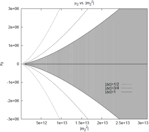
L = 1 4∂µh νρ_∂µ_h νρ− 1 2∂µh µν_∂ ρhρν+ c2 2∂µh∂νh µν₋c3 4∂µh∂ µ_h. _(2.3.6)

(15)

2.4 Dynamical analysis

We will still work in the approximation of a linear theory.

As shown in section (2.2), the quantum theory of Gravitation is not unitary unless the Lagrangian is invariant under TDiﬀ. Actually, we will show that the absence of TDiﬀ symmetry leads to pathologies such as classical insta-bilities or the appearance of ghosts.

Let’s use the “cosmological decomposition” for the ﬁeld hµν in terms of

scalars, vectors and tensors under spatial rotations [6]:

h00=A (2.4.1a)

h0i=∂iB + Vi (2.4.1b)

hij =ψδij + ∂i∂jE + (∂iFj+ ∂jFi) + tij (2.4.1c)

with

∂iFi= ∂iVi= ∂itij = tii= 0. (2.4.2)

With this decomposition, in the generic quadratic Lagrangian (2.3.1), scalars, vectors and tensors decouple from each other; working in momen-tum space [2]:

• The tensor tij only contributes to L0:

Lt=

1 4(∂µt

ij₎2_. _(2.4.3)

• The vectors contribute only to L0 and L1:

Lv = 1 2k 2_(Vi_{− ˙F}i₎2₊1 2(c1− 1)(k 2_Fi_{+ ˙}_Vi₎2_. _(2.4.4)

The momenta conjugated to Vi and Fi are

Πi_V = (c1− 1)(k2Fi+ ˙Vi) (2.4.5a)

Πi_F = k2( ˙Fi− Vi) (2.4.5b)

so that (2.4.4), for c1 ̸= 1, can be rewritten as Lv = 1 2k2Π 2 V + 1 2(c1− 1) Π2_F. (2.4.6)

(16)

The Hamiltonian is given by Hv = 1 2k2(Π i F+k2Vi)2− 1 2(1− c1) [ Πi_V + (1− c1)k2Fi ]2 +1− c1 2 k 4_F2₋1 2k 2_V2_. (2.4.7) Because of the alternating signs, the Hamiltonian is not bounded below, which leads to classical instability: from Hamilton’s equations we have

˙

Πi_F = k2Πi_V (2.4.8a)

˙

Πi_V =−Πi_F (2.4.8b)

which give the general oscillatory solution

|k|Πi

V + iΠiF = Cexp[i(|k|t + ϕ0)], (2.4.9)

while taking the derivative of (2.4.5) with respect to t and using (2.4.8), we have ¨ Vi+ k2Vi=− c1 c1− 1 Πi_F (2.4.10a) ¨ Fi+ k2Fi= c1 c1− 1 Πi_V (2.4.10b)

which, for c1 ̸= 0 are the equations of forced oscillators with asymptotic

solution

Vi+ i|k|Fi ∼ Cc1t (c1− 1)|k|

exp[i(|k|t + ϕ0)]. (2.4.11)

The solution, which grows linearly with time, is the evidence of classical instability.

Classical instability could be avoided setting c1 = 0. But in this case the

vectors Vi and Fi would decouple from each other and Vi would become a ghost, since Lv(c1= 0) = 1 2k 2_(∂ µFi)2− 1 2(∂µV i₎2_. _(2.4.12)

(17)

case

Lv(c1 = 1) =

1 2k

2_(Vi_{− ˙F}i₎2_. _(2.4.13)

The variation with respect to Vi _{gives the constraint}

Vi− ˙Fi= 0 (2.4.14)

which, substituted in (2.4.13), shows that there is no vector dynamics.

• The scalar Lagrangian, with c1 = 1, is given by

Ls= 1 4 [ (∂µA)2− 2k2(∂µB)2+ 3(∂µψ)2− 2k2∂µψ∂µE + k4(∂µE)2 ] − 1 2 [ ( ˙A + k2B)2− k2B˙2− k2ψ2+ 2k4Eψ− k6E2+ 2k2B(ψ˙ − k2E) ] + c2 2 [ ( ˙A− 3 ˙ψ + k2E)( ˙˙ A + k2B)− k2(A− 3ψ + k2E)( ˙B− ψ + k2E) ] − c3 4 [ ∂µ(A− 3ψ + k2E) ]2 . (2.4.15) The variation of B gives the constraint

2ψ = (c2− 1)(A − 3ψ + k2E) = (c2− 1)h (2.4.16)

that, substituted back in (2.4.15), gives the simple expression

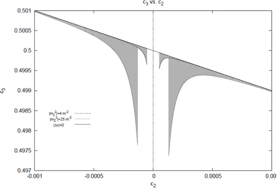
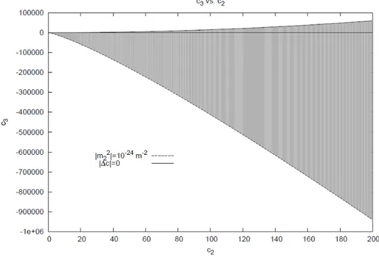
Ls=− ∆c3 4 (∂µh) 2 _(2.4.17) where ∆c3 ≡ c3− 3c2₂− 2c2+ 1 2 . (2.4.18)

Hence, the scalar sector contains a single degree of freedom, proportional to the trace.

Moreover, to avoid ghosts, we must have the condition

∆c3 ≤ 0. (2.4.19)

In the special case where

∆c3= 0 (2.4.20)

the scalar sector disappears, and we are left only with the tensor sector.

(18)

2.5 Non-linear generalizations

The simplest way to generalize TDiff theories is to mix the Hilbert action with general functions of the determinant of the metric: since by definition TDiff transformations leave the determinant unchanged, these functions are also TDiff-invariant.

Hence, a general gravitational TDiﬀ-invariant action could be of the form

S = ∫ d4x ( − 1 2k2 ) ( f1(|g|)R + f2(|g|)gµν∂µg∂νg ) . (2.5.1)

To extend to non-linear theories the study of TDiﬀ-invariance we could even make some particular choices: as seen in the previous section, in general TDiﬀ quadratic theories there is a supplementary scalar degree of freedom, proportional to the trace h. Thus, the idea [7] is to split the metric degrees of freedom into the determinant g and a new metric

ˆ

gµν ≡ |g|−1/4gµν (2.5.2)

with ﬁxed determinant |ˆg| = 1. Under arbitrary diﬀeomorphisms (2.1.13) the new metric transforms as

δˆgµν = ˆ∇µξν+ ˆ∇νξµ−

1

2gˆµν∇ˆρξ

ρ _(2.5.3)

where ˆ∇ denotes covariant derivative with respect to ˆgµν, and the indexes

are raised and lowered by the new metric. Transverse diﬀeomorphisms are deﬁned as those which satisfy

ˆ

∇µξµ= 0. (2.5.4)

But since |ˆg| ≡ 1, we have that ˆΓµµν = ∂ν

√

|ˆg| = 0 so that condition (2.5.4)

reduces to

ˆ

∇µξµ= ∂µξµ+ ˆΓµµνξν = ∂µξµ= 0. (2.5.5)

Hence, under TDiﬀ with the constraint (2.5.4) the metric ˆgµν transforms

as a tensor:

δˆgµν = ˆ∇µξν + ˆ∇νξµ (2.5.6)

and also the determinant g, as expected, transforms as a scalar:

(19)

It can be shown [7] that the only terms which can be constructed from ˆgµν

that behave as tensors are the geometric tensors ˆRµνρσ and its contractions,

so that the most general TDiﬀ-invariant action which contains at most two derivatives of the metric takes the form:

S = ∫ d4x ( −1 2χ 2_(g,_{{ϕ}) ˆ}_{R + L(g,}_{{ϕ}, ˆg} µν) ) (2.5.8) where χ2 is a scalar made out of the matter ﬁelds{ϕ} and the determinant

g.

We thus notice that TDiﬀ-invariant theories can be seen as “unimodular” (i.e. with ﬁxed determinant) scalar-tensor theories, where g plays the role of an additional scalar.

The equations of motion must be calculated through a restricted variation of the metric, since the action is composed of a metric with ﬁxed determinant ˆ g = 1. If we deﬁne ¯ gµν ≡ χ2gˆµν (2.5.9) so that _√ −¯g =√−χ8_{g = χ}_ˆ 4 _(2.5.10)

we can go to the “Einstein frame”: the new action reads

S = ∫ d4x√−¯g [ −1 2R(¯gµν) + 6 χ2 ¯gµν∂µχ∂νχ + 1 χ4L(χ,¯ {ϕ}, ¯gµν) ] . (2.5.11) Anyway, we have to implement the constraint (2.5.10), that can be done through a Lagrange multiplier Λ(x). Hence we have

S = ∫ d4x√−¯g [ −1 2R(¯gµν) + 6 χ2g¯µν∂µχ∂νχ + 1 χ4L(χ,¯ {ϕ}, ¯gµν) ] − ∫ d4x√−¯g 1 χ4Λ + ∫ d4xΛ. (2.5.12)

We note that the invariance under full diﬀeomorphisms which treat ¯gµν

as a metric and χ and Λ as scalars is only broken by the last term. We can show that this term is actually an integration constant, and not a parameter of the Lagrangian.

(20)

If we deﬁne the matter Lagrangian as Lm ≡ √ −¯g [ 6 χ2 ¯gµν∂µχ∂νχ + 1 χ4L(χ,¯ {ϕ}, ¯gµν)− 1 χ4Λ ] + Λ (2.5.13)

the Bianchi identities applied to the pure gravitational part√−¯g1₂R(¯gµν)

give, as in General Relativity, the conservation of the energy-momentum tensor

∇µTµν = 0 (2.5.14)

where the energy-momentum tensor is deﬁned as

Tµν ≡

2

√_−¯gδLm

δ¯gµν. (2.5.15)

On the other hand, since only the last term of (2.5.13) breaks Diﬀ-invariance, the variation of the matter part of the action under a general coordinate transformation is given by

δLm= δLm δχ δχ+ δLm δψ δψ + δLm δΛ δΛ+ √_−¯g 2 Tµνδg µν _{= δΛ = ξ}µ_∂ µΛ. (2.5.16)

If the equations of motion for χ, Λ and ψ are satisﬁed, i.e.

δLm δχ = δLm δψ = δLm δΛ = 0, (2.5.17)

since δgµν =∇µξν +∇νξµ, after partial integration we get ξµ(∂µΛ +

√

−¯g∇ν_T

µν) = 0 (2.5.18)

that is, using (2.5.14),

(21)

2.6 Lorentz covariance and compensators

Usually, tensor densities of weight w are deﬁned in such a way that they get an extra factor of the Jacobian to the power w in the tensorial transformation law. For instance a scalar of weight w transforms as

ϕ′(y) = D(y, x)wϕ(x) (2.6.1) where D(y, x)≡ det ( ∂yµ ∂xν ) . (2.6.2)

A particular scalar density is the determinant of the metric g, which behaves as a scalar density of weight w =−2, that is

g(y) = ( 1 D(y, x) )2 g(x). (2.6.3)

TDiﬀ transformations are actually those transformations with unitary Ja-cobian (D(y, x) = 1).

This means that as long as we assume that TDiﬀ is the basic symmetry of nature, we do not distinguish tensor densities from real tensors.

Now, going back to the study of transverse theories, we can for instance take a general action of the form

S = ∫ d4x ( − 1 2k2f1(g)R + fm(g)Lm(gµν,{ϕ}) ) . (2.6.4)

It should be remarked that this action is not fully covariant, unless

f1(g) = fm(g) =

√

−g, i.e. the theory is Diﬀ-invariant.

If the action is assumed to take the form (2.6.4) in a particular reference sys-tem with some privileged coordinates denoted by ¯xµ, in general coordinates the action reads [4]

S = ∫ d4x 1 C(x) ( − 1 2k2f1 ( g(x)C(x)2)R(x)+fm ( g(x)C(x)2)Lm(gµν(x),{ψ(x)}) ) (2.6.5) where C(x) is a scalar density of weight w = 1. This scalar density is sometimes [8] called a compensator field, and is introduced exactly to make the action Diff-invariant. A notorious example is the Stueckelberg field which renders gauge-invariant massive electrodynamics.

The original theory can always be recovered setting C(x) = 1, which looks like a particular gauge choice.

(22)

Let’s see now what implications follow from the equations of motion of the compensator C(x): the variation with respect to C(x) gives

− 1 C2 [ fmLm− 1 2k2f1R ] + 1 C [ ∂fm ∂C Lm− 1 2k2 ∂f1 ∂CR ] = 0 (2.6.6)

that can be rewritten as [ −fm C + ∂fm ∂C ] Lm− 1 2k2 [ −f1 C + ∂f1 ∂C ] R = 0. (2.6.7)

As we shall see also in section (6.2), some problems or strong constraints rise when we want only one sector (i.e. the gravitational or the matter part) to have the restricted TDiﬀ symmetry. When one sector is Diﬀ-invariant (i.e.

f (x) =√|x|), its compensator equations of motion are identically satisﬁed:

[ −f C + ∂f ∂C ] L = [ − √ |g|C2 C + ∂√|g|C2 ∂C ] L = 0. (2.6.8)

Hence, if we choose for instance only the gravitational sector to be Diﬀ-invariant, equation (2.6.7) becomes

[ −fm C + ∂fm ∂C ] Lm= 0. (2.6.9)

The solutions are given by

fm(gC2)∝ C (2.6.10)

which implies fm(x) =

√

|x|, i.e. also the matter sector has to be

Diﬀ-invariant. Or else

Lm ≡ 0. (2.6.11)

As we shall see in section (6.4), Lm can be identiﬁed with the matter

pres-sure, so that only theories in which the matter is pressure-less would be allowed.

In a similar way, if we choose only the matter sector to be Diff-invariant, we would find that whether the gravitational part has to be Diff-invariant as well, or the constraint R = 0.

(23)

3 From TDiﬀ to enhanced symmetries [2]

3.1 Diﬀ and Weyl symmetry

We still work in the linear approximation of mass-less ﬁelds.

For particular values of the parameters c2, c3 the Lagrangian can acquire

enhanced symmetries: for instance, the case c2 = c3 = 1 corresponds to the

Fierz-Pauli Lagrangian (LF P), which is Diﬀ-invariant.

Starting from the Fierz-Pauli Lagrangian, through a simple non-derivative ﬁeld redeﬁnition

hµν −→ hµν+ λhηµν (λ̸= −1/4) (3.1.1)

where the condition λ ̸= −1/4 is necessary for the transformation to be invertible, the parameters in the Lagrangian (2.3.6) change as

{

c2 −→ c2+ 2λ(2c2− 1)

c3 −→ c3+ 2λ(4c3− c2− 1) + 2λ2(8c3− 4c2− 1)

(3.1.2)

so that, starting from c2 = c3 = 1, the new parameters are related by c3=

3c2₂− 2c2+ 1

2 with c2̸=

1

2. (3.1.3)

This means that the condition (2.4.20) is satisﬁed, so that the scalar sector of the Lagrangian is absent. Lagrangians of the form (2.3.6) with the relation (3.1.3) between c2 and c3 are equivalent to the Fierz-Pauli Lagrangian.

Another possibility is to replace hµν in the Lagrangian (2.3.6) with the

traceless part:

hµν −→ ˜hµν ≡ hµν−

1

4hηµν (3.1.4)

which is formally analogous to (3.1.1) with λ = −1/4, but can’t be inter-preted as a field redefinition since the trace h can’t be recovered from the new field (3.1.4).

The Lagrangian is still TDiﬀ-invariant, since the replacement (3.1.4) doesn’t change the coeﬃcients in front of L0, L1. Anyway, it becomes invariant

un-der a new Weyl transformation (WTDiﬀ symmetry):

δhµν ≡ 1

2ϕη

µν_. _(3.1.5)

The WTDiﬀ symmety is manifest, since the new ﬁeld (3.1.4) is invariant under (3.1.5).

(24)

Using (3.1.2) with λ =−1/4 we immediately ﬁnd that a WTDiﬀ-invariant Lagrangian must be of the form (2.3.6) with

c2 =

1

2, c3 =

3

8. (3.1.6)

Also in this case the condition (2.4.20) is satisﬁed, and there are no scalar dynamics.

3.2 Unicity of the enhancements

Let’s show that Diff and WTDiff exhaust all possible enhancements of TDiff symmetry for a Lagrangian of the form (2.3.1):

Since the variation of L0 (2.3.3a) involves a term2hµν where hµν are

arbi-trary, this term can cancel with other ones only if the transformation is of the form

δhµν = (∂µξν + ∂νξµ) +1 2ϕη

µν _(3.2.1)

for some vector ξµand some scalar ϕ. The vector can generically be decom-posed as

ξµ= ζµ+ ∂µψ with ∂µζµ= 0. (3.2.2)

Then, using (2.3.3), after some calculations, we eventually ﬁnd that

δL = ζν(c1− 1)2(∂µhµν) +2ψ1 2[(c3− c2)2h + (2c1− c2− 1)∂µ∂νh µν_] + ϕ1 4[(4c3− c2− 1)2h + 2(c1− 2c2)∂µ∂νh µν_{] .} (3.2.3)

TDiﬀ corresponds to taking c1 = 1 and setting ϕ = ψ = 0. To enhance

the symmetry, i.e. to have invariance under transformations involving non-vanishing ϕ and ψ, we have to cancel the terms involving ∂µ∂νhµν and 2h:

     1 2(1− 2c2)ϕ− 1 2(c2− 1)2ψ = 0 1 4(4c3− c2− 1)ϕ + 1 2(c3− c2)2ψ = 0

(25)

that is            2ψ = 1− 2c2 c2− 1 ϕ c3 = 3c2₂− 2c2+ 1 2 (3.2.4)

The second equation in (3.2.4) is exactly the same as (3.1.3), so that any Lagrangian with enhanced symmetry is equivalent to the Fierz-Pauli Lagrangian, unless c2= 1₂, c3= 3₈, which corresponds to a WTDiﬀ-invariant

Lagrangian.

3.3 WTDiﬀ versus Diﬀ symmetry

We are now going to analyze whether, at the lowest order, a WTDiﬀ-invariant theory is classically equivalent to General Relativity (Fierz-Pauli Lagrangian).

We have, from the deﬁnition (3.1.4), that

LW T D(hµν)≡ LT D(˜hµν). (3.3.1)

Since the Fierz-Pauli Lagrangian is a particular TDiﬀ-invariant Lagrangian, we can write δSW T D(hµν) δhµν = δSF P(˜hµν) δ˜hρσ δ˜hρσ δhµν = δSF P(˜hµν) δ˜hρσ ( δ_µρδ_νσ−1 4η ρσ_η µν ) . (3.3.2)

Both through a Weyl and a Diff transformation we can, in WTDiff or Diff theories respectively, go to a gauge where h = 0, that is ˜hµν = hµν.

Thus the WTDiﬀ equations of motion are simply the traceless part of the Fierz-Pauli equations of motion.

This means that a WTDiff theory is classically equivalent to Einstein’s uni-modular theory analyzed in section (2.1). Diff and WTDiff theories differ classically only by an integration constant.

(26)

Let us now consider the relation between the two symmetry groups: they act inﬁnitesimally on hµν giving

δDhµν = ∂µξν+ ∂νξµ= ∂µζν+ ∂νζµ+ 2∂µ∂νψ (3.3.3)

δW T Dhµν = ∂µζ˜ν+ ∂νζ˜µ+

1

2ϕηµν (3.3.4)

where the decomposition (3.2.2) has been used, and also ∂µζ˜µ= 0.

The intersection of the two groups is given by

∂µζν+ ∂νζµ+ 2∂µ∂νψ = ∂µζ˜ν+ ∂νζ˜µ+

1

2ϕηµν. (3.3.5) Taking the trace and the divergence of (3.3.5) we get

2ψ = ϕ (3.3.6) 2(˜ζµ− ζµ) = 22∂µψ−1₂∂µϕ (3.3.7) that yield 2(˜ζµ− ζµ) = 3 42∂µψ. (3.3.8)

Taking the derivative with respect to ν, symmetrizing with respect to µ and using (3.3.5) and (3.3.6), we ﬁnally get

∂µ∂νϕ = 0 =⇒ ϕ = aµxµ+ c. (3.3.9)

This means that not ever Weyl transformation is a Diﬀ transformation, but only those which satisfy (3.3.9).

Conversely, the subset of the Diﬀ transformation that can be expressed as a Weyl transformation are those given by [9]:

∂µξν+ ∂νξµ=

1 2∂ρξ

ρ_η

(27)

4 Massive ﬁelds

4.1 Dynamical analysis

The most general mass term that can be added to the quadratic La-grangian (2.3.6) takes the form [2]:

Lm =− 1 4m 2 1hµνhµν + 1 4m 2 2h2. (4.1.1)

If we set m1 ≡ 0, only the scalar degree of freedom h is given a mass;

if−m2

2 > 0 is larger than the energy scales we are interested in, the extra

scalar eﬀectively decouples, and only the standard helicity polarizations of the graviton are allowed to propagate.

The matter Lagrangian Lm is still TDiﬀ invariant, since under TDiﬀ the

variation is δLm = 1 2m 2 2hδh = m22h∂µξµ= 0. (4.1.2)

If we allow m1 ̸= 0, in general the whole Lagrangian is not

TDiﬀ-invariant anymore. Let’s make a dynamical analysis as in section (2.4). Using the “cosmological decomposition” (2.4.1),

• the tensor sector becomes

Lt=−

1 4t

ij₍_{2 + m}2

1)tij (4.1.3)

with the constraint m2₁> 0 to avoid tachyonic instabilities.

• The vector Lagrangian is given by

Lv = 1 2k 2_(Vi_{− ˙F}i₎2₊1 2(c1−1)(k 2_Fi_{+ ˙}_Vi₎2₋1 2m 2 1 [ k2(Fi)2−(Vi)2 ] . (4.1.4)

The Hamiltonian, for c1̸= 1, is

Hv = 1 2k2(Π i F + k2Vi)2− 1 2(1− c1) [ Πi_V + (1− c1)k2Fi ]2 + 1− c1 2 k 4_F2 − 1 2k 2_V2₊ 1 2m 2 1 [ k2F2− V2 ] (4.1.5)

(28)

which gives, as in section (2.4), tachyonic instabilities or ghosts: this can easily be seen noticing that the contribution proportional to (Vi)2 is negative. Hence we must have c1 = 1. The vector Lagrangian is thus given

by Lv = 1 2k 2_(Vi_{− ˙F}i₎2₋1 2m 2 1 [ k2(Fi)2− (Vi)2 ] (4.1.6)

The variation of Vi gives the constraint

(k2+ m2₁)Vi = k2F˙i (4.1.7)

so that the vector sector can be rewritten as

Lv =− 1 2 ( k2m2₁ k2_{+ m}2 1 ) Fi(2 + m2₁)Fi. (4.1.8)

• The scalar Lagrangian, with c1 = 1, is given by

Ls= L0s− m2₁ 4 (A 2_{− 2k}2_B2_{+ 3ψ}2_{− 2k}2_{ψE + k}4_E2_{) +}m22 4 (A− 3ψ + k 2_E)2 (4.1.9) where L0_s is the mass-less scalar Lagrangian (2.4.15).

The variation with respect to B leads to the constraint

m2₁B = (1− c2)( ˙A + k2E) + (3c˙ 2− 1) ˙ψ. (4.1.10)

Further, substituting E through the trace h and deﬁning two new variables

U and V :

k2E = h + 3ψ− A (4.1.11a)

2A≡ (3c2− 1)h + (4k2− 3m21)U (4.1.11b)

2ψ≡ (c2− 1)h − m21(U− V ) (4.1.11c)

we can rewrite the scalar Lagrangian as

Ls =− ∆c3 4 ˙h 2₊(3m21− 4k2)m21 8 ( ˙V 2_{− ˙U}2_{) +}1 8W (h, U, V ) (4.1.12)

(29)

where ∆c3 is deﬁned by (2.4.18) and W ≡ 2 [ k2∆c3+ m22− (3c22− 3c2+ 1)m21 ] h2 + m4₁(k2− 3m2₁)V2 − m2 1(8k4− 11m21k2+ 6m41)U2 + 4m2₁k2(3m2₁− 2k2)U V + 2m2₁(2c2− 1) [ (3m2₁− 2k2)U− 2k2V]h. (4.1.13)

From (4.1.12) we see that either U or V , wheter 4k2 < 3m2₁ or 4k2 > 3m2₁, are ghosts, unless

∆c3= 0

i.e. the only possibility to avoid ghosts in a theory with m1 ̸= 0 is

to enhance the symmetry of the kinetic term of the Lagrangian to Diﬀ or WTDiﬀ : in this case h is non-dynamical and the variation of W with respect to h gives the constraints

m2₂= (3c2₂− 3c2+ 1)m21, (4.1.14)

2k2V = (3m2₁− 2k2)U. (4.1.15)

With these constraints the ghosts disappear and we’re left with only one scalar degree of freedom.

Counting the degrees of freedom, we ﬁnd, as expected, that they corre-spond to the ﬁve polarizations of a spin-2 particle: 2 from the symmetric, transverse and traceless tensor tij, 2 from the transverse vector Fi and one

from the scalar. Anyway, the tensor, vector and scalar Lagrangians we have written are not in a manifestly Lorentz-invariant form.

(30)

4.2 Diﬀ-invariant kinetic term

As seen in the previous section, to have massive fields without ghosts or classical instabilities, the kinetic term must be invariant under Diff or WTDiff. Let’s analyze the Diff-invariant case.

Without loss of generality, as seen in section (3.1), we can take c2 = c3 = 1.

From (4.1.14) we have the usual Fierz-Pauli relation

m2₁= m2₂ (4.2.1)

Using (4.1.15) together with the deﬁnition (4.1.11c) we get

2k2ψ = m2₁(3m2₁− 4k2)U (4.2.2) Hence, writing the whole scalar Lagrangian as function of ψ, we ﬁnd

Ls =−

3

4ψ(2 + m

2

1)ψ (4.2.3)

4.3 WTDiﬀ-invariant kinetic term

In the special case where the kinetic term is WTDiﬀ-invariant, we have, from (3.1.6), that c2 = 1₂. Hence the last term in (4.1.13) cancels, so that

the trace of the metric doesn’t mix with U and V . The consequence is that we the variation of h doesn’t give a constraint between U and V , and thus the ghost in (4.1.12) is always present for m1 ̸= 0.

This means that the WTDiﬀ theory cannot be deformed with the addition of a mass term for the graviton without provoking the appearance of a ghost.

(31)

5 Coupling to the matter

5.1 Gauge ﬁxing

In Diﬀ theories one usually chooses the harmonic gauge:

ωµ≡ ∂νhνµ−

1

2∂µh = 0. (5.1.1) This gauge choice carries a free index µ, which leads to four independent conditions, and is possible thanks to the four degrees of freedom of a generic Diﬀ transformation (2.1.14).

Conversely, in Transverse Theories, the TDiﬀ restriction (2.1.16) leaves us with only three gauge degrees of freedom. Hence, the harmonic gauge can’t be chosen, as well as any other gauge-ﬁxing which is linear in the momentum

kµ[2]: indeed, the most general linear gauge-ﬁxing condition can be written as

Mαβγhβγ = 0 (5.1.2)

with

Mαβγ ≡ a1(ηαβ∂γ+ ηαγ∂β) + a2ηβγ∂α. (5.1.3)

In order to bring a generic metric hµν to the guage (5.1.2) through a

transformation (2.1.22) we must have the condition on ξµ

Mαβγhβγ = k−1Mαβγ(∂βξγ+ ∂γξβ). (5.1.4)

But if only TDiﬀ transformations are allowed, deriving with respect to

α, the constraint ∂µξµ= 0 gives

∂αMαβγhβγ = k−12(2a1+ a2)2∂µξµ= 0. (5.1.5)

This means that in general the gauge (5.1.2) can’t be reached.

The simplest way to ﬁx the gauge with only three independent conditions is to impose the transversality

∂µωµν = 0 (5.1.6)

to the antisymmetric tensor

(32)

This is actually equivalent to projecting the harmonic gauge (5.1.1) on its transverse part, i.e. (in momentum space)

k2θµνων ≡ (k2ηµν− kµkν)ων = 0. (5.1.8)

The most general quadratic TDiﬀ Lagrangian, with the gauge-ﬁxing and the ghost terms, can then be written as [10]:

L = L0+ L1+ c2L2+ c3L3+ Lm+ Lgf+ Lgh (5.1.9)

where the gauge-ﬁxing Lagrangian is

Lf g = Bµ∂νωµν−

1 2αB

2

µ (5.1.10)

and the ghost Lagrangian, which decouples from the other ﬁelds, is

Lgh=−¯cµ22cµ. (5.1.11)

We notice that the auxiliary ﬁeld Bµis dimensionless, so that the

gauge-ﬁxing parameter α must be dimensionful: we thus redeﬁne

α≡ M4. (5.1.12)

The variation of the auxiliary ﬁeld Bµ allows us to rewrite the gauge-ﬁxing

Lagrangian as Lgf = 1 2M4(∂µω µν₎2₌ 1 2M4(∂µ∂ν∂ρh νρ_{− 2∂} νhνµ)2. (5.1.13)

To conclude we just give the BRST transformations for the diﬀerent ﬁelds [10]: δhαβ = ∂α∂µcµβ+ ∂β∂µcµα δBµ= 0 δ¯cµ=−Bµ δcµν = 0. (5.1.14)

The ghost and antighost are deﬁned from the antisymmetric two-index ones:

cµ≡ ∂νcνµ ¯cµ≡ ∂ν¯cνµ (5.1.15)

so that

(33)

5.2 Propagators

We work now in momentum space.

Deﬁning ﬁrst the usual transverse and longitudinal projectors

θµν ≡ ηµν− kµkν k2 (5.2.1) λµν ≡ kµkν k2 , (5.2.2)

we deﬁne the following Barnes-Rivers projectors, symmetric in (µν) , (ρσ) and in the exchange (µν↔ ρσ), [11]:

P2 ≡ 1 2(θµρθνσ + θµσθνρ)− 1 3θµνθρσ (5.2.3a) P1 ≡ 1 2(θµρλνσ+ θµσλνρ+ θνρλµσ+ θνσλµρ) (5.2.3b) P₀s ≡ 1 3θµνθρσ (5.2.3c) P₀w ≡ λµνλρσ (5.2.3d) P₀sw ≡ √1 3θµνλρσ (5.2.3e) P₀ws ≡ √1 3λµνθρσ (5.2.3f) P₀× ≡ P₀(ws)+ P₀(sw). (5.2.3g)

Any symmetric operator can be written as

K = a2P2+ a1P1+ awP0w+ asP0s+ a×P0× (5.2.4)

whose inverse operator is given by

K−1= 1 a2 P2+ 1 a1 P1+ 1 asaw− a2_× ( asP0w+ awP0s− a×P0× ) (5.2.5) provided g(k)≡ asaw− a2_×̸= 0. (5.2.6)

(34)

The Lagrangian (5.1.9), without the ghost piece, can be rewritten as [2] L = 1 4hµνK µνρσ_h ρσ (5.2.7) where Kµνρσ = (k2− m2₁)P2+ ( 1 4M4k 6_{− m}2 1)P1+ asP0s+ awP0w+ a×P0× (5.2.8) with as= (1− 3c3)k2− m21+ 3m22 (5.2.9a) aw = (2c2− c3− 1)k2− m21+ m22 (5.2.9b) a_×=√3(c2k2− c3k2+ m22). (5.2.9c)

Thus the propagator is given by

∆ = K−1= P2 k2− m2 1 + 4M 4_P 1 k6− 4M4_m2 1 + 1 g(k) ( asP0w+ awP0s− a×P0× ) (5.2.10) where g(k) = (2c3− 3c22+ 2c2− 1)k4− 2m22k2+ 2(2c3− c2)m21k2+ m41− 4m21m22. (5.2.11)

5.3 Coupling to the matter

If we consider a generic coupling to the matter of the form 1 2(λ1T µν_{+ λ} 2T ηµν)hµν ≡ 1 2T µν tothµν (5.3.1)

the interaction between diﬀerent sources is completely characterized by [12]:

Sint=

∫

(35)

If we consider conserved sources, i.e.

∂µTµν = kµTµν = 0 (5.3.3)

so that in the contractions of the projectors with Tµν we have

θµνTµρ= ηµνTµρ (5.3.4a)

λµνTµρ= 0 (5.3.4b)

and using the traces of the projectors

tr θµν = 3 (5.3.5a) tr λµν = 1 (5.3.5b) tr P2≡ ηµν(P2)µνρσ = 0 (5.3.5c) tr P1≡ ηµν(P1)µνρσ = 0 (5.3.5d) tr P₀s≡ ηµν(P₀s)µνρσ = θρσ (5.3.5e) tr P₀w ≡ ηµν(P₀w)µνρσ = λρσ (5.3.5f) tr P₀×≡ ηµν(P₀×)µνρσ = 1 √ 3(θρσ+ 3λρσ) (5.3.5g) we ﬁnd that T_tot∗ P2Ttot= λ21 ( T_µν∗ Tµν−1 3|T | 2 ) (5.3.6) T_tot∗ P1Ttot= 0 (5.3.7) T_tot∗ P₀sTtot = ( λ2₁ 3 + 2λ1λ2+ 3λ 2 2 ) |T |2 _(5.3.8) T_tot∗ P₀wTtot = λ22|T |2 (5.3.9) T_tot∗ P₀×Ttot = 2 √ 3(λ1λ2+ 3λ 2 2)|T |2. (5.3.10)

Hence the interaction Lagrangian is

Lint= Ttot∗ ∆Ttot =

λ2₁ k2− m2 1 T_µν∗ Tµν+ ( ˜ P0 g(k) − λ2₁ 3(k2− m2 1) ) |T |2 _(5.3.11) where ˜ P0= 1 3λ 2 1aw+ 2λ1λ2(aw− a_× √ 3) + λ 2 2(3aw+ as− 2 √ 3a_×). (5.3.12)

(36)

5.4 Massive Fierz-Pauli Lagrangian

In this case the parameters of the Lagrangian are given by

c2= c3= 1

and

m2₁ = m2₂.

Hence, from (5.2.11), we have that

g(k) =−3m4₁ (5.4.1)

which does not depend on the momentum k. This means that the con-tribution of ˜P0 to the interaction Lagrangian (5.3.11) corresponds only to

a contact term, which doesn’t contribute to interactions between diﬀerent sources.

We are thus only left with the term involving P2, which is Lint= λ2₁ k2− m2 1 ( T_µν∗ Tµν−1 3|T | 2 ) . (5.4.2)

The factor 1₃ in front of |T |2, diﬀerent from the familiar 1₂ which is encountered in linearized General Relativity, produces the well known vDVZ discontinuity in the mass-less limit [13–15].

5.5 Full TDiﬀ invariant Lagrangian

In this case we only set m1 = 0. From (5.2.11) we have

g(k) = 2(∆c3k2− m22)k2 (5.5.1)

where ∆c3 is given by (2.4.20). We notice that g(k) is quartic in the

momenta, while only the terms proportional to λ1λ2 and λ22 in (5.3.12) are

quadratic in the momenta; indeed, using (5.2.9):

λ2₂(3aw+ as− 2 √ 3a_×) =−2λ2₂k2, 2λ1λ2(aw− a_× √ 3) = 2λ1λ2(c2− 1)k 2_, 1 λ2₁aw= 1 λ2₁[(2c2− c3− 1)k2+ m22 ] .

(37)

Hence, decomposing g(k)−1 as 1 g(k) = 1 2m2 2   1 k2₋ m22 ∆c3 − 1 k2   (5.5.2) we ﬁnd that ˜ P0 g(k) =− λ2₁ 6k2 − [( λ2+ 1− c2 2 λ1 )2 +λ 2 1∆c3 6 ] 1 ∆c3k2− m22 . (5.5.3)

Substituting in (5.3.11) and adding the contribution given by P2, which

is (5.4.2) with m1= 0, we ﬁnd the interaction Lagrangian:

Lint= λ2₁ k2 ( T_µν∗ Tµν−1 2|T | 2 ) − [( λ2+ 1− c2 2 λ1 )2 + λ 2 1∆c3 6 ] |T |2 ∆c3k2− m2₂ . (5.5.4) We can see that in this case the mass-less interaction between conserved sources is the same as in standard linearized General Relativity, since we ﬁnd the familiar factor 1₂ in front of |T |2_.

In addition there is a massive scalar interaction, with an eﬀective squared mass m2_{ef f} = m 2 2 ∆c3 > 0 (5.5.5)

(since both m2₂ and ∆c3must be negative according to our previous analysis)

and an eﬀective coupling

λ2_{ef f} =− 1 ∆c3 [( λ2+ 1− c2 2 λ1 )2 +λ 2 1∆c3 6 ] . (5.5.6)

5.6 Mass-less Diﬀ and WTDiﬀ Lagrangian

We already now that the mass-less quadratic Diﬀ-invariant Lagrangian is the lowest order of the General Relativity Lagrangian. We thus expect to have an interaction Lagrangian

Lint= λ2₁ k2 ( T_µν∗ Tµν−1 2|T | 2 ) . (5.6.1)

(38)

From general arguments, also in mass-less WTDiff theories, we expect to have the same interaction Lagrangian, since Diff and WTDiff theories differ only by an integration constant (see section 3.3), but have the same degrees of freedom (see section 2.4).

Indeed, setting ∆c3 = 0, in both Diﬀ and WTDiﬀ theories, an additional

term m2₂h2 in the Lagrangian could be thought of as the additional gauge ﬁxing which removes the redundancy under the supplementary Weyl or full Diﬀ symmetry.

With ∆c3 = 0 in (5.5.4), the second term becomes a contact term, and the

(39)

6 Matter Lagrangian and the “active”

energy-momentum tensor

6.1 Linear approximation

In the following, by (active) energy-momentum tensor (EMT) we mean the source of gravity, i.e. the term in the equations of motion that determines how the gravitational ﬁeld is generated. To be more precise, given a generic Lagrangian

L = Lg(gµν) + Lm({ϕ}, gµν) (6.1.1)

where Lgis the pure gravitational Lagrangian while Lmis the generic matter

Lagrangian ({ϕ} denotes the set of all non-gravitational ﬁelds), the EMT is deﬁned as

Tµν ≡

δLm

δgµν . (6.1.2)

At a linear level, using the perturbation hµν upon the ﬂat metric

(gµν≈ ηµν− khµν), the matter Lagrangian is Lm({ϕ}, hµν) and the EMT is

kTµν ≡ −

δLm

δhµν . (6.1.3)

To make an example, let’s consider a scalar ﬁeld ϕ which in a freely falling locally inertial reference system has the Lagrangian

L0_m= 1 2η

µν_∂

µϕ∂νϕ− V (ϕ). (6.1.4)

Assuming symmetry under

ϕ−→ −ϕ

to avoid classical instabilities, the allowed matter Lagrangian, up to linear terms in h, can generically be written as [16]

Lm= 1 2η µν_∂ µϕ∂νϕ− V (ϕ) + k ( −µ1 2 h µν_∂ µϕ∂νϕ + µ2 4 hη µν_∂ µϕ∂νϕ− µ3 2 hV (ϕ) ) . (6.1.5)

(40)

Since the variation of the scalar ﬁeld ϕ, by a linear transformation (2.1.13), is given by

δϕ =−ξµ∂µϕ (6.1.6)

to have TDiﬀ invariance it is necessary that µ1= 1.

The variation with respect to ϕ gives the equations of motion for the matter ﬁeld: −2ϕ−V′_(ϕ)+k[_∂ µhµβ∂βϕ + hµβ∂µ∂βϕ µ2 2 (∂µh∂ µ_{ϕ + h}_{2ϕ) −}µ3 2 hV ′_(ϕ)]_{= 0} (6.1.7)

while the variation with respect to −hµν _{gives the EMT:}

Tµν = 1 2∂µϕ∂νϕ− µ2 4 ηµνη αβ_∂ αϕ∂βϕ + µ3 2 ηµνV (ϕ) (6.1.8)

We can show that in TDiﬀ theories the active energy-momentum tensor is generally not conserved:

∂µTµν = 1 2∂ ν_ϕ_{2ϕ −}µ2− 1 2 ∂ ν_∂ µϕ∂µϕ + µ3 2 ∂ ν_ϕV′_(ϕ). _(6.1.9)

Using equation (6.1.7) at the k0-th order to substitute V′(ϕ) we get

∂µTµν =− µ3− 1 2 ∂ ν_ϕ_{2ϕ −} µ2− 1 2 ∂ ν_∂ µϕ∂µϕ (6.1.10)

which is in general diﬀerent from 0 unless µ2 = µ3 = 1. This actually

corre-sponds to a Diﬀ-invariant matter Lagrangian.

Depending on which symmetry characterizes the gravitational Lagrangian

Lg, consistency imposes some restrictions to the matter Lagrangian.

For instance, a WTDiﬀ-invariant gravitational Lagrangian, which leads to trace-less equations of motion for the gravitational part, forces also the EMT to be trace-less: ηµνTµν =− 1 2(2µ2− 1)η αβ_∂ αϕ∂βϕ + 2µ3V (ϕ) = 0 (6.1.11) i.e. _   µ2= 1 2 (6.1.12)

(41)

On the other hand, as we shall better see in the next section, a invariant gravitational Lagrangian forces the matter Lagrangian to be Diﬀ-invariant as well.

We note that in any case the TDiﬀ EMT does not reduce in ﬂat space to the canonical energy-momentum tensor (or equivalently to the Belinfante one), which is well known to be conserved and has the form

T_µνcan = ∂µϕ∂νϕ− ηµνLm. (6.1.13)

This means that in TDiﬀ theories the EMT tensor does not convey the Noether current corresponding to translation invariance.

6.2 Non-linear theory

A general TDiﬀ-invariant matter action can be written in the form (see section 2.5):

Sm =

∫

d4xfm(−g)Lm. (6.2.1)

The energy-momentum tensor is then given by

Tµν = fm(−g)

δLm

δgµν − |g|fm′ (−g)Lmgµν. (6.2.2)

Let’s study the conservation law of the EMT, knowing that the action is invariant under TDiﬀ.