Theoretical and Empirical Essays on the Dynamics of Financial and Energy Markets

(1)

Galileo Galilei School of Graduate Studies

Ph.D. Course in Physics

XXI

st

Entrance

Theoretical and Empirical Essays on the Dynamics of

Financial and Energy Markets.

Author:

Davide Pirino

Supervisor:

(2)

Introduction and Work Plan

This thesis is inspired by two main lines of research. Topics are analyzed in Chapters 1, 3, 4, 5 and 6. Chapter 2 is devoted to help the reader unfamiliar with the concepts of measure theory and stochastic processes.

The first line of research is dedicated to highlight a drawback of the standard economic equilibrium model. We start from a question mainly raised by the ecological problem: is the economic equilibrium consistent with the physical world? The answer seems to be negative. Economic equilibrium theory estab-lishes the optimal level of production and consumption of goods. Consumption is, in fact, a social issue. It depends on what consumers prefer for their own utility. For this reason consumption is not directly related to the laws of physics. However production is unavoidably linked with a physical process: the ther-modynamic transformation of basic commodities in elaborated one, useful for consumption. Despite this fact most part of economic models, in the mainstream literature, completely neglect the thermodynamic cycles hidden in every production process.

In the last two decades the ecological problem has gained attention over the scientific community, focusing on the role of thermodynamic efficiency in the conversion of energy into work as a factor of economic growth. In Chapter 1 we propose an analitycal approach to economic equilibrium which takes into account for thermodynamic efficiency. Our idea is tho show that if irreversibility is present the classical economic equilibrium is changed, resulting in a more parsimonious use of energy. Standard economic equilibrium implies that the equilibrium itself remains unchanged if the numeraire adopted to price good is changed, i.e. all numeraires are equivalent. This is a strong and quite controversial result: it is intuitive that, being the conversion of energy into work intrinsically irreversible, energy is a special commodity and it is not equivalent to the other ones. Pricing in terms of energy should not be equivalent to pricing in terms of other goods, which in fact are obtained by energy itself.

Moreover the proposed ”thermodynamic-consistent” economy turns back into the classical one if the production process is reversible. In this sense economic theory implicitly assumes that all production processes are reversible.

This assumption conflicts with any real world production process.

The second line of research is independent from the first one and it is mainly devoted to the analysis of discontinuities of assets quoted in financial markets. Several drastic events are known to have influenced and changed the status of the financial markets. In such a situation the uncertainty hidden in financial assets increased rapidly getting the markets into a very turbulent state. Examples of such events are the 1929 crash of Wall Street, Black Monday crisis of 1987 and the 9/11 terrorist attack. In fact these are

(3)

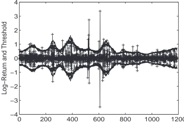
rare events of very high intensity. Many discontinuities of smaller amplitude affect the behavior of assets: on the average we can identify, visually, 5_{− 10 of such abrupt variations per year. Such kind of rapid and} intense variations are usually referred as jumps. In this context we expect that, after a jump has occurred, the market switches in a new status characterized by an high level of volatility. As a consequence jumps are expected to have a predictive power on the future behaviour of assets. Despite this is a very intuitive fact it has not yet proved in the financial literature. A volatility forecasting model requires the definition of a volatility proxy. The idea is that proxies adopted in the literature for forecasting purposes are, in fact, contaminated by the presence of jumps in finite sample. In this context the forecasting power of jumps on future volatility cannot be revealed.

In order to highlight such a feature it is needed a precise estimate of the jump component. In this spirit we propose in Chapter 3 a powerful jump separation technique and we test its performances on eight markets of electricity. The separation technique we adopt is taken from very recents results of the financial literature and only requires the introduction of a threshold. In Chapter 4 we construct precise volatility estimators using the threshold separation technique. This approach allows for a volatility estimation unaffected by jumps. Moreover in Chapter 5 we show that a jump purified estimate of volatility allow for a better investigation of its memory properties. Finally in Chapter 6 we construct a volatility forecasting model based on the proposed estimators. Being based on an accurate separation of continuous and discontinuous component of volatility, the model reveals the forecasting power of jumps on future volatility. Moreover we find that the forecasting power of jumps extend to at least one month. A dazzling example of the turbulence triggered by discontinuous variations is the recent crisis of markets. In September 2008 a global big crash has occurred in most part of stock exchanges. Since ever markets show an high level of volatility, characterized by large returns of both negative and postivie intensity. In this sense our results are very topical and constitute a basis for further investigations.

(4)

Economic Equilibrium: The Role of

Thermodynamic Efficiency

This chapter is inspired from the paper of Roma and Pirino (2008).

1.1 Overview and Criticism of General Equilibrium Theory

Microeconomics is a discipline devoted to the investigation of individual decision making. Production of goods and consumption is analyzed in the microeconomic theory from an abstract point of view. This section briefly describes the fundamental principles of the theory which will be frequently used throughout all the chapter.

The scenario is composed of two parts: the producer who releases goods in the market and tries to maximize his profits and the consumer who buys goods and maximizes the utility derived from the goods themselves.

At the equilibrium point profits and utilities are maximized simultaneously. Usually the maximum is reached within some constraints which describe maximum expense sustainable by the consumer, producer’s maximum production capability and so on.

The general equilibrium depends on the production technology used by the producer. Economic pro-duction is usually modelled ignoring the underlying thermodynamic mechanism which brings consumption goods to the market, despite it frequently involves physical processes.

Our goal is to show, focusing on a particular production process, how economic equilibrium is changed when thermodynamic laws are taken into account. We are especially interested on the consequences of thermodynamic irreversibility.

We will show that if the production process is irreversible then the producer is forced to a more parsimonious use of energy, while energy itself is found to play no particular role if the process is reversible.

The theoretical approach described in what follow is taken from Colell et al. (1995).

(8)

CHAPTER 1. ECONOMIC EQUILIBRIUM: THE ROLE OF THERMODYNAMIC EFFICIENCY 2

1.1.1 Preference and Choice

Individual choice behaviour is usually modelled introducing a set of alternatives X. It is an abstract set because alternatives could be everything: take an holiday in Spain, France, Germany etc. It is assumed that the alternative presented by X are mutually exclusive.

The preferences on X are described by a binary relation between any two elements of X. We indicate this relation by _{º and we say that ”x is at least as good as y ” for every x and y in ∈ X such that x º y.} Other important relations are the strict preference relation x_{≻ y defined by: x º y but not y º x,} and the indifference relation defined by: x_{∼ y ⇔ x º y and y º x.}

We assume that the preference relation_{º is rational i.e. it respects the following properties:} • ∀x, y ∈ X we have that x º y or y º x or both.

• ∀x, y, z ∈ X if x º y and y º z then x º z.

It can be shown that ifº is rational then ≻ is irreflexive (x ≻ x never holds) and transitive (if x ≻ y and y _{≻ z then x ≻ z ) while ∼ is reflexive (∀x, x ∼ x) and symmetric (x ∼ y ⇒ y ∼ x).}

In order to represent preferences as real numbers microeconomic theory refers to the concept of utility functions:

Definition 1.1.1 A function u : X_{→ R is a utility function representing preference relation º if ∀x, y ∈ X} it happens that:

x_{º y ⇒ u (x) ≥ u (y) .} (1.1)

Relation (1.1) establishes, in some sense, that the preference is kept unchanged by the utility function in the real line. If u (x) is a utility function then any strictly increasing function f : R→ R define a new utility function v (x), which describes the same preferences as u (x), by imposing v (x)≡ f (u (x)).

1.1.2 The Consumer’s Problem

In our market model the consumer faces the problem of how to choose optimal consumption level for all commodities (and services) that are available for purchase. For the sake of simplicity suppose we have a finite number L of commodities. The consumer must choose for each i = 1, ..., L the optimal level of consumption xi of the i-th commodity. In fact his choice defines a commodity vector (or commodity bundle): x =      x1 .. . xL      (1.2)

which, generally, lies in RL_{. However the set of feasible values for the commodity vector (1.2) is, in fact,} restricted to a smaller set than RL_{. This will become clear when budget constraints will be introduced. As a} first constraint we require that all consumptions level are non-negative, i.e. the consumer is characterized to have only inflows of commodities: debits or outflows are not taken into account. We highlight that

(9)

the entries of vector (1.2) may represent the same commodity at different time: bread today and bread tomorrow are different commodities.

We assume that the price in dollar of all commodities is known. Further it is assumed that the con-sumer’s demand for any commodity is negligible and thus prices are established beyond his influence 1_. The commodity prices are listed in the price vector :

p =      p1 .. . pL     ∈ R L_. _(1.3)

Note that in this context price could be negative. A negative price could be paid by the consumer for the consumption of bad goods like pollution. However in our model prices are restricted to the positive semi-space RL+_.

The consumer is supposed to have a finite amount of dollar to be spent on the market. We call this quantity the total wealth w.

As a consequence a commodity bundle x∈ RL+ _{is affordable only if its total cost is less or equal than} the consumer’s total wealth, in formula:

p· x = p1x1+ ... + pLxL≤ w. (1.4)

As a natural consequence, given a price vector p and the total wealth w, we define the competitive budget set as: Bp,w=©x∈ RL+|p · x ≤ wª.

We have now the correct theoretical tools to formalize the consumer’s decision making problem. As anticipated consumer’s preference are represented by a utility function u (x). Therefore consumer will choose, among all affordable commodity bundles, the one that maximizes his utility. In formula:

Consumer’s Problem: max

x∈Bp,w

u (x) . (1.5)

1.1.3 The Producer’s Problem

On the other side of the economy there is an agent, the producer, who is capable to produce goods to be consumed. This could be, for example, a legally recognized firms. The typical approach consists in modelling the producer as a ”black box” able to transform inputs in outputs. This approach completely ignores internal management issues and the underlying process required for the transformation of basic goods in elaborated ones. We do not know how inputs become outputs, but only that a given amount of input is transformed in a known amount of output 2_{. The production possibilities are described by a} production vector :

1_{This is known as the price-taking assumption.}

2_{This is one of the key point we will criticize. Our approach provide a detailed thermodynamic description of the production}

(10)

CHAPTER 1. ECONOMIC EQUILIBRIUM: THE ROLE OF THERMODYNAMIC EFFICIENCY 4 y =      y1 .. . yL     ∈ R L _(1.6)

where yi indicates the amount of the i-th commodity used or produced. We use the convention that negative entries of (1.6) describe input goods while positive quantities indicates output commodities. For example y = (−2, 1, 0) indicates that 2 units of good number one are used to produce 1 unit of the good number two, while commodity three is not used nor produced.

Given a specified production technology not all y _{∈ R}L _{are feasible production vectors. In order to} understand this limitation one should think to the finite capacity of each production plant and to the minimum inputs required to carry out production. We postulate that there exist a set Y_{⊂ R}L _{such that} if y_{∈ Y then y is possible while any y /}_{∈ Y is not.}

We focus on production model with one single output. In this case it is convenient to introduce the production function i.e. the maximum level of output produced for a given set of inputs. If_−y1, ...,−yL−1, with yi≥ 0, indicate the input quantities and q = yL≥ 0 is the correspondent output then the production function f is such that q ≤ f (y1, ..., yL−1). The maximum production is obtained when q = f (y1, ..., yL−1). It is clear that f should describe, in some way, the technology used to carry out production. Suppose that all production inputs are multiplied by a constant factor λ. Three cases may arise:

• f (λ y1, ..., λ yL−1) = λ f (y1, ..., yL−1), which is referred as constant return to scale. • f (λ y1, ..., λ yL−1) < λ f (y1, ..., yL−1), which is referred as decreasing return to scale. • f (λ y1, ..., λ yL−1) > λ f (y1, ..., yL−1), which is referred as increasing return to scale.

Once the production technology is specified by the production function the producer tries to maximize its profits:

Consumer’s Problem: max

y∈Y p1y1+ p2y2+ ... + pLyL, (1.7) where p1, ..., pL are the price vector components introduced in (1.3). At the equilibrium point we suppose that supply equals demand, this assertion is known as market clearing condition. A set of price p that realizes perfect balance between demand and supply is called a market clearing price. In formula the clearing condition is written as:

∀i = 1, ..., L if yi≥ 0 ⇒ xi= yi. (1.8)

The condition yi ≥ 0 implies that a quantity of the good i is produced and released on the market, therefore equality xi= yi resets disparities between demand and supply.

(11)

1.1.4 Two Commodities Models

Suppose we have two commodity (L = 2) which are the same physical good produced at two different times, for example a mineral today and the same mineral tomorrow. On the consumer’s side we have:

max x1p1+x2p2≤w

u (x1, x2) . (1.9)

First order conditions imply that:

∂u ∂x1 − λ p1 = 0, (1.10) ∂u ∂x2 − λ p2 = 0, (1.11)

where λ is a Lagrange multiplier: λ6= 0 when x1p1+ x2p2 = w while λ = 0 when x1p1+ x2p2 < w. Suppose that the consumer spends all his wealth w on the market, thus λ6= 0. From equations (1.10)-(1.11) we find that: p2= p1 Ã ∂u ∂x2 ∂u ∂x1 ! . (1.12)

Equation (1.12) states that, at equilibrium, the price of the good 2 is given multiplying the price of good 1 by the factor:

B_≡ ∂u ∂x2 ∂u ∂x1 . (1.13)

In our case, commodities one and two are the same physical good at different times, thus we can interpret B as a discount factor. On the producer’s side of the economy we have:

max

y∈Y p1 (y1+ B y2) , (1.14)

having used relations (1.12)-(1.13). Solution of problem (1.14) is independent of p1which appears only as a multiplying factor. This is a well-known result of neoclassical economic theory usually referred as neoclassical paradigm.

Price is usually called numeraire and it expresses the chosen mean of exchange in our economy. Neo-classical paradigm states that the economic equilibrium is indifferent to the choice of the numeraire. We can choose to price commodity in apples, potatoes or a single currency without changing the equilibrium established between consumers and producers.

1.1.5 Isoquants and Substitutions

Suppose that a production function exists. For the sake of simplicity we further require that the production is based on only two inputs_−y1and−y2. They could be capital and labour or energy and raw material to be refined etc. An isoquant at level K is defined as the lieu of points (y1, y2) such that f (y1, y2) = K. We wonder whether it is possible to preserve the same level of production K allowing one between y1 and y2 to go to zero. This problem arises in concrete situations when one of the two inputs is scarce or even null.

(12)

CHAPTER 1. ECONOMIC EQUILIBRIUM: THE ROLE OF THERMODYNAMIC EFFICIENCY 6 In other words: how much quantity of y1is necessary to compensate a loss in y2(and vice versa) keeping production at the same level? We will say that y1 and y2are perfect substitute when every loss in one of the two variables can be compensate with a proper increase in the other. This idea could be extended to an arbitrary high number of input variables. As an example a linear technology like f (y1, y2) = a y1+ b y2 allows for perfect substitutability of inputs. In literature, most specifications of production functions allow for a complete or a partial substitution between variables.

1.1.6 Some Criticism of Neoclassical Theory

In this chapter we provide an overview of the current research on substitutability among production inputs and production function modelling. Our goal is to show how substitutability among inputs is limited when a thermodynamic approach is taken. We will focus on the production of a refined mineral which is obtained using as inputs energy and raw material. As the thermodynamic intuition suggests, the substitution between these two inputs is limited by physical constraints. The production function derived from a full thermodynamic model incorporates directly these constraints providing a more realistic description of the production process. We further study the consequences of irreversibility on economic equilibrium. We will show that neoclassical equilibrium is drastically changed when irreversibility is taken into account in the production technology. We also find that, when a finite time thermodynamic model is adopted, energy plays an important economic role. Moreover the decision making strategy is completely changed when the production process is reversible i.e. it is carried out in an infinite time. We will show that reversible technology reproduces the same results one would obtain in the neoclassical theory with a linear technology. In this sense ignoring irreversibility is equivalent to allow for unrealistic perfect substitutability among inputs.

1.2 Introduction

The centrality of the role of energy as an input in the production process of economically valuable goods is difficult to dispute. Yet in economics a consensus on how this should be modeled has not emerged. The resource degradation connected with its use suggests energy warrants a specific treatment as a factor of production. Intensive energy use creates environmental damage through the release of residual heath. As discussed in the seminal contribution of Georgescu-Roegen (1971), the second law of thermodynam-ics, which governs energy utilization and degradation, is a key source of negative externalities. In the production literature a limited amount of attention has been dedicated to the concept of waste as an unavoidable joint product of any production process (Ayres and Kneese, 1969; Ethridge, 1973; Kum-mel, 1989). Traditional economic analysis of production generally avoids thermodynamic considerations. Typical production models require substitutability between any inputs none of which, including energy, has a special role. On these premises the economics literature dealing with the use of energy has largely focused on the possibilities for substituting it as a factor of production in the presence of energy price shocks or energy shortages. 3 _{Factors of production (as well as consumption goods) are interchangeable}

3_{Abel (1983) proposes a model for the substitution between energy and capital in a generic production function when}

(13)

if they provide the same functionality. The complete substitutability among natural resources (including energy), labor and capital leads however to paradoxical consequences. Daly (1997) observes that, if labor and natural resources are substitutes and not complements then it would be possible to make a cake with ”[...]only the cook and his kitchen. We do not need flour, eggs, sugar, etc., nor electricity or natural gas, nor even firewood. If we want a bigger cake, the cook simply stirs faster in a bigger bowl and cooks the empty bowl in a bigger oven that somehow heats itself[...]”. A dazzling example of this paradox can be found in the standard representation of funds and flows in the Cobb-Douglas production function model, that is:

Q = Kα1_Lα2_Rα3_, _(1.15)

where Q is the output of the process per unit of time, K represents the stock of capital, L the labor supply and R the flow of natural resources. From expression (1.15) it is evident that we can obtain a fixed amount of output Q0even if R→ 0, it is sufficient to choose an amount of K such that:

K = µ Q0 Lα2Rα3 ¶1 α1 → +∞. (1.16)

Although it is well understood that the Cobb-Douglas production function (as well as its extension) is only an abstract concept and not an actual description of a production process, this very concept has a pervasive influence on economic modeling. Substitutability plays a critical role in the Neoclassical general equilibrium construction. It underlies the view that there are no real limits in the economic growth as, in the extreme, ”the world can, in effect, get along without natural resources” Solow (1974). Incidentally, Neoclassical general equilibrium also implies the substitutability of every good as a numeraire and means of payment. Still this is a useful framework which yields insight on the value and optimal exploitation over time of non-renewable resources (Hotelling, 1931).

It may be sensibly argued, as Ayres and Miller (1980) put it, that there are definite and well-known limits on physical performance in almost every field which derive from the unique role of some specific factor of production. Energy is a case in point. See Cleveland and Ruth (1997) for a survey of the literature

four level of inputs: capital, labor, energy and materials. The effect of unpredictable energy price variations is analysed in a real business cycle model by Kim and Loungani (1992), explicitly incorporating energy as an input in a CES production function. A vast number of papers are dedicated to the empirical analysis of capital-energy substitution, which is of ”great importance in predicting economic disruptions arising from energy shortages” (Field and Grebenstein, 1980). The papers of Berndt and Wood (1975) and Fuss (1977) highlight a negative value for the capital-energy substitution elasticity, indicating that they are not substitutes, while Griffin and Gregory (1976) and Pindyck (1979) find a positive value. The discrepancy is fully explained in Field and Grebenstein (1980) who find that the difference between the two results lies in the way the capital input is handled. A paper by Magnus (1979) remarks that energy inputs interact differently with labor (in a substitutable way) and capital (in a complementary way) and this justifies the introduction of energy as an independent input in the production function. The work of Atkenson and Kehoe (1980) sheds light on the fact that, with respect to the energy prices, energy use is inelastic when dealing with time-series data and elastic with cross-sectional data. They develop a putty-putty model and a putty-clay model which reproduce these differences in elasticities. Finally, the difference between cross-sectional data and time series data in capital-energy substitution elasticity is resolved by Thompson and Taylor (1995) using Hiroshima elasticities. Arrow et al. (1961) provide an exhaustive analysis of capital-labor substitutability, concluding that the substitution elasticity between capital and labor in manufacturing may typically be less than one.

(14)

CHAPTER 1. ECONOMIC EQUILIBRIUM: THE ROLE OF THERMODYNAMIC EFFICIENCY 8 covering this alternative point of view. However, such analyses are often of a qualitative nature. The case for (the lack of) substitutability can be often argued either way due to the vagueness of the approach.

As a contribution to this debate we provide a robust theoretical foundation for the lack of substi-tutability of the energy input in the extraction and refinement of a commodity. Specifically, we propose an analytic model for a mining operator who refines a mineral from its natural concentration to a strike con-centration which defines the product. Consistently with actual physical constraints the production process is modelled analytically, following the thermodynamic theory of an irreversible separation process.4.

All real world transformations involving energy are in fact irreversible. A thermodynamic transforma-tion or cycle is said to be reversible if it is carried out by varying a state variable with infinitesimal changes that allow the system to be at rest throughout the entire process (Fermi, 1956). Such a transformation is impossible because it would require an infinite amount of time. All production processes are therefore irreversible in nature, because they have to be carried out in a finite time-period to bring production to the market. They involve then a strictly positive increase in entropy ∆ S > 0. An increase in entropy means a reduction in ”useful” energy, that is the part of energy that can be converted into work by an engine. Thus an entropy increase can be interpreted as waste or resource degradation. If the production function does not accommodate the real thermodynamic process which leads to the final consumption good, the impact of the producer’s choices on resource depletion and the waste released on the environment will not be evident.

The derivation of our production model is driven by the pursuit of the maximum efficiency in the use of available energy so that the least possible amount of it is required. Despite the attempt to minimize its use as an input a positive energy amount is always necessary to extract the natural resource. For the specific case, this lower limit provides an answer to all issues raised by the recent and past literature about substitutability between production process inputs. Although limited substitution of energy is possible, total substitution is impossible because there is a physical energy threshold, for a given quantity of raw material input, below which no production exists. This emphasises the importance of a physics-based approach to production modelling as a correct methodological way of resolving the substitutability issue. A standard Cobb-Douglas model would lead to results in contradiction with the laws of nature (Islam, 1985)5_.

Except for a few papers microeconomic analysis completely avoids a detailed consideration of the physical constraints which are the essence of every production process.6_{. Krysiak and Krysiak (2003) study} the impact of the first law of thermodynamics on the standard general equilibrium model of production and consumption. They show that general equilibrium theory is consistent with the mass and energy conservation laws. Krysiak (2006) analyzes the consequences of the second law of thermodynamics on

4_{A number of papers deal with the decisions concerning the exploitation of physical resources and the}

extrac-tion/production of commodities (Brennan and Schwartz, 1985; Coratzar et al., 1998; Hartwick, 1978; Stiglitz, 1976) but none describes the thermodynamics of extraction.

5_{A list of economic key-objections and economic advantages of the Cobb-Douglas function can be found in Murthy (2002).} 6_{Sav (1984) uses a micro-engineering production function derived from physical laws to model the exploitation of solar}

energy for domestic water heaters. Substitution elasticities between nonrenewable fuel inputs (oil or natural gas) and capital-intensive solar-produced heat is investigated. In this context Sav (1984) finds that a governmental taxation policy for solar energy incentives could paradoxically result in an increase in consumption of nonrenewable energy resources.

(15)

economic equilibrium in a general framework, arguing that if irreversibility is taken into account a non-zero level of inputs and a non zero-level of emissions are necessary to sustain a positive level of consumption7_. A production function derived from finite time thermodynamic constraints can be found in Roma (200), Roma (2006), who proposes a general equilibrium model for the production of a basic good (hot water) based on a fully consistent thermodynamic description of the process. The production process we analyze here from a physical point of view differs from the hot water production process in Roma (2006) in that the final product obtained will be of homogeneous quality and unused energy can be stored.

An important precedent for our commodity extraction problem is Ruth (1995). This paper contains explicitly thermodynamic constraints on production in the form of lower bounds on the inputs to be fed into a Cobb-Douglas production function. The lower energy bound is calculated for a reversible separation process. As mentioned above, this approach does not reflect the reality of production, which involves only irreversible processes. The degradation of energy is far higher in irreversible processes than in the reversible ones and irreversible processes make a greater contribution to entropic increase, as stated by the second law of thermodynamics.

We then turn to the analysis of the rational use of energy from an economics point of view. Berry et al. (1978) highlight the difference between the concepts of thermodynamic optimality of the use of energy in production and overall economic (cost) efficiency. The economic notion of Pareto optimality for resource allocation (where no individual can be better off without making al least one other worse off) will not in general amount to the optimal use of available energy from a thermodynamic point of view. If energy is in aggregate scarce and becomes a limiting factor because of its lack of substitutability (as argued by Ayres and Miller, 1980) the two criteria may indeed coincide.

We are able to carry further the analysis in Berry et al. (1978). They do not model the thermodynamic properties of the technology and assume that substitution of energy by other inputs along a production isoquant amounts to an increase in thermodynamic efficiency. As thermodynamic efficiency cannot be increased beyond the reversible limit full substitutability of energy is prevented, i.e. it is impossible to move beyond a certain point on the isoquant in the energy dimension.

We can analytically derive instead the production isoquants under the assumption of maximum finite time thermodynamic efficiency (a possibility dismissed by Berry et al. (1978) as optimistic, see p.133). Hence in our world engineers make sure that production is achieved in any case with maximum thermo-dynamic efficiency. This is still compatible with some (quite limited) amount of substitutability between anergy and raw material.

We analyse the problem of the optimal scale of production and the consequent exploitation of natural resources, including energy, under the finite time thermodynamic foundation adopted. Even if the the most efficient thermodynamic technology is used higher production in the same amount of time implies greater deviation from reversible efficiency and higher energy waste. Hence it is the scale of production which determines in the end thermodynamic efficiency.

7_{On the debate about the impact of the entropy law on economic equilibrium see also Young (1991) and Daly (1992)}

which lead to two completely opposite conclusions. Many authors have investigated Nicholas Georgescu-Roegen’s paradigm of ecological economics, again obtaining conflicting conclusions, such as those reported by Khalil (1990), subsequently criticized by Lozada (1991) and finally re-stated by Khalil (1991).

(16)

CHAPTER 1. ECONOMIC EQUILIBRIUM: THE ROLE OF THERMODYNAMIC EFFICIENCY 10 We incorporate the production model in a simple general equilibrium framework in which we analyze production decisions. We derive the equilibrium in a simple economy in which our good is produced and consumed and address in this context the role of energy efficiency in optimal economic decisions. In a neoclassical equilibrium the optimal allocation of available resources will follow from the non-satiated demand for final goods and the efficiency in the use of available energy will not drive on its own economic decisions. Under a Neoclassical model the amount of thermodynamic waste will be irrelevant and nat-ural resources will be fully exploited. On the other hand, the negative externalities associated with the degradation of energy, if taken into account, would lead to a thermodynamic efficiency criterion in the use of this scarce resource. However, thermodynamic efficiency would have to be imposed on the decision makers (by way, for example, of a ”green tax”). We find, similarly to Roma (2006), that a competitive economic equilibrium will be twisted towards higher thermodynamic efficiency if energy is forced to be the numeraire and means of payment. This creates a market in which the energy price of production is established. If energy is the only scarce factor the producer will compare the energy cost of production with the energy value of the firm’s sales determined by supply and demand. The lack of substitutability between input factors and the decreasing return to scale feature of irreversible technology imply that part of the energy available in the economy will not be used in production. This will in turn decrease energy degradation and thermodynamic waste. The neoclassical solution, where a change in numeraire and means of payment would not alter the neoclassical equilibrium, is finally obtained if the production process is carried out over an infinite time, i.e. if it is reversible. Reversibility is equivalent to constant returns to scale technology.

This chapter is organized as follows: Section 1.3 is dedicated to a description of the physical process underlying the production of the commodity. Here the thermodynamic production function is derived together with the marginal and average costs of production. Isoquants of the computed production function are compared with those derived from a Cobb-Douglas type production function, in order to highlight the differences between the two approaches. Section 1.3.2 briefly describes the idea by Ruth (1995) of a thermodynamic limit on production inputs. The problem of a producer who uses a thermodynamic production function and faces scarcity of energy is presented in Section 1.5. After introducing the concept of Energy Return on Energy Investment (EROEI), energy will be used as the numeraire and means of exchange in our economy. It is shown that, when energy is scarce, and it cannot be substituted, the producer’s decision varies drastically if the accounting is made in terms of energy or in terms of another numeraire (such as the product itself). The consumer’s problem is also described in this section. Section 1.7 shows that arbitrage arguments can be stated in a perfectly reversible context to compute the price of the commodity in terms of energy, while the same arguments weaken if irreversibility arises. The producer’s choices under a reversible technology are discussed in Section 1.8. Finally, in Section 1.9, we present our conclusions.

1.3 The Physical Model

Thermodynamic energetic limits to industrial processes have been analyzed by a vast number of authors. The survey of Sieniutycz (2003) provides an exhaustive analysis of the most commonly used methods

(17)

for computing thermodynamic energy limits to industrial production, such as separation processes, heat pumps, chemical and electrochemical systems, maximum power in thermal engines, etc. Energy limits in industrial processes are investigated from a classical thermodynamic approach by Forland et al. (1988), Kim and Loungani (1985), and Denbigh (1956). Engineers typically face the problem of how to set-up a production plant capable of achieving non-zero production in a finite time and with finite industrial facilities. In most cases this kind of problem is solved using one of two alternative approaches: finite time thermodynamic (Andersen et al., 1977; Berry et al., 2000) or entropy generation minimization (Bejan, 1996; Nummedal et al., 2005; Salamon et al., 1980), which are usually referred as FTT and EGM, respectively. The idea underlying these approaches is that energy is a scarce resource and its use must be optimized.

The physical model adopted for the construction of our production function is developed by Tsirlin and Titova (2004). They compute (via EGM) the minimum energy required to achieve the separation of an ideal mixture of components with a specified output.

Figure 1.1: The scheme used by Tsirlin and Titova (2004) to model the separation of a finite subsystem from an infinite reservoir. The thermodynamic state of the reservoir is identified by the temperature T , the pressure P and the composition vector C0. The pumps g0 and g1 are the mass-transfer coefficients from the reservoir to the working medium and from the working medium to the reservoir respectively. The working medium has a chemical potential µP

0 at the contact point with the reservoir and a chemical potential µP

1 at the contact point with the subsystem.

Figure 1.1 illustrates the scheme used to model the process. A subsystem to be separated out is in contact with an infinite reservoir characterised by a temperature T and a pressure P which do not vary during the transformation. This may be interpreted as a stylized production plant in which a valuable substance with pre-specified purity must be refined and extracted from the original mixture of substances which are found in a natural reservoir. The extracted substance is accumulated in the subsystem.

The mining operator faces an initial mixture of useful mineral and waste rock. We suppose that the mineral is initially a minority presence with respect to the waste rock and the mining operator tries to purify the mixture and extract highly concentrated mineral8_.

8_{A number of papers deal with the decisions concerning the exploitation of physical resources and the}

(18)

CHAPTER 1. ECONOMIC EQUILIBRIUM: THE ROLE OF THERMODYNAMIC EFFICIENCY 12 At time t = 0 the composition vector of the reservoir, which describes the (percentage) concentrations of the different mixture components, is (C01, ..., C0n). The subsystem is initially at equilibrium with the reservoir and is therefore characterised by the same thermodynamic variables T , P and by the same com-position vector (C01, ..., C0n) as the reservoir. We indicate with N0 the number of moles in the subsystem at t = 0.

Separation processes and chemical reactions are usually described by means of chemical potentials. We recall that the chemical potential of a substance in a system represents the variation of the system’s internal energy when a unit of the substance is added, keeping system’s volume and entropy constant.

Each component of the mixture has a chemical potential µ0i(T, P ) in the reservoir which depends on its concentration C0i and is given by:

µ0i(T, P ) = µ0(T, P ) + R T log C0i, (1.17) where R is the universal gas constant and µ0(T, P ) represents the reservoir chemical potential which does not vary during the transformation. We can interpret µ0(T, P ) as the ground level from which all other chemical potentials are measured. As it is only a scale variable we could impose µ0(T, P ) ≡ 0. However we choose to leave µ0(T, P ) unspecified for the sake of generality.

The subsystem and the reservoir are in contact with a third medium, a working medium, which has the chemical potentials µP

0 and µP1 at the contact points with the reservoir and the subsystem respectively. This is a short-hand notation to indicate that the i-th component has a chemical potential µP

0i at the contact point with the reservoir and µP

1i at the contact point with the subsystem. A working medium is simply defined as a system whose chemical potentials are under control. When in contact with the reservoir and the subsystem, the working medium generates chemical potential drops between the contact points. Particles tend to diffuse from regions of high chemical potential to regions of low chemical potential, allowing for the mass transfer.

Examples of mixture separation with the formalism of chemical potentials can be found in Wijmans and Baker (1995) and Vallieres et al. (2003). As observed by Wijmans and Baker (1995) a chemical potential variation dµiof the i-th mixture component across a membrane of thickness dx produces a mass flux given by:

Ji=−Li dµi

dx, (1.18)

where Liis a coefficient of proportionality. All driving forces such as gradients in pressure, temperature, concentration and electromotive forces can be reduced to chemical potential gradients and, therefore, they generate mass fluxes which can be expressed in the form (1.18).

Through this mechanism the working medium creates a mass flux g0i of the substance i between the reservoir and the working medium, and a mass flux g1i of the substance i between the working medium and the subsystem. All these fluxes have the dimension of mole per time: [g] = [mol] [time]−1. Following the approach of Onsager (1930), Onsager (1931) and Miller (1994), it is assumed that the system is close to equilibrium. More precisely, as described in Miller (1994), ”one divides the system

(19)

into small subsystems and assumes that each subsystem is in local equilibrium, i.e., it can be treated as an individual thermodynamic system characterized by the small number of equilibrium variables.”. This common assumption leads to linear irreversible thermodynamics, in which the relation between chemical drops and mass transfer coefficient is linear (Onsager’s Kinetics).

At the final instant t = τ the subsystem has a new specified composition vector (Cτ 1, ..., Cτ n) and contains a number of moles Nτ. Following the reasoning in Tsirlin and Titova (2004), the separation work in an isothermic process (i.e. with temperature kept constant) for an adiabatically insulated system (i.e. heat exchanges are not allowed) is given by the Gouy-Stodola formula:

E = E0+ T ∆S, (1.19)

where E0 is the reversible work and ∆S the entropy increment. The reversible work is computed summing the total internal energy variation of the reservoir to that of the subsystem. The internal energy variation of the reservoir is easily computed observing that a number of moles ∆N = Nτ− N0 leaves the reservoir. The component concentrations in the reservoir do not change during the process, the reservoir being infinitely large. Therefore for each mixture component i we have that a number of moles ∆N C0i leave the reservoir. According to the definition of chemical potential the total internal energy variation of the reservoir ∆URes is given by:

∆URes = n X i=1

(_{−∆ N) C}0iµ0i(T, P ) . (1.20)

Using relation (1.17) and recalling thatPn_i=1C0i= 1 we obtain: ∆URes = " (−∆N) µ0(T, P ) + R T n X i=1 (−∆N) C0i log C0i # . (1.21)

Within the subsystem the initial number of moles of each component is N0i = N0C0i and after the separation process has operated for a period of time τ the final number of moles becomes Nτ i = NτCτ i. At time t = 0 the subsystem is in equilibrium with the reservoir, therefore each mixture component has an initial chemical potential given by (1.17). At the final instant τ , the chemical potential of the i-th component in the subsystem will be µ0(T, P ) + R T log Cτ i.

Therefore the total internal energy variation ∆USub of the subsystem is given by:

∆USub = n X i=1 [Nτ iµτ i− N0iµ0i] = (1.22) n X i=1 [NτCτ i (µ0(T, P ) + R T log Cτ i)− N0C0i (µ0(T, P ) + R T log C0i)] = (1.23) µ0(T, P ) ∆N + R T " Nτ n X i=1 Cτ i log Cτ i− N0 n X i=1 C0i log C0i # , (1.24)

where we have used the conditionsPni=1C0i =Pni=1Cτ i= 1. The sum ∆URes + ∆USub returns the total reversible energy required for the separation process:

E0= ∆URes + ∆USub = NτR T n X i=1

(20)

CHAPTER 1. ECONOMIC EQUILIBRIUM: THE ROLE OF THERMODYNAMIC EFFICIENCY 14 and it is independent of N0. Note that, as expected for a state-function, formula (1.25) only depends from the initial and final states of the system, Cτ i, C0i i.e. it is path-independent9. For this reason a minimum entropy increment ∆S corresponds to the minimum value for E in (1.19). The entropy increment corresponding to the mass transfer coefficients g0i is given by:

∆S = 1 T Z τ 0 n X i=1 £ g0i¡µ0i− µP0i ¢ + g1i ¡µP1i− µ1i¢¤dt = 1 T Z τ 0 n X i=1 [g0i∆µ0i+ g1i∆µ1i] dt, (1.26) where µ1i is the chemical potential of the i− th component in the subsystem. The parameters of the working medium do not change within a cycle, therefore:

i = 1, ..., n. Z τ 0 g0idt = Z τ 0 g1idt. (1.27)

Moreover the mass balances impose that:

i = 1, ..., n.

Z τ 0

g1idt = NτCτ i− N0C0i. (1.28) The problem of minimizing the energy (1.19) is then reduced to the following one:

min g0i,g1i 1 T Z τ 0 n X i=1 [g0i∆µ0i+ g1i∆µ1i] dt, (1.29) sub Z τ 0 gjidt = NτCτ i− N0C0i, j = 0, 1. i = 1, ..., n.

In the case of an Onsager’s kinetics (see discussion above) we have that gij = αij∆µij, and it can be shown that (Tsirlin and Kazakov, 2004; Tsirlin et al., 1998) optimal solutions of problem (1.29), under this additional assumption, are constant mass transfer coefficients. From conditions (1.27)-(1.28) we immediately obtain:

j = 0, 1. i = 1, ..., n. gji= NτCτ i− N0C0i

τ . (1.30)

In order to put formulas in a simpler form we define the total mass variation of the i-th component:

∆ (N Ci)def≡ NτCτ i− N0C0i, (1.31) and we introduce the equivalent mass-transfer coefficient:

¯ αi def ≡ _αα0iα1i 0i+ α1i . (1.32)

Substituting optimal solutions (1.30) in expression (1.26) we obtain the entropy variation. It follows that the minimum energy required to carry out the transformation [N0, (C01, ..., C0n)]→ [Nτ, (Cτ 1, ..., Cτ n)] in a finite time τ is:

(21)

Emin= R T Nτ n X i=1 [Cτ ilog Cτ i− C0ilog C0i] + 1 τ n X i=1 [∆ (N Ci)]2 ¯ αi . (1.33)

In the simplest case the valuable substance may be assumed to be mixed with only one other, so the initial vector of concentrations is (C0, 1− C0). For example, C0 can be the concentration of a mineral in the mineral ore and thus 1− C0 can be interpreted as the waste rock concentration.

Differently from Ruth (1995), who adopts the extreme assumption that the mineral can be completely separated from the waste rock, we generalize the definition of the final product and define it more real-istically as mineral extracted with a given strike concentration k > C0 but still mixed with a residual concentration 1_{− k of waste rock. With n = 2, (C}01, C02) = (C0, 1− C0) and (Cτ 1, Cτ 2) = (k, 1− k). Therefore (1.33) takes the form:

E = R T Nτ [k log k + (1− k) log (1 − k) − C0 log C0− (1 − C0) log (1− C0)] + (1.34) + 1 τ α h (Nτk− N0C0)2+ (Nτ (1− k) − N0(1− C0))2 i ,

where we have imposed, for simplicity, ¯α1 = ¯α2 ≡ α. The second term on the right hand side of expression (1.34) denotes the irreversible use of energy. It involves the square of the difference Nτk−N0C0 between the refined moles extracted and the moles of pure material in the subsystem, and the corresponding difference Nτ (1− k) − N0(1− C0) for the waste material.

As a final remark note that the optimal coefficients g0i, g1i define the speed at which the extraction plant must be operated in order to waste the minimum possible amount of useful energy. This type of efficiency is clearly desirable for any production plant. However it clearly limits the speed of production, although it is conceivable to operate the plant faster if energy were not a scarce resource. On the other hand the scale of production, which is given by Nτ , is a free choice. The energy required for the separation is a monotonically increasing function of Nτ. For a given level of output Nτthe production technique defined by (1.34) leaves a choice between extracting the actual amount at the desired level of concentration or, where possible, “averaging up” the concentration of an amount N0 of the original mixture already contained in the subsystem. This is the source of the limited substitutability between N0 and E. As a special case of (1.33) the minimum energy required to separate completely the two components contained in N0 moles of a binary mixture is (Tsirlin and Titova, 2004):

Ebinm =−R T N0[C0 ln C0+ (1− C0) ln (1− C0)] +N 2 0 τ Ã C02 ¯ α1 +(1− C0) 2 ¯ α2 ! , (1.35)

where ¯α1and ¯α2 are the parameters defined in (1.32).

1.3.1 The reversible limit

The reversible increment in the internal energy of the system which is required for production can be computed taking the limit for τ → +∞ of equation (1.34):

(22)

CHAPTER 1. ECONOMIC EQUILIBRIUM: THE ROLE OF THERMODYNAMIC EFFICIENCY 16 where NR are the number of moles produced reversibly. Equation (1.36) says that the transformation [C0, 1− C0]→ [k, 1 − k] requires a positive amount of energy for the pairs (C0, k) such that:

ξ0≡ k log k + (1 − k) log (1 − k) − C0log C0− (1 − C0) log (1− C0) > 0. (1.37) We assume that our mineral is initially available at a minority concentration, namely C0 < 1₂. We try to purify the substance in order to obtain a strike concentration k such that 1_{− C}0 < k, which is greater than the initial concentration of the waste rock. In this framework ξ0> 0 and the number of moles produced when τ _{→ +∞ is:}

NR= E

R T ξ0

. (1.38)

1.3.2 Ruth (1995) Model of Mining Technology

Ruth (1995) presents the problem of the mining operator as the maximisation of a value function essentially defined as the time-integral of production growth minus the growth in energy expenditure for production. Hence his model assumes that the energy input is the only cost of production. To model production, Ruth (1995) uses a Cobb-Douglas type function given by:

Yt= µ_J t− Jt∗ JA− J_A∗ ¶γ1 µ_E t− Et∗ EA− E_A∗ ¶γ2 , (1.39)

where Jt is the raw material input, Et is the energy input and the starred quantities Jt∗ and Et∗ are the minimum material input and minimum energy input required for the production of Yt, respectively. With JA and EA (JA∗ and EA∗), Ruth (1995) indicates the same quantities in a base year.

The Cobb-Douglas production function (1.39) tries to capture the limits to the substitution between energy and raw material that are necessary to produce the quantity of the final good Yt. The lower limit E∗

t is derived as the reversible limit of (1.35) for τ → +∞ (and time varying concentration C0). Still, Et∗ and J∗

t may be partially substituted.

Our approach will be completely different: we will derive the production function Yt from finite ther-modynamic considerations alone. In this approach the limits to the substitution between energy and raw material are represented by an analytical thermodynamic constraint. This production function has very different properties from a Cobb-Douglas function.

1.4 The Production Model

Equation (1.34) implicitly defines a production function Nτ(N0, E), where the inputs are energy, E, and raw material, N0, and where production time, τ , also determines the amount of final product that can be obtained. We can re-arrange expression (1.34) as:

Nτ2 1 τ α h k2+ (1− k)2i+ Nτ · R T ξ0− 2N0ψ0 τ α ¸ +N 2 0 τ α h C02+ (1− C0)2 i − E = 0, (1.40)

where the constants ξ0 ≡ k log k + (1 − k) log (1 − k) − C0 log C0− (1 − C0) log (1− C0) and ψ0 ≡ k C0+ (1− k) (1 − C0) depend only on the initial and final concentrations. The solutions of (1.40) are:

(23)

Nτ±= −R T ξ0+ 2 QτN0ψ0± q (R T ξ0)2− 4 Q2τ(k− C0)2 N02− 4 R T QτN0ψ0ξ0+ 4 GkQ E 2 QτGk , (1.41) where we have introduced the notation Qτ = _{τ α}1 and Gx= x2+ (1− x)2. A solution to the problem exists if, and only if, the quantity under the square root of equation (1.41) is greater than or equal to zero:

δ = (R T ξ0)2− 4 Q2τ(k− C0)2 N02− 4 R T QτN0ψ0ξ0+ 4 GkQ E ≥ 0. (1.42) This condition implies that there is a limited substitutability between process inputs and defines a lower bound on the energy input:

E_≥ 1 4 QτGk h N024 Q2τ (k− C0)2+ N0(4 R T ξ0ψ0Qτ)− (R T ξ0)2 i . (1.43)

Inspecting equation (1.43), we can see that if k _{6= C}0 and N0 > 0, a lower bound on energy always exists for a high enough positive value of N0. In our model of production k > C0, because we want to improve the quality of the valuable substance, and N0> 0 because we assume that our basin is not empty at the initial time10_{. This means that we start production only if the energy is over the threshold given by} equation (1.43). As pointed out by Islam (1985), such restrictions on production inputs drastically modify the isoquants with respect to those of a Cobb-Douglas function.

Only the solution of (1.41), which increases in the energy input, has a physical sense. We then define our production function as:

Nτ(E, N0)≡ −R T ξ0+ 2 QτN0ψ0+ q (R T ξ0)2− 4 Q2τ(k− C0)2 N02− 4 R T QτN0ψ0ξ0+ 4 GkQ E 2 QτGk . (1.44) Expression (1.44) explicitly gives the number of moles of the highly refined mixture (k, 1− k) we obtain starting from N0moles of raw material and spending energy E for production in a finite time τ .

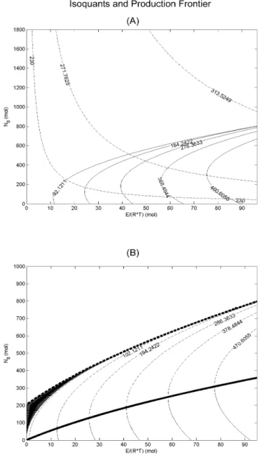
Figure 1.2 shows the isoquants of Nτ(E, N0) for a chosen specification of the model parameters (re-ported in Table 1.1). The chosen values have no particular significance, they have been chosen only for a graphical representation.

The isoquants of (1.44) display an ”economically inefficient” portion, where the same level of production is obtained with more N0 than necessary. We can disregard this portion.

Isoquants derived from a Cobb-Douglas type production function are also reported as thin dotted lines. The plotted Cobb-Douglas function has the form NC−D_{(E, N}₀_{) = A}¡ E

R T ¢γ1

Nγ2

0 and A, γ1 and γ2 are chosen to obtain nearly the same levels of Nτ(E, N0) isoquants.

Using NC−D_{(E, N}₀_{) as a production function would generate perfect substitutability between the two} production inputs, that is given a point³N0(1), E(1)/ (R T )

´

which belongs to an isoquant NC−D(N0, E) = K1 it is possible to obtain the same level of production K1, arbitrarily reducing the quantity of energy entering the process and increasing the number of moles N0of raw material.

10_{As we will show later, energy-efficient production requires a strictly positive value of N}

0 which is proportional to the

(24)

CHAPTER 1. ECONOMIC EQUILIBRIUM: THE ROLE OF THERMODYNAMIC EFFICIENCY 18 Parameter Value T 1250 K k 80% C0 30% τ 3600 sec α 10−4_mol2_{/ (J sec)}

Table 1.1: A set of chosen parameters.

This property disappears when the production function is obtained via the real thermodynamics pro-cess. The constraint (1.43) does not allow perfect substitutability between inputs. This gives a more realistic description of the process and recognizes the different nature of energy as a production input.

Expression (1.44) provides a theoretically consistent production function for the extraction of refined mineral from a low grade mixture. It naturally incorporates a lower bound on the energy input in the spirit of Ruth (1995) and, as anticipated, makes the lack of substitutability between inputs completely clear.

However, we find that the lower bound on the quantity of low grade mixture N0is zero. In what follows, we assume that there is an unlimited quantity of the raw material N0 and it is therefore freely available to the producer, while energy is scarce. In this we follow Ayres and Miller (1980), who argue that basic materials will always be available in some concentration in the earth’s crust, but the availability of energy (work) needed to extract them is, in fact, the only limit to economic growth11_.

11_{Georgescu-Roegen (1979) argued that the degradation of quality materials is, in fact, the real limit to the economic}

growth, rather than the scarcity of energy itself. This approach is criticised by Ayres and Miller (1980), who argue that technical progress can overcome the scarcity of physical resources. They point out that a finite quantity of resources must always be embodied in capital and a limit on economic growth and technical efficiency always exists, due to the finite availability of renewable resources. Their point is that all resources, no matter how they are distributed on the earth, can be extracted if enough energy is available. Thus they conclude that energy is, in fact, the only resource that could ultimately limit economic growth.

(25)

Figure 1.2: (A) The dotted lines are isoquants of a Cobb-Douglas type production function NC−D_(N

0, E) = A¡_{R T}E ¢ γ1

Nγ2

0 , with A = 100 and γ1 = γ2 = 0.1. Continuous lines represent iso-quants of the proposed production function Nτ(E, N0), where the model parameters are those reported in Table 1.1. (B) The plot shows the efficient portion of the production function Nτ(E, N0) isoquants as black continuous lines. The parameters chosen are those reported in Table 1.1. The thin dotted lines are the economically inefficient isoquants of Nτ(E, N0). The bold dotted line represents the production frontier (given by equation 1.43), which defines the minimum energy required to carry out production for a given value of N0. The continuous bold line plots the optimal choice of the freely available raw material N0 for each value of the energy E (see equation 1.45). The intersection between an isoquant and this line gives the number of moles N0that should be used to achieve the chosen level of production with the minimum energy expenditure. The area colored in black is a zone where, despite energy being over the depicted threshold, it is not enough to have positive solutions of equation (1.40).

(26)

CHAPTER 1. ECONOMIC EQUILIBRIUM: THE ROLE OF THERMODYNAMIC EFFICIENCY 20

1.4.1 Minimum Energy Production Frontier

If energy is the only scarce input, it is rational to minimize its use and substitute it with the freely available raw material as far as possible. Inspecting figure (1.2) it can be seen that, for a given level of output, there is a value of the input raw material which minimizes the energy required to obtain such a level of production. This value can be computed analytically. From equation (1.34) it can easily be seen that the level of N0 which minimizes the energy input for a fixed level Nτ of production is given by:

N0(Nτ) = Nτ

1_{− C}0− k + 2 C0k 1− 2 C0+ 2 C02

. (1.45)

By substituting (1.45) into the equation (1.34) and solving it with respect to Nτ, we obtain the production frontier where every level of production is achieved at an absolute minimum energy cost:

Nτ(E) = q 4 E (C0− k)2QτGC0+ (GC0R T ξ0) 2 − GC0R T ξ0 2 (C0− k)2Qτ . (1.46)

Equation (1.46) defines the maximum amount of mineral refined to the given concentration k that can be extracted in a period of time τ given the energy input E. Under our assumptions a fixed proportion of raw material and energy is required, for each level of production, which only depends on the scale of production and time available for the production process.

Solving relation (1.46) w.r.t. E we find that:

E (N ) = (C0− k) 2

QτN2+ GC0R T ξ0N GC0

. (1.47)

The energy E (N ) in (1.47) can be interpreted as a conditional energy demand (input) when the other factor is at the optimal level. From expression (1.47) we can compute the marginal and average costs of production in terms of energy, ∂E

∂N and E N: ∂E ∂N = 2 (C0− k)2QτN + GC0R T ξ0 GC0 , (1.48) E N = (C0− k)2QτN + GC0R T ξ0 GC0 . (1.49)

Within the limit τ → +∞ we have that Qτ → 0 and then:

lim τ →+∞ ∂E ∂N = limτ →+∞ E N = R T ξ0. (1.50)

This simple result could be also obtained taking the limit τ_{→ +∞ of equation (1.34). Equation (1.50)} means that if the process is reversible then the technology is linear, that is marginal and average costs are the same technological constant R T ξ0.

(27)

1.4.2 Two-Period Production Technology

We assume that the production process by which the mineral is extracted occurs over two periods of time. First we allow our extraction plant to work in a basin, for a period τ1 , with a number of initial moles N0 of a mixture (C0, 1− C0), where the first component of the mixture is the useful mineral and the second component is waste rock. We suppose that the concentration of the useful material is lower than that of the waste rock, that is C0< 1− C0. The final consumption good is defined by the mixture (k, 1− k), with k > 1_{− C}0. If the mining operator produces N1 moles of the consumption good in a time τ1he needs the energy given by equation (1.47).

In the first time period the producer does not completely deplete the basin, allowing for additional production to be carried out in a second time period, τ2, which we assume to be equal to τ1.

We suppose that the depletion of the resource is neglectable, i.e. the concentration of the valuable substance is kept unchanged for the two periods of extraction. A more realistic model should take into account for the ore degradation. Resource depletion is discussed in Roma and Pirino (2008). We omit this refinement of the model because all results are not influenced by the presence of degradation.

Therefore at the end of the second period the mining operator produces a number of moles:

N2(E2) = q 4 E2(C0− k)2QτGC0+ (GC0R T ξ0) 2 − GC0R T ξ0 2 (C0− k)2Qτ , (1.51)

where E2 indicates the energy spent for production in the second period. Note that accounting for resource depletion would introduce a non-linear dependence between N2 and E1. If the mining depletes the resource then after having extracted a quantity N1(E1) of refined mineral the producer will face, at the second period of extraction, a new initial concentration C1[N1(E1)] < C0 which depends on E1 through N1. Therefore depletion is negligible when ∂N_∂E2₁ ≈ 0.

1.5 Effects of the Absence of Substitutability in Equilibrium

In what follows we sketch a simple general equilibrium framework in which the qualitative effect of the lack of substitutability can be easily analysed. To keep the structure of the economy as simple as possible, we assume that the production described in our model is the only industry sector that exists in the economy. This may sound at odds with the basic resource nature of our production, which may itself be an input in other productive sectors of the economy. However, as we only need to highlight the role of the consumer’s preferences in the valuation, we avoid any specific connotation of the good in this section, without loss of generality. This will avoid a more complex description of the productive structure of the economy which would obscure appreciation of the effects we will be highlighting.

The limit to the substitutability of useful energy by other factors of production has theoretical impli-cations for the optimal allocation of resources in the economy. General equilibrium theory combines the optimal choice of individual consumers regarding the allocation of their budget, in order to achieve the highest possible utility with the production decision of profit-maximizing firms that produce and supply the consumption good to the economy. By matching of supply and demand a market clearing mechanism

(28)

CHAPTER 1. ECONOMIC EQUILIBRIUM: THE ROLE OF THERMODYNAMIC EFFICIENCY 22 determines values (i.e. market prices) according to which resources are allocated. A basic requirement of the general equilibrium analysis is that all values should be comparable, that is expressed in the same unit of account. This is achieved by normalizing prices in terms of one of the goods available in the economy, the numeraire. In a Neoclassical equilibrium, in which every good can be bartered against any other good, the choice of the numeraire is irrelevant as it will not alter the quantities finally produced and consumed. However, a key feature of Neoclassical general equilibrium models is also the perfect substitutability, on the production side, between factors of production. The lack of substitutability of energy implied by the thermodynamically consistent production function derived in the previous sections affects the equivalence between different factors of production and determines extra rigidity in the firm’s decisions. We will pro-vide some insight into the effect that this will have on the equilibrium allocation. We will find that the invariance of the equilibrium with respect to the unit of account may no longer hold. Our discussion will focus on the issue of the metric to be adopted for judging the optimality of resource allocation and production decisions.

An initial discussion of the role of thermodynamic efficiency in general equilibrium decisions can be found in Berry et al. (1978), who model the existence of a minimum energy input in production and identify it (as later done by Ruth (1995)) as that required by a limiting reversible process. In the energy dimension, isoquants of the production function do not approach a zero level within the limit but instead they reach positive constants which depend on the level of production. In their view, a thermodynamic efficiency criterion of resource allocation would select a combination of inputs (a point on the achievable isoquant) as close as possible to the minimum energy asymptote. They acknowledge that the optimal combination of inputs adopted by a firm in general equilibrium will be driven by overall cost minimization and may deviate from thermodynamic efficiency. If other inputs are scarce enough more energy will be used than the minimum thermodynamic limit. The neoclassical Criteria of Pareto Optimality in the allocation of resources (whereby no agent can improve their own welfare without damaging someone else’s) would not usually coincide with thermodynamic efficiency in the use of resources. Roma (2006), however, argues that in the presence of negative externalities associated with entropic waste (e.g. global warming) the maximization of thermodynamic efficiency in production may improve global welfare.

We analyse here the problem of a value-maximising producer who operates over two periods under the irreversible technology we have described in the previous sections. The producer is only constrained by scarcity of energy, which does not allow full exploitation of the natural resources available in the time frame provided. The problem is that of allocating the use of available energy, given the prices at which the commodity produced can be sold in the two periods.

Given that the value of the goods produced in the different periods must be expressed in a common numeraire, we take it to be energy rather than the good produced in one of the two periods. That is, we assume that when the producer sells the final product he receives energy in exchange. It is assumed (following Ruth (1995)) that no capital enters the production process and that the raw material (mixture of mineral and rock) is freely available in an unlimited quantity12.

When energy is chosen to be the unit of account for the producer, the profitability of the firm will differ

12_{Intertemporal production functions that do not explicitly involve the use of capital are common in the financial literature,}