Action persistence, a way to deal with control frequency in batch reinforcement learning

(1)

POLITECNICO DI MILANO

Dipartimento di Elettronica, Informazione e Bioingegneria Master of Science in Computer Science and Engineering

Action Persistence, a Way to Deal with

Control Frequency in Batch

Reinforcement Learning

Supervisor: Prof. Marcello Restelli

Co-supervisor: Dott. Alberto Maria Metelli

Dott. Lorenzo Bisi

Dott. Luca Sabbioni

Candidate:

Flavio Mazzolini, matricola 899403

(2)

(3)

dedica

Ai miei professori e ai miei collaoratori, senza i quali questo lavoro non sarebbe stato possibile. Ai miei genitori, a mio fratello, ai miei parenti, a chi c’è sempre stato, a chi non c’è più. Ai miei amici, alle persone che mi hanno aiutato

a superare difficolt`a e ostacoli. A tutti quelli che mi hanno lasciato un’impronta

(4)

(5)

List of Figures

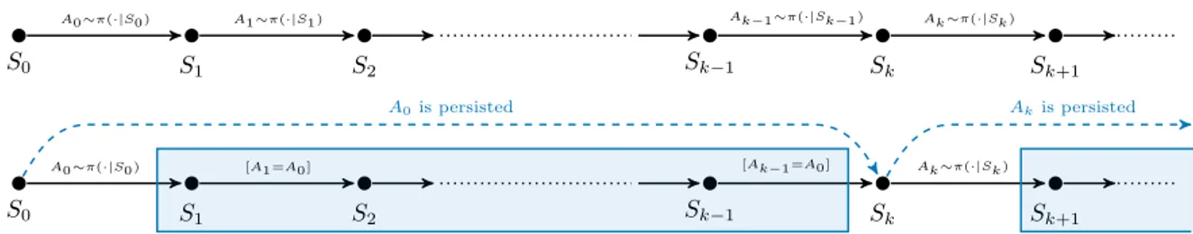
4.1 Agent-environment interaction without (top) and with (bottom) action persistence, highlighting duality. The transition generated by the k-persistent MDP _Mk is the cyan dashed arrow, while the

actions played by the k-persistent policies are inside the cyan rectangle. 23

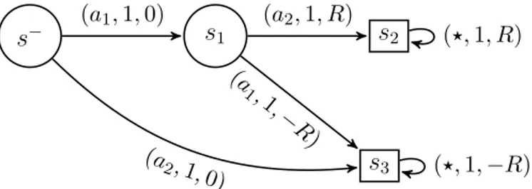
5.1 The MDP counter-example of Proposition 5.1.1, where R ą 0. Each arrow connecting two states s and s1 _{is labeled with the}

3-tuple pa, P ps1_{|s, aq, rps, aqq; the symbol ‹ denotes any action in} _A.

While the optimal policy in the original MDP starting in s´ _can

avoid negative rewards by executing an action sequence of the kind pa1, a2, . . . q, every policy in the k-persistent MDP, with k P Ně2,

inevitably ends in the negative terminal state, as the only possible action sequences are of the kind pa1, a1, . . . q and pa2, a2, . . . q. . . 29

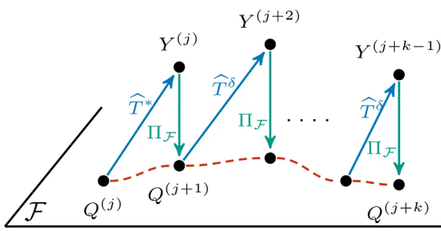
6.1 Illustration of PFQI(k) executed in the base MDP_{M1. The ˆ}T are the approximate Bellman Operators, subject to estimation error due to the finite dataset. Y are the estimates produced by ˆT . Our regressor belongs to the functional space_{F, so, when we fit it with} Y , we make a projection ΠF, i.e., we find the regressor in F, that

minimize the distance from Y . As you can see, we apply the operator ˆ

T˚ _{followed by ˆ}_Tδ _{for k ´ 1 times, in order to apply a Persistent}

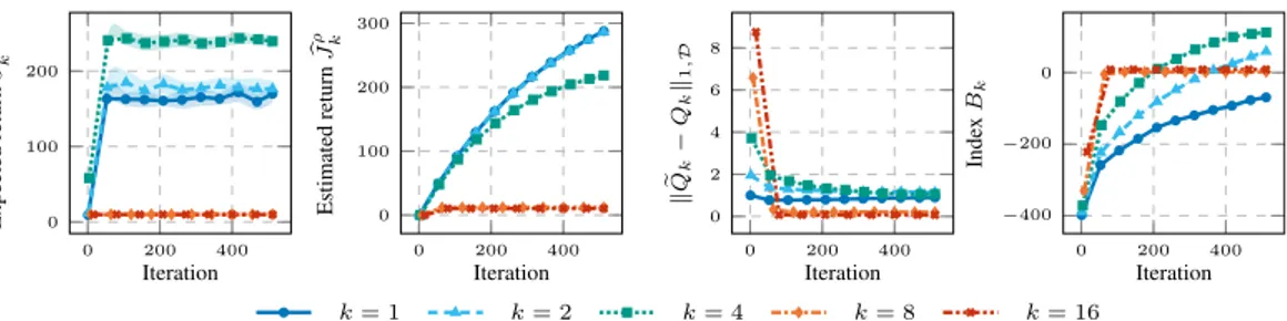
Bellman Operator. . . 47 7.1 Expected return pJρ,πk

k , estimated return pJ ρ

k, estimated expected

Bellman residual } rQk´ Qk}1,D, and persistence selection index Bk

in the Cartpole experiment as a function of the number of iterations for different persistences. 20 runs, 95 % c.i. . . 63

(9)

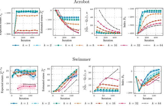
7.2 Each environment displays four different plots, all showing an index as a function of the number of iterations, using different colors and symbols for each persistence value. In the first plot, we show the expected return pJρ,πk

k , the average return obtained after collecting

ten trajectories with the policy πk, obtained by PFQI(k). In the

second plot, we can observe the estimated return pJ_kρ, obtained by averaging the Q-function Qk learned by PFQI(k), over the initial

states sampled from ρ. In the third plot, we can see the estimated expected Bellman residual } rQk ´ Qk}1,D. In the fourth plot, we

show the persistence selection index Bk, obtained combining the

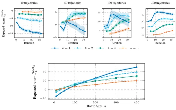
second and the third plot. For every environment, PFQI(k) has been executed 20 times, here we report the average results with a 95 % c.i. 67 7.3 The upper plots show the performances for each persistence along

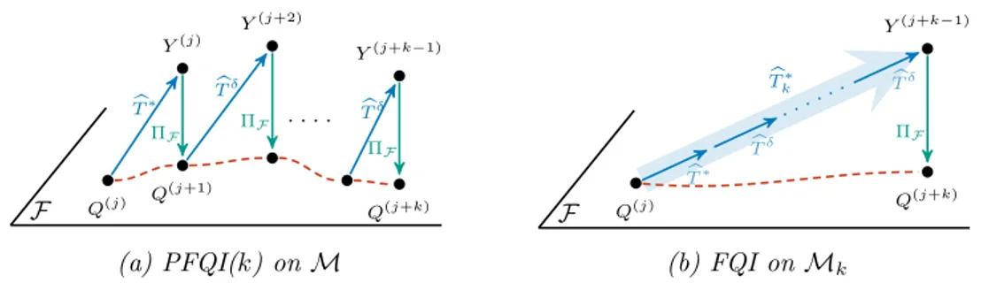
the iterations, with different numbers of trajectories. The plot below shows how performance at the last iteration (32) changes by varying the batch size. The plot is obtained interpolating results from experiments with different batch sizes: 10, 30, 50, 100, 200, 300, 400. 10 runs, 95% c.i. . . 69 8.1 Illustration of (a) PFQI(k) executed in the base MDP_{M and (b)}

the standard FQI executed in the k-persistent MDP_Mk. When we

work in (a), we apply ˆT˚ _{followed by ˆ}_Tδ _{for k ´ 1 times, so we need}

k iterations of PFQI(k) to apply a Persistent Bellman Operator and learn the effect of a k–persistent action. In (b) we work in_Mk, so 1

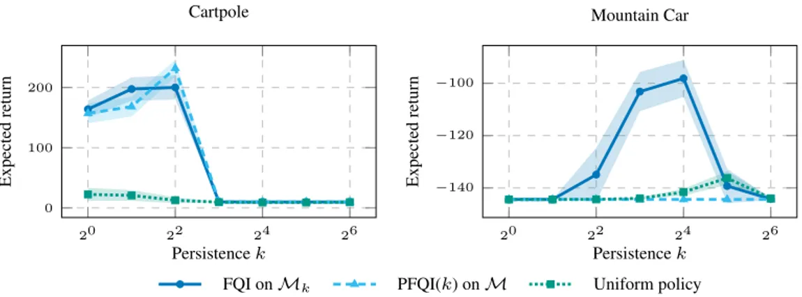
iteration of FQI is sufficient to learn the effect of a k–persistent action. 72 8.2 Performance of the policies learned with FQI on_Mk, PFQI(k) on

M and the one of the uniform policies for different values of the persistence k PK. 10 runs. 95% c.i. . . 73 8.3 Performance of the policies πk for k P K comparing when they

are executed in_Mk and when they are executed in Mpk1_q˚, where

(10)

List of Tables

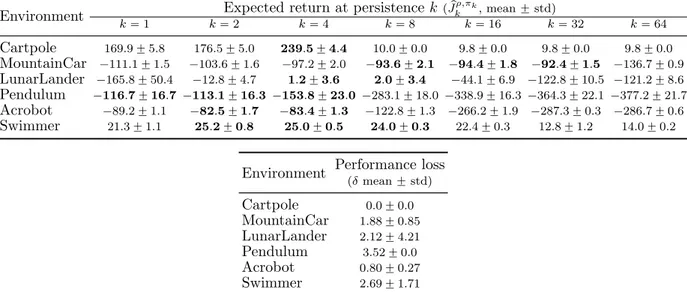
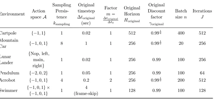
7.1 Results of PFQI execution in different environments and persistences. For each persistence k, we run PFQI for 20 times and we report the sample mean and the standard deviation of the estimated return of the last policy pJρ,πk

k , where each of the 20 estimated returns is

obtained by averaging 10 returns obtained evaluating the final policy learned starting from the state distribution ρ. For each environment, the group of best persistences that show not statistically significantly different performance (Welch’s t-test with p ă 0.05) are in bold. The last column reports the mean and the standard deviation of the performance loss δ between the optimal persistence and the one selected by the index Bk (Equation (6.6)). . . 62

7.2 Parameters of the experimental setting, used for the PFQI(k) exper-iments. . . 65 8.1 Results of PFQI execution of the policy πk learned with the k–

persistent operator in the k1_{–persistent MDP}_M

k1 in the Cartpole

experiment. For each k, we report the sample mean and the standard deviation of the estimated return of the last policy pJρ,πk

k1 . For each k,

the persistences k1 _{that show not statistically significantly different}

(11)

Abstract

The thesis is related to Batch Reinforcement Learning. Our purpose is to analyze how control frequency influences learning in this setting. In order to do so, we introduce the notion of action persistence that consists in the repetition of an action for a fixed number of decision steps, having the effect of modifying the control frequency. We start analyzing how action persistence affects the performance of the optimal policy, providing mathematical bounds that motivate the research of an ideal control frequency. Then we present a way to train agents with different control frequencies, proposing a novel algorithm, Persistent Fitted Q-Iteration (PFQI), that extends FQI, with the goal of learning the optimal value function at a given persistence. Finally, we proposed a heuristic approach to identify the optimal persistence from a set used in PFQI and present an experimental campaign on benchmark domains to show the advantages of action persistence and proving the effectiveness of our persistence selection method.

Keywords: Reinforcement Learning, Batch, Persistence, Control Frequency, FQI, PFQI

(12)

Estratto in Lingua Italiana

La tesi si colloca nell’ambito dell’Apprendimento per Rinforzo, Reinforcement Learning in inglese, un settore specifico dell’Apprendimento Automatico, Machine Learning in

inglese (RL, Sutton and Barto, 2018), che `e a sua volta una branca del vasto mondo

dell’intelligenza artificiale. Con Apprendimento per Rinforzo si intende un insieme di tecniche finalizzate a risolvere problemi caratterizzati dalla presenza di un agente che deve prendere azioni all’interno di un ambiente, che riceve una ricompensa in base alle azioni intraprese e che si pone l’obiettivo finale di massimizzare tale nozione di ricompensa.

Tipicamente il modello matematico impiegato per descrivere questo tipo di problemi `e il

Processo Decisionale di Markov (Puterman, 2014), in inglese Markov Decision Process (MDP).

L’uso di questo modello `e giustificato dal fatto che gran parte degli algoritmi relativi

all’Apprendimento per Rinforzo derivano dalla Programmazione Dinamica (Bertsekas, 2005), un insieme di tecniche che impiegano spesso il Processo Decisionale di Markov e che affrontano un problema complesso scomponendolo in sottoproblemi da risolvere in maniera ricorsiva. Diversamente dalla Programmazione Dinamica, l’Apprendimento per

Rinforzo non assume conoscenza del modello matematico esatto dell’MDP ed `e in grado

di risolvere MDP dove i metodi esatti divengono impraticabili.

La nostra attenzione si rivolger`a in particolare all’Apprendimento per Rinforzo offline

di tipo batch (Lange et al., 2012), un contesto in cui l’insieme dei dati raccolti sull’ambiente sono forniti interamente all’inizio, prima di poter applicare i relativi algoritmi. L’obiettivo dunque consiste nel trovare una politica di azione ottima, che massimizzi le ricompense accumulate, dato questo insieme di dati fissato. Una delle tecniche largamente impiegate

in questo contesto e derivante dalla programmazione dinamica, `e la tecnica denominata

Value Iteration. Tale tecnica cerca di calcolare laQ function ottima di un MDP attraverso

l’applicazione ripetuta dell’operatore di Bellman ottimo. La Q function ottima descrive il valore della ricompensa cumulata ottenuta eseguendo una certa azione in un determinato stato dell’MDP, presupponendo di compiere in futuro una sequenza di scelte ottime

per massimizzare la ricompensa totale accumulata. L’operatore di Bellman ottimo `e

(13)

fino ad arrivare ad un punto fisso. Pu`o essere impiegato in modo esatto, se abbiamo una conoscenza completa dell’MDP, o approssimato, se abbiamo a disposizione un numero limitato di dati raccolti nell’MDP.

L’obiettivo della tesi consiste nell’analizzare come la frequenza di controllo influenza l’apprendimento nel contesto dell’Apprendimento per Rinforzo offline di tipo batch. Per conseguire questo risultato, introduciamo il concetto di persistenza delle azioni, che consiste nella ripetizione di una certa azione per un numero prefissato di passi decisionali, con l’effetto risultante di modificare la frequenza di controllo. Questo ci permette di dare

nuove definizioni: quella di MDP persistito a persistenzak, costruito da un MDP di base,

in cui una transizione riassume in s`e una sequenza di k transizioni in cui si ripete sempre

la stessa azione, e la definizione di politica a persistenzak, politica di scelta delle azioni

che ripete la stessa scelta per k passi, prima di assumere una nuova decisione. Inoltre

viene formalizzato il concetto di Operatore di Bellman Persisito di valorek, che consente

il calcolo dellaQ function per gli stati di un MDP in cui le azioni vengono ripetute per k

passi consecutivi.

Da un punto di vista intuitivo, avere una frequenza di controllo pi`u fine dovrebbe

incrementare le performance dell’agente, visto che si ottiene una maggiore capacit`a di

controllo. Questo potrebbe portarci a pensare che la strategia per ottenere i risultati

migliori sia quella di controllare il sistema con la pi`u alta frequenza possibile, entro i

limiti fisici. Nonostante ci`o, nell’Apprendimento per Rinforzo la dinamica dell’ambiente

non `e nota e sono necessari dati per dedurla, dunque, una discretizzazione temporale

troppo fine potrebbe ottenere un risultato negativo, perch´e si rende il problema pi`u

complesso e difficile da risolvere.

Da un punto di vista teorico, analizziamo come la persistenza delle azioni influisce sulla performance della politica ottima, fornendo delle disuguaglianze matematiche che motivano la ricerca di una frequenza di controllo ideale. In primo luogo, si mette in luce con un MDP illustrativo, come la possibile perdita di performance causata dall’aumento di valore della persistenza sia limitata da un termine proporzionale al valore assoluto di

ricompensa massima che si pu`o ottenere in tale MDP. Successivamente, vengono forniti

bound matematici che catturano la perdita di performance causata dall’aumento del valore

di persistenza delle azioni, per quanto riguarda la distanza fra laQ function dell’MDP a

persistenza 1 e a persistenza k. Possiamo osservare una perdita pi`u contenuta quando

assumiamo la validit`a di propriet`a Lipschitz negli MDP (Rachelson and Lagoudakis, 2010;

Pirotta et al., 2015), propriet`a che descrivono un ambiente in cui stati simili presentano

caratteristiche simili e azioni simili hanno conseguenze simili se applicate in stati fra loro somiglianti. Nel corso di questa trattazione, risulta necessario introdurre anche un

nuovo concetto di continuit`a Lipschitz non presente in letteratura, la continuit`a Lipschitz

nel tempo, che garantisce un’evoluzione limitata dello stato a seguito di una transizione nell’MDP.

(14)

In seguito, presentiamo un metodo per addestrare agenti utilizzando diverse frequenze di controllo, proponendo un nuovo algoritmo, Persistent Fitted Q-Iteration (PFQI), estensione di Fitted Q-Iteration (FQI, Ernst et al., 2005). FQI calcola un’approssimazione della politica ottima da impiegare in un certo MDP, sfruttando un insieme di informazioni

raccolte su tale MDP. `E un algoritmo batch e offline che lavora sfruttando il principio

alla base di Value Iteration, che consiste quindi nell’applicazione iterativa dell’operatore

di Bellman ottimo per calcolare la Q function ottima dell’MDP. Questo consente di

formulare come output una politica che segue tale funzione in modo greedy, ovvero che sceglie sempre l’azione che porta verso ricompense maggiori secondo la funzione appresa.

PFQI, si pone invece l’obiettivo di imparare laQ function ottima di un MDP, ma sapendo

di agire con un certo valore di persistenza prestabilito. La principale differenza fra PFQI ed FQI consiste nell’impiego dell’operatore di Bellman ottimo persistito introdotto in

questo lavoro, piuttosto che l’operatore di Bellman ottimo tradizionale. Le propriet`a

teoriche di tale algoritmo ci motivano ad applicare valori persistenza maggiori di 1. Esse

ci permettono di comprendere che, più alta è la persistenza, più facile sarà approssimare

la Q function ottima degli MDP a quella persistenza. Ci`o permette alle politiche di

scegliere azioni con una conoscenza pi`u accurata del problema e ci fa intuire l’esistenza

di un valore ideale di persistenza, che ottimizza il compromesso fra la perdita dettata da un minor potere di controllo e il guadagno che si ottiene nell’approssimare una funzione

pi`u semplice.

Sono stati dunque presentati esperimenti in cui l’algoritmo PFQI viene applicato

in diversi ambienti offerti dalla libreria open source OpenAI gym. `E stato possibile

individuare come in certi contesti e con determinati parametri, l’utilizzo di valori di

persistenza maggiori di 1 risulta pi`u vantaggioso, superando quindi i risultati ottenuti

dell’algoritmo gi`a esistente FQI, che altro non `e che PFQI operato a persistenza 1. Viene

inoltre presentato un problema di tipo finanziario, che ci permette di mettere in luce come

la quantit`a di dati che abbiamo a disposizione risulti fundamentale nel determinare quale

sia la persistenza migliore con cui eseguire PFQI. Per farlo abbiamo provato a risolvere

tale problema fornendo in input datset di diversa dimensione. Si pu`o osservare dunque

che quando abbiamo pochi campioni, le persistenze pi`u alte risultano pi`u performanti,

mentre quelle pi`u basse risultano vincenti solo se abbiamo un numero sufficiente di dati.

Ci siamo inoltre posti un altro problema relativo al contesto batch e offline, nel quale si trova ad operare l’algoritmo che abbiamo proposto. Spesso in tali situazioni

non `e possibile valutare le politiche imparate dagli algoritmi testandole direttamente

sull’ambiente, perch´e i dati vengono raccolti interamente all’inizio e sono elaborati

solo successivamente. Quindi potrebbe venire a mancare la possibilit`a di testare in

futuro sul campo le politiche apprese in questo modo. Abbiamo dunque ricercato

un approcio euristico per individuare la politica ottima fra quelle imparate da PFQI usando vari livelli di persistenza. Questa scelta si basa su un indice costruito seguendo

(15)

opportune linee guida teoriche, che suggeriscono di combinare laQ function degli stati

iniziali dell’MDP e il Bellman residual. LaQ function degli stati iniziali cattura quanto

grande sar`a la ricompensa cumulata partendo dagli stati iniziali; il residuo di Bellman

consiste nella differenza fra laQ function e il valore ottenuto applicando l’operatore di

Bellman persistito a tale funzione, andando a catturare la qualit`a dell’approssimazione.

Dimostriamo inoltre l’efficacia di tale criterio testandolo sugli esperimenti effettuati con PFQI descritti precedentemente.

Nel corso delle nostre ricerce ci siamo inoltre imbattuti in altre questioni legate al tema della persistenza delle azioni. Ad esempio ci siamo accorti che durante la raccolta dei campioni preliminare all’esecuzione di algoritmi come FQI o PFQI, la politica

impiegata, che spesso `e una politica casuale uniforme sulle azioni, pu`o eventualmente essere

applicata con valori di persistenza maggiori di 1. Si pu`o osservare come in certi ambienti,

il mantenimento di un’azione per pi`u passi temporali consecutivi sia determinante

nell’esplorare lo spazio a sufficienza e nell’ottenere un insieme di dati sufficientemente

informativo. Un tema che dunque si potrebbe indagare ulteriormente `e come il valore

della persistenza della politica di esplorazione possa influire sull’apprendimento realizzato dagli algoritmi di Apprendimento per Rinforzo.

Un ultimo tipo di esperimenti degno di nota riguarda l’utilizzo delle politiche apprese

dall’algoritmo PFQI con persistenza k. Si pu`o osservare nell’ambiente Cartpole (Barto

et al., 1983), un ambiente offerto dalla libreria OpenAI gym, che le politiche imparate per

ripetere le azioni perk passi consecutivi, funzionano in modo pi`u efficace se utilizzate con

frequenza di controllo pi`u elevata, quindi persistendo le azioni un numero di voltek1_{ă k.}

Questo sembra essere spiegato dal fatto che l’apprendimento con una persistenza elevata

richiede di dover approssimare una Q function ottima pi`u semplice, e che l’impiego di

una politica con una persistenza pi`u bassa in fase applicativa introduce i benefici della

maggior capacit`a di controllo. Questo `e un altro tema che potrebbe essere ulteriormente

indagato e approfondito e che viene semplicemente introdotto.

Modellare la diversa frequenza di controllo tramite la persistenza delle azioni, `e un

tentativo di affrontare all’interno dell’Apprendimento per Rinforzo un problema, che gi`a

`e stato affrontato in letteratura tramite modelli come i Processi Decisionali Semi Markov

(Bradtke and Duff, 1994) e il concetto di Opzioni (Precup, 2001). I modelli precedenti sono molto generali e possono includere nella loro rappresentazione la descrizione del concetto di azione persistita, tuttavia questa nuova proposta risulta semplice e comoda

per rappresentare in modo pi`u specifico la frequenza di controllo, trarre risultati teorici e

formulare algoritmi.

Diverse sono ancora le domande aperte e le possibilit`a di applicare l’idea di persistenza.

Un esempio `e la trattazione degli algoritmi online, che vengono in questo lavoro totalmente

trascurati. Ci si augura dunque che il concetto di azione persistita porter`a a sviluppi

(16)

(17)

Chapter 1 Introduction

The thesis concerns the artificial intelligence field of reinforcement learning (RL, Sutton and Barto, 2018), an area of machine learning related on how agents ought to take actions in an environment so that they maximize a reward, which depends on the result of the actions performed and can be accumulated over time. The mathematical framework employed to describe an environment is typically a Markov decision process (MDP, Puterman, 2014), a discrete–time stochastic control process, that models a decision– making problem, where the outcomes of the actions are chosen by the decision-maker are

affected by uncertainty. The process is always in some states, and the decision–maker

may choose any actiona that is available in state s, each time step. At the next time step,

the process will move into a new state s1 _{obtaining a corresponding reward}_{r, according}

to a transition probability model.

MDPs have been already used in dynamic programming (Bertsekas, 2005), a set of techniques simplifying a complicated problem by breaking it down into simpler sub-problems in a recursive manner. Reinforcement learning and dynamic programming attempt to solve MDPs, by finding the optimal policy to execute, but they differ from each other, because reinforcement learning does not assume knowledge of an exact mathematical model of the MDP and targets large MDPs where exact methods, like dynamic programming techniques, become infeasible.

We focus on batch reinforcement learning (Lange et al., 2012), a specific setting, where the complete amount of learning experience, usually characterized by a set of transitions sampled from the system, is given a priori and is fixed. The task of the learning agent is then to derive a solution out of this given batch of samples, i.e., deriving an optimal policy that maximizes the cumulative reward. In particular we analyze and test Fitted Q-Iteration (FQI, Ernst et al., 2005), an algorithm that can be viewed as an approximate value iteration applied to action-value functions. In order to collect samples in a batch RL context we can generate trajectories, i.e., we start from an initial state

(18)

s0 and then follow a certain policy, allowing us to explore new states and observing the

corresponding reward. In this way, we can collect the tuples (s, a, r, s1_, _absorbing),

where s is the current state, a is the action performed, s1 _{is the new state reached,} _{r is}

the reward obtained andabsorbing indicates if s1 _{is absorbing i.e., a state indicating that}

the episode is terminated.

1.1 Motivations and Goals

The purpose of the thesis is understanding how the control frequency can influence performance in the context of batch reinforcement learning, and we focus on continuous-time environments and their discrete-continuous-time formulation.

We introduce the notion of action persistence that consists in the repetition of an action for a fixed number of decision steps, having the effect of modifying the control frequency. The idea of repeating actions has been previously heuristically employed in RL coped with deep RL architectures (Lakshminarayanan et al., 2017).

Intuitively, increasing the control frequency of the system offers the agent more control opportunities, possibly leading to improved performance as the agent has access to a larger policy space, the set of all agent’s strategies. This might wrongly suggest that we should control the system with the highest frequency possible, within its physical limits, in order to obtain better performance. However, in the RL framework, the environment dynamics is unknown, thus, a too fine discretization could result in the opposite effect, making the problem harder to solve. Indeed, any RL algorithm needs samples to figure out (implicitly or explicitly) how the environment evolves as an effect of the agent’s actions.

An interesting effect of modifying the control frequency can be noticed in the variation of the advantage function of state-action pairs (s, a), whose value indicates the benefit of

using the action a in a certain state s with respect to using the the action prescribed by

the policy in the same state. Indeed, when increasing the control frequency, the advantage of individual actions becomes infinitesimal, making them almost indistinguishable for standard value-based RL approaches (Tallec et al., 2019). As a consequence, the sample complexity increases, i.e., we need more training-samples in order to make an algorithm successfully learn the optimal policy. Instead, low frequencies allow the environment to evolve longer, making the effect of individual actions more easily detectable. Furthermore, in the presence of a system characterized by a “slowly evolving” dynamics, the gain obtained by increasing the control frequency might become negligible. Finally, in robotics, lower frequencies help to overcome some partial observability issues, like action execution delays (Kober and Peters, 2014).

Therefore, we experience a fundamental trade–off in the control frequency choice that involves the policy space (larger at high–frequency) and the sample complexity

(19)

(smaller at low–frequency). Thus, it seems natural to wonder: “what is the optimal control frequency? ” An answer to this question can disregard neither the task we are facing nor the learning algorithm we intend to employ. Indeed, the performance loss we experience by reducing the control frequency depends strictly on the properties of the system and, thus, of the task. Similarly, the dependence of the sample complexity on the control frequency is related to how the learning algorithm will employ the collected samples.

1.2 Contributions

The contributions of this thesis are theoretical, algorithmic and experimental. We first prove that action persistence can be represented by a suitable modification of the Bellman operators, which preserves the contraction property and, consequently, allows deriving the corresponding value functions.

We start analyzing how action persistence affects the performance from a theoretical point of view, providing an algorithm-independent bound, stating how much we can lose by decreasing the control frequency, given Lipschitz assumptions on the MDP. Then we present another mathematical bound, working in the context of approximate value and policy iteration, that states how much we can gain by decreasing the control frequency. The results related to the latter bound are the reasons why we focus on batch reinforcement learning and on FQI, an algorithm working in the context of approximate value iteration.

The theoretical results previously mentioned help us understanding that if we work on MDP with Lipschitz properties, using approximate value or policy iteration, we can hurt performance by employing too low or too high control frequencies. These two bounds combined highlight the trade off between sample complexity and policy space due to action persistence.

We assume to have access to a discrete–time MDP M∆t0, called base MDP, which is

obtained from the time discretization of a continuous–time MDP with fixed base control

time step ∆t0, or equivalently, a control frequency equal to f0 “ _∆t1₀. In this setting,

we want to select a suitable control time step ∆t that is an integer multiple of the base

time step ∆t0, i.e., ∆t “ k∆t0 with k P Ně1.1 Any choice ofk generates an MDP Mk∆t0

obtained from the base one_M∆t0 by altering the transition model so that each action is

repeated for k times. For this reason, we refer to k as the action persistence, i.e., the

1_{We are considering the near–continuous setting. This is almost w.l.o.g. compared to the}

continuous time since the discretization time step ∆t0 can be chosen to be arbitrarily small.

Typically, a lower bound on ∆t0 is imposed by the physical limitations of the system. Thus,

we restrict the search of ∆t from the continuous set Rą0 to the discrete set tk∆t0, k P Ně1u.

(20)

number of decision epochs in which an action is kept fixed. It is possible to appreciate the

same effect in the base MDP _M∆t0 by executing a (non-Markovian and non-stationary)

policy that persists every action for k time steps, i.e., a policy that chooses a new action

every k steps, otherwise repeats the previous action performed. In the first case we have

an MDPMk∆t0, displaying just the states reached every k steps. In the second case we

have a policy repeating an action for k steps, before choosing a new one, on an MDP

M∆t0. It can be easly noted that these are two formal methods describing the same

process.

Thanks to the concept of action persistence, we can formulate a novel algorithm, Persistent Fitted Q-Iteration (PFQI), an extension FQI, that, given a certain persistence k and samples taken at persistence 1, aim at learning the optimal value function of a

policy executing at persistence k, i.e., a policy that repeats the same action for k steps

before choosing a new action.

We provide also a heuristic approach to identify the optimal persistence, given a set of persistences used as input of the PFQI algorithm. In order to do so, we formulate a mathematical bound on the performance of the learned policy and an approximation of it, so that we can use it in practice to choose the best persistence level.

Then, we present an experimental campaign on benchmark domains to show the advantages of action persistence. In particular we analyze some OpenAI Gym environ-ments. For each one of them we collect a batch of trajectories, using them to perform PFQI, with a suitable selected range of persistence values. In this way, we obtain various policies working at different persistence levels. We evaluate these policies, observing that the best one is not always the one operating with the highest control frequency. Furthermore, we employ our persistence selection method, proving its effectiveness in choosing a good policy between the ones trained by PFQI. This is a useful tool in case we have not the opportunity to test the trained policies.

Finally we discuss about other topics emerged during our research and other exper-imental results obtained, leaving open questions that can be further deepened in the future.

1.3 Thesis Structure

The thesis is structured as follows.

In Chapter 2, some preliminary concepts needed to understand the rest of the thesis are discussed. In particular, we will focus on Markov Decision Processes, Reinforcement Learning, and the Fitted Q-Iteration algorithm.

(21)

thesis. Various ways of dealing with time control are discussed, in particular, how to treat continuous time and the concept of Temporal Abstraction.

In Chapter 4, the mathematical framework related to persisting action in MPDs

will be illustrated. We will explain how to formalize the k-persistent MDP and the

k-persistent policy. Finally the Persistent Bellman Operators will be introduced and analyzed.

In Chapter 5, we try to understand how much we lose by reducing the control frequency of our system. First of all, we analyze a toy MDP that makes us aware of how performance can be arbitrarily damaged by increasing the action persistence level. For that reason, we assume to work under Lipschitz conditions on the MDP, providing a mathematical bound on the performance loss due to the increased action persistence level.

In Chapter 6, the Persistent Fitted Q-Iteration (PFQI) algorithm will be showed, together with a theoretical analysis about computational complexity. Then, we discuss how error propagation works in this algorithm and approximate value and policy iteration in general. In this way we can show the advantage of using higher persistence levels in

estimating the Q˚

k, i.e., the Q function of the optimal policy working at persistence k.

So, to motivate the research of an ideal persistence level. Finally a persistence selection algorithm will be described. The algorithm works on the policies trained with PFQI with different persisitence levels, trying to output the best policy without testing them.

In Chapter 7, experimental results will be shown. PFQI is tested in various environ-ments, showing the existence of “ideal” persistence levels. Furthermore the persistence selection method will be tested showing its effectiveness.

In Chapter 8, some open questions will be tackled and introduced. In particular we

show what happens by performing FQI on MDPs of the kind Mk∆t0, observing how

higher persistence levels can be beneficial for performance. Then we discuss with an

example what happen in PFQI, if we train a policy with persistence k and execute it

with a different persistence levelk1_{. Finally we summarize the purposes of the thesis, the}

(22)

Chapter 2 Preliminaries

This chapter provides the necessary background to understand the content of the thesis. In Section 2.1, we start providing preliminary mathematical definitions for probability space, norm, function spaces, Lipschitz continuity and Kantorivich distance. After that, in Section 2.2, we formalize the decision making problems, introducing the mathematical framework of Markov decision processes (MDP) in Section 2.2.1, and afterwards, the related concepts of policy (Section 2.2.2), value functions (Section 2.2.3) and Bellman operators (Section 2.2.4). Then, we introduce dynamic programming (DP)-based and reinforcement learning (RL) planning problems in Section 2.3. We introduce batch re-inforcement learning in Section 2.3.2. We describe the value-based approach to solve RL/Planning problems in Section 2.3.3 and review methods such as value iteration and policy iteration algorithms, and how to deal with large state spaces using function ap-proximation. Then, in Section 2.3.4, we show a common way to measure the performance of RL algorithms. Finally, in Section 2.4.1, a state-of-the-art algorithm in the family of Batch Reinforcement Learning, Fitted Q-Iteration, will be described. All theoretical analysis that will be investigated in the next chapters can be applied to this algorithm and the new one proposed, PFQI, which is an extension of the first one.

There are textbooks and monographs on RL and Planning that provide exhaustive explaination of these topics and their associated algorithms. For instance, Sutton and Barto (2018) is a textbook covering both RL and Planning at an introductory level, with more emphasis on the learning aspects. Sutton and Barto consider both discrete and continuous state spaces. Another important textbook in the RL literature is made by Szepesvari (2009), a shorter book illustrating the major ideas underlying state-of-the-art RL algorithms.

(23)

2.1 Preliminary Concepts

In this section, we will present the notation and the basic notions that we will employ in the remainder of the thesis.

2.1.1 Probability Space

Let’s define _{X a set and σ}X is the σ-algebra over X , i.e., a collection of subsets of X

that includes X itself, that is closed under complement, and is closed under countable

unions. Then, we define PpX q, the set of all probability measures over pX , σXq. BpX )

is the space of bounded measurable functions with respect to pX , σXq andBpX , Lq is

the space of bounded measurable functions with bound 0 ă L ă 1. If x P_{X , we denote}

with δx the Dirac measure defined on x.

Given two σ-finite measures v1 and v2 on some measurable space pX , σXq, v1 is

absolutely continuous w.r.t. v2 if there is a non-negative measurable function f :X Ñ R

such that v1pAq “ ş fdv2 for all A P σX. Moreover, we know that v1 is absolutely

continuous w.r.t. v2 if and only if v1! v2, i.e.,v2pAq “ 0 implies that v1pAq “ 0. Finally,

we say that dv1

dv2 “ f is the Radon-Nikodym derivative of v1 w.r.t. v2 (Rosenthal, 2006).

2.1.2 Norm and Function Spaces

Let’s define ρ PPpX q a probability measure and f P BpX q a measurable function. We

abbreviateρf “ş_Xf pxqρpdxq. We say that the Lppρq-norm is defined as:

}f }p_p,ρ “ ż

X

|f pxq|pρpdxq,

forp ě 1, while the L8-norm is defined as:

}f }₈ “ sup

xPX

f pxq.

If we callD “ txiuni“1ĎX , the empirical norm Lppρq is:

}f }p_p,D “ 1 n n ÿ i“1 |f pxiq|p. We introduce ρ|f pxq|p

“ }f }p_p,ρ as a shorthand notation. Finally, we say that Πρ,B :

BpX q Ñ BpX q is the projection operator, defined as:

Πρ,BV fi arg min V1_P_{BpX q} › ›V1´ V › › 2 ρ, forV PBpX q.

(24)

2.1.3 Lipschitz Continuity

Here we introduce some notions about Lipschitz Continuity and distances between probability distributions. Lipschitz Continuity is a concept employed to describe a function that provides similar outputs given similar inputs. To be more specific, given two inputs, the distance between their images according to the function will be bounded by the distance between the two original inputs.

If we let pX , dXq and pY, dYq be two metric spaces, a function f :X Ñ Y is called

Lf-Lipschitz continuous (Lf-LC), whereLf ě 0, if for all x, x1 PX we have:

dYpf pxq, f px1qq ď LfdXpx, x1q. (2.1)

Moreover, we define the Lipschitz semi-norm as }f }_L“ supx,x1_{PX :x‰x}1 dYpf pxq,f px

1_qq

dXpx,x1_q . For

real functions we employ Euclidean distancedYpy, y1q “ }y ´ y1}₂; while for probability

distributions, we use the Kantorovich (L1-Wasserstein) metric. The Kantorovich distance

between two probability distributions can be seen as the minimum cost of moving probability mass, in order to transform one probability distribution into the other. The

Kantorovich (L1-Wasserstein) metric defined for µ, ν PPpZq as (Villani, 2008):

dYpµ, νq “W1pµ, νq “ sup f :}f }_Lď1 ˇ ˇ ˇ ˇ ż Z f pzqpµ ´ νqpdzq ˇ ˇ ˇ ˇ . (2.2)

2.2 Sequential Decision Making Problems

2.2.1 MDPs

A discrete-time Markov Decision Process (MDP, Puterman, 2014) is a 5-tuple _{M “}

pS, A, P, R, γq, where S is a measurable set of states, A is a measurable set of actions,

P :_{S ˆ A Ñ PpSq is the transition kernel that for each state-action pair ps, aq P S ˆ A}

provides the probability distributionP p¨|s, aq of the next state, R :S ˆ A Ñ PpRq is the

reward distributionRp¨|s, aq for performing action a PA in state s P S, whose expected

value is denoted byrps, aq “ş

RsRpds|s, aq and uniformly bounded by Rmaxă `8, and

γ P r0, 1q is the discount factor.

MDPs are a mathematical framework used to model a discrete-time evolution of a stochastic process, where an agent can take an action at each time step. The dynamical

system starts in a random initial state_S0 „ ρ where „ denotes thatS0 is drawn from

distribution ρ and the initial time step is usually t “ 0. At each time-step t, an action

AtPA is selected by the agent, following a policy π, so At„ πp¨|Stq, i.e., the action is

drown from a distributionπ, according to the current state S0. After having executed the

(25)

Rt is the reward that the agent receives at timet and St`1 is the state at timet ` 1. By

following this procedure we can obtain a trajectory pS0, A0, R0, S1, A1, R1, ...q.

The MDPs can be classified according to properties of the underlying state-space_S.

In case the state space_{S and the action space A are finite, we get a finite MDP. If we}

consider a measurable subset of Rd pS Ď Rdq, we get instead a continuous state-space

MDP.

2.2.2 Policy

A policy π “ pπtq_tPN is a sequence of functions πt : Ht Ñ PpAq mapping a history

Ht“ pS0, A0, ..., St´1, At´1, Stq of length t P Ně1 to a probability distribution over A,

where _Ht“ pS ˆ AqtˆS.

If for each t and Ht, the policyπt assigns mass one to a single point inA, π is called

deterministic (nonrandomized) policy; if it assigns a distribution over _{A, it is called}

stochastic or randomized policy.

If πt depends only on the last visited stateSt then it is called Markovian, i.e.,.

πt:S Ñ PpAq

Moreover, if πt does not depend on t it is stationary, in this case we remove the

subscriptt. We denote with Π the set of Markovian stationary policies.

A policyπ induces a (state-action) transition kernel Pπ _:_{S ˆ A Ñ PpS ˆ Aq, defined}

for any measurable setB Ď S ˆ A as (Farahmand, 2011):

pPπqpB|s, aq “ ż S P pds1 |s, aq ż A πpda1 |s1qδps1_,a1_qpBq. (2.3)

Where the dirac functionδps1_,a1_qpBq, describe a probability distribution where the couple

pa1, s1q has probability is 1 of being selected.

The m-step transition probability kernels pPπqm:_{S ˆ A Ñ PpS ˆ Aq for m “ 2, 3, ...}

are inductively defined as:

pPπqmpB|s, aq “

ż

S

P pds1

|s, aqpPπqm´1pB|s1, πps1qq. (2.4)

We can now define a right-linear operatorP ¨ :BpS ˆ Aq Ñ BpS ˆ Aq, given the

probability transition kernelsP :S ˆ A Ñ PpS ˆ Aq:

pP Qqps, aq “ ż

SˆA

P pds1_{, da}1

|s, aqQps1, a1q.

Similarly, we can define the left-linear operator ¨P :PpS ˆ Aq Ñ PpS ˆ Aq given a

probability measureρ PPpS ˆ Aq and a measurable subset B of S ˆ A:

pρP qpBq “

ż

ρpds, daqP pds1_{, a}1

(26)

2.2.3 Value functions

The action-value function, or Q-function, of a policyπ P Π is the expected discounted

sum of the rewards obtained by performing action a in state s and following policy π

thereafter: Qπps, aq “ E“ `8 ÿ t“0 γtRt|S0 “ s, A0 “ a‰,

where Rt„ Rp¨|St, Atq, St`1„ P p¨|St, Atq, and At`1„ πp¨|St`1q for all t P N. The

value function is the expectation of the Q-function over the actions:

Vπpsq “

ż

A

πpda|sqQπps, aq.

Given a distributionρ PPpSq, we define the expected return as:

Jρ,πpsq “

ż

S

ρpdsqVπpsq.

The optimal Q-function is given by:

Q˚

ps, aq “ sup

πPΠ

Qπps, aq.

for all ps, aq P_{S ˆ A.}

A policyπ is greedy w.r.t. a function f P BpS ˆ Aq if it plays only greedy actions,

i.e.,πp¨|sq PP parg max_aPAf ps, aqq. An optimal policy π˚

P Π is any policy greedy w.r.t.

Q˚ _{(Bertsekas and Shreve, 2004).}

2.2.4 Bellman Operators

Given a policyπ P Π, the Bellman Expectation Operator Tπ _:_{BpS ˆAq Ñ BpS ˆAq and}

the Bellman Optimal Operator T˚ _:BpS ˆ Aq Ñ BpS ˆ Aq are defined for a bounded

measurable function f PBpS ˆ Aq and ps, aq P S ˆ A as (Bertsekas and Shreve, 2004):

pTπf qps, aq “ rps, aq ` pPπf q ps, aq, pT˚f qps, aq “ rps, aq ` γ ż S P pds1 |s, aq max a1_PAf ps 1_{, a}1 q.

BothTπ _and_T˚ _are_{γ-contractions in L}

8-norm and, consequently, they have a unique

fixed point, that are the Q-function of policyπ (Tπ_Qπ

“ Qπ) and the optimal Q-function

(T˚_Q˚

“ Q˚) respectively.

If the action set is finite, the optimal value function can be attained by a deterministic Markov stationary policy. The same holds also for infinite action sets, whenever certain compactness conditions are satisfied (Bertsekas and Shreve, 2004).

(27)

2.3 Reinforcement Learning

The reinforcement learning problem consists in finding a policy π that displays a

perfor-mance equal or close to that of the optimal policy π˚_{. In this thesis, we only focus on}

problems that can be modeled by an MDP.

Differently from planning problems, where the transition probability kernel P p¨|s, aq

and the reward distribution_{Rp¨|s, aq of the MDP are known, in reinforcement learning}

eitherP or R or even both are not directly accessible. So, in order to collect information

aboutP orR, interacting with the MDP is necessary, i.e., we observe an agent, selecting

actionAt at state St, gettingRt„Rp.|St, Atq as a reward and going to a new state St`1

according to the transition probability kernel. As a result we can collect a trajectory, i.e., a sequence of states, actions and rewards encountered by the agent exploring the MDP,

pS0, A0, R0, S1, A1, R1, ...q. So, by observing samples of the distributions P and R, we

can infer how the MDP works.

There are other cases where RL approaches are needed, although we have more

information. For instance, we could not have information about the distributions

Rp.|s, aq and P p.|s, aq, but we can have access to a flexible data generator that gets

any ps, aq P_{S ˆ A as input and returns r „ Rp.|s, aq and s}1

„ P p.|s, aq. Sometimes we

know P p.|s, aq, nevertheless _{S displays a large cardinality, or is even infinite, making}

impractical the calculation ofTπ_{Q. Approximate Dynamic Programming is the name of}

the problem of finding a good policy in these scenarios.

There are two major classes of approaches to solve RL/Planning problems, Value Space Search and Policy Space Search. In this work, we only focus on the value-based approaches. The purpose of Value-based approaches is to find a good enough estimate

ˆ

Q (or ˆV ) of the optimal value function Q˚ _(or _V˚_{). By finding ˆ}_{Q (or ˆ}_{V ), the greedy}

policyπp.; ˆQq will be close to the optimal policy in some well-defined sense.

2.3.1 Online vs Offline Reinforcement Learning

In order to solve RL/Planning problems we need data, so, the process of collecting them is fundamental. There are two main categories to classify the data collection setting: online or offline.

If the trajectories pS1, A1, R1, ...q are generated during the learning phase, we are in

an online setting. That means it is possible to use different policies in different moments. If, instead, the agent is provided with a dataset, we are in an offline setting, because there is no control over how the data are generated. The dataset is usually in the form

Dn“ tpS1, A1, R1, S11q, ..., pSn, An, Rn, Sn1qu,

where Rt„ Rp¨|St, Atq, St`1„ P p¨|St, Atq, Ai „ πbp.|Siq, and Si„ νSpi “ 1, ..., nq, with

(28)

policy used to generate data, usually stochastic and unknown to the agent. Samples Si

and Si`1may be coupled through Si1“ Si`1, so they belong to the same trajectory, but

they can also be sampled independently.

In this work, we will illustrate only examples of offline data collection settings.

2.3.2 Batch vs Incremental Processing

In RL/Planning problems the data processing method can be categorized as batch or

incremental. In a batch process it is possible to access any element of the data set _Dn at

any time. In an incremental algorithm, instead, new data samples are available over time and the computation only depends on the most recent ones.

Which of these settings is preferred depends on the problem we need to solve. In case

we have an already collected dataset _Dn and the interaction with the MDP is impossible,

we are inevitably in the offline setting. In this context, we should be more inclined to use batch algorithms for data processing, because they are usually more data efficient, unless we have a limited computation time. In case we know the MDP or we can access to its generative model or our agent can act in the environment, we are facing an online data sampling scenario, so both batch and incremental algorithms may be used. In the remainder of the thesis, we focus on batch algorithms.

2.3.3 Value Based Approach

The purpose of value-based approaches for solving RL/Planning problems is to find the

fixed point (or some approximation of it) of the Bellman optimality operatorQ˚ _{“ T}˚_Q˚

(orV˚ _{“ T}˚_V˚_{) or , in case of policy evaluation, the fixed point of the Bellman operator}

Qπ

“ TπQπ (or Vπ

“ TπVπ).

In order to find a close to optimal value function, we need to find a way to represent

the action-value function Q (tabular representation). In case S ˆ A is a small finite

space, Q can be represented by a finite number of real values. When this is not the

case, we need to compute an approximation ofQ over the spaceS ˆ A, by means of an

approximant function, that approximate Q in a simpler way. That means we are resorting to Function Approximation (FA), a technique with interesting aspects to be discussed from the approximation theory point of view (Devore, 1998) and the statistical learning

theory point of view (Gy¨orfi et al., 2002).

Once we have a way to represent the action-value function Q, we need to know

how to evaluate Tπ_{Q or T}˚_{Q. Even though P p.|s, aq is known, the calculation is often}

intractable for large state spaces. A reasonable way to deal with it, is to approximately

estimate it by random sampling fromP p.|s, aq.

Finally, we have to find the fixed point of the Bellman operatorsTπ _and_T˚_{. There are}

(29)

Value Iteration and Policy Iteration, iterative procedures that make use of the contraction or monotonicity properties of the Bellman Operators. Different authors, like Bertsekas and Shreve (2004) and Szepesvari (1997b) detail the conditions that guarantee these methods to work.

In Value Iteration, the algorithm starts from an initial value function Q0 (or likewise

V0), and iteratively appliesT˚ (orTπ for the policy evaluation problem) to the previous

estimate:

Qk`1“ T˚Qk

We know that limkÑ8pT˚qkQ0“ Q˚and limkÑ8pTπqkQ0“ Qπ for everyQ0(Proposition

2.6 of Bertsekas and Tsitsiklis (1996) for the result for finite MDPs; Proposition 4.2(c) of Bertsekas and Shreve (2004) for a more general result).

There are some cases, in particular when the state-action space is large, where this procedure can only be performed in an approximate way:

Qk`1« T˚Qk

This procedure is called Approximate Value Iteration (AVI). There are various examples of AVI in literature, like tree-based Fitted Q-Iteration of (Ernst et al., 2005), multi-layer perceptron-based Fitted Q-Iteration of (Riedmiller, 2005), and Fitted Q-Iteration for continuous action spaces of (Antos et al., 2008). In Munos and Szepesvari (2008) it is possible to find more information on AVI.

Another iterative method to find the fixed point of the Bellman optimality operator is Policy Iteration (PI). This method consists in alternating two steps, called Policy Evaluation and Policy Improvement. The first step to apply is Policy Evaluation, which

consists in taking a policyπi, evaluating it and findingQπi, i.e., aQ function that satisfies

Tπi_Qπi _{“ Q}πi_{. Then, we apply Policy Improvement, i.e., we build the greedy policy}

w.r.t. the most recent value function πi`1 “ ˆπp.; Qπiq. By repeating these two steps

consecutively we generate a sequence of policies and their corresponding action-value functions:

Qπ0

Ñ π1 Ñ Qπ1 Ñ π2Ñ ...

It is known that after a finite number of iterations, if the policy evaluation step of PI is done exactly, PI yields the optimal policy for finite state/action MDPs. We also know from Bertsekas and Shreve (2004), that a slightly modified policy iteration algorithm, with the possibility of having certain amount of error during the policy evaluation step, still terminates in a finite number of iterations and the value of the resulting policy is close to the optimal one.

(30)

In case we deal with large problems, we can only solve the policy evaluation step in an approximate way, i.e., we need to resort to Approximate Policy Iteration (API), that is:

Qk« TkπQk (2.5)

One way to solve API is to use AVI, in order to find the fixed point of Tπ

k operator.

In Section 2.4.1 we illustrate Fitted Q-Iteration, an algorithm that resort to AVI in order to solve RL problems.

2.3.4 Performance Loss Measure

A common performance loss measure of RL/Planning algorithms is the Value Function error :

||V˚´ Vπ||p,ρ

In order to understand its meaning, let us consider a policy π which is the output of

an RL/Planning algorithm, such thatπ “ ˆπp.; ˆQq, i.e., π is the greedy policy w.r.t. an

estimated action-value function ˆQ. Now let us consider an agent starting at the initial

stateS “ s, following the policy π. Its expected return would be Vπ_{psq. If we want to}

compare Vπ

psq with V˚psq, which is the expected return following an optimal policy

starting from state s, we can just calculate the difference V˚_{psq ´ V}π

psq ě 0. Let us suppose instead, that the agent’s initial state is not fixed, but is distributed according

to the “performance measuring” distribution ρ PPpSq, that stresses the importance of

certain regions of the state space as the initial state of the trajectories generated by the agent. In such case, we should employ another performance loss measure. For instance, we

could use theL1pρq-norm between V˚psq and Vπpsq, to determine the expected difference

between the performance obtained by following policyπ instead of π˚_.

Up to now we always employed theL1-norm, but we could also use otherLp-norms

p1 ď p ď 1q. For instance, the L8-norm is another common choice, however, it often

outputs a too pessimistic value, because a large point-wise performance loss error can lead to a large performance loss overall, also in case it happens in a small subset of the state space.

Furthermore, it is also possible to define the performance loss w.r.t. the action-value

functions, i.e., ||Q˚

´ Qπ||p,ρ. In this case, the initial action-state is selected according to

ρ PPpS ˆ Aq. In this work, we focus on the action-value function error, employing the

(31)

Algorithm 1 Fitted Q-Iteration

Input: a regression algorithm andD “ tpsi, ai, s1i, riquni“1batch samples

Output: greedy policyπpjq

j “ 0

initialize Qp0q_{ps, aq with a default value}

while stopping conditions are not reached do j “ j ` 1

Build the training set_{T “ tpu}i, oiq, i “ 1, ..., nu based on the the function Qpj´1q

and on the full set of four-tuplesD:

ui “ psi, aiq, oi “ ri` γ max

¯ aPA Q

pj´1q

ps1i, ¯aq,

Use the regression algorithm to induce fromT the function Qpjq_.

end while πpjq

psq P arg maxaPAQpjqps, aq, @s PS

2.4 Fitted Q-Iteration

In this section, we introduce the Fitted Q-Iteration (FQI) (Ernst et al., 2005), an algorithm that computes an approximation of the optimal policy, using the information derived from a dataset. It is an example of a batch and offline algorithm, working under the principle of Value Iteration with Function Approximation. FQI and Persistent Fitted Q-Iteration (PFQI), the new algorithm proposed, are used during the experimental part of this thesis. This is the reason why we describe the details of FQI in Section 2.4.1.

In order to perform RL with Function Approximation, for instance using FQI and PFQI, we need a regressor. A regressor is a statistical model for estimating the rela-tionships between a dependent variable (often called the outcome variable) and one or more independent variables. A regressor can then be used to estimate the action-value

functionQps, aq, from an element of the state-action space ps, aq (s P_{S and a P A).}

During the experimental part of the thesis, FQI and PFQI algorithms employ a regressor from the family of the Random Forests, that we briefly introduce in Section 2.4.2.

2.4.1 The Algorithm

The fitted Q-Iteration (FQI) algorithm yields an approximation of the the

action-value functionQps, aq, corresponding to an infinite horizon optimal control problem with

(32)

horizon. FQI is an offline algorithm, that needs a dataset in the form: D “ tpsi, ai, s1i, riquni“1,

a set of n samples, representing the fact of having executed action ai in statesi, with

the result of reaching a new state s1

i and getting a rewardri.

The first iteration of FQI consists in estimating a Qp1q _{function, corresponding to a}

1-step optimization, which is the conditional expectation of the instantaneous rewardr

given the state-action pair ps, aq, so Qp1q_{ps, aq “ Err|S “ s, A “ as. We can approximate}

Qp1q _{by executing a (batch mode) regression algorithm to a training set with inputs}

tpsi, aiq, i “ 1, ..., nu and target outputs, ri pq1,i“ riq.

During the j-th iteration, a Qpjq _{function, corresponding to a j-step optimization}

horizon, is derived (using a batch mode regression algorithm). At this step, the function

Qpjq _{is obtained with the same regression algorithm used before, using the same inputs}

tpsi, aiq, i “ 1, ..., nu and the outputs derived from the the approximate Qpj´1q-function

returned at the previous step, by applying the empirical Bellman operator:

qj,i“ ri` γ max

¯ aPA Q

pj´1q

ps1i, ¯aq

whereγ P r0, 1q is the discount factor. This way of approximating the Qpjq _{function can}

be seen as a “value iteration” based strategy.

The algorithm iterates until a stopping condition is reached. This condition can be simply defined as the fact of having reached a maximum amount of iterations, specified a priori at the beginning of the algorithm. When the stopping conditions are met a greedy

policyπpjq _{is built from the final} _Qpjq _{function obtained:}

πpjq

psq P arg max

aPA

Qpjq

ps, aq, @s PS.

The pseudocode for FQI is illustrated in Algorithm 1. For more information on the FQI algorithm, further details can be found in Ernst et al. (2005).

2.4.2 Random Forests

Random forests are an ensemble learning method for classification (and regression) that operate by constructing a multitude of decision trees at training time and outputting the class that is the mode of the classes output by individual trees. The algorithm for inducing a random forest was developed by Leo Breiman and Adele Cutler, and “Random Forests” is their trademark (Breiman, 2001). The term came from random decision forests that was first proposed by Tin Kam Ho of Bell Labs in 1995 (Ho, 1995). The method combines Breiman’s bagging idea and the random selection of features, introduced

(33)

independently by Ho (Ho, 1995, 1997) and Amit and Geman (Amit, 1998) in order to construct a collection of decision trees with controlled variance.

The fundamental element of a Random Forest is the decision tree, a flowchart-like function, that receives as input a vector of features, and outputs a numerical value (regression) or a label (classification). Each internal node of the tree represent a “test” on an attribute (e.g., verify if a feature satisfies certain conditions), each branch represents the outcome of the test, leading to a new sub-tree and each leaf node represents the output.

The main Random Forest idea is to apply the ensamble technique of bagging (Breiman,

1994), to tree learners. We suppose to haveB decision trees to build and a training set

X “ x1, ..., xnwith responses Y “ y1, ..., yn. For each decision tree tb, we select a set of

random samples with replacement from the training set and fit the decision tree with such samples. A peculiar aspect of building the decision trees in Random Forests is that at each candidate split in the learning process, a random subset of the features is selected, instead of the most informative ones. For further details on how to fit decision trees, please refer to Chapter 3.4 of Mitchell (1997). Once we finished the training procedure,

predictions for unseen samples x1 _{can be made by averaging the predictions from all the}

individual regression trees onx1_:

ˆ y “ 1 B B ÿ b“1 tbpx1q

or by taking the majority vote in the case of classification tree. The strength of this bootstrapping procedure consists in decreasing the variance of the model, without increasing the bias. This means that the predictions of a single tree can be highly sensitive to noise in its training set, while the average of many trees is not, as long as the trees are not correlated.

Another similar regressor is the extremely randomized trees, or ExtraTrees (Geurts et al., 2006). They are still an ensamble of individual decision trees, but they differ from Random Forests for two aspects, i.e., each tree is trained using the whole learning sample (not just a bootstrap sample) and the splitting procedure of a node is randomized. Usually, the locally optimal cut-point for each feature under consideration is calculated, in ExtraTrees instead, for each feature, a random cut-point is selected from a uniform distribution within the feature’s empirical range. Then, the final split chosen from all the randomly generated splits, is the one that yields the highest score. This regressor is the one employed in FQI and PFQI during the experimental part this thesis.

(34)

Chapter 3 State Of The Art

In this chapter we will describe the state of the art related to the topic of the thesis, i.e., how control frequency influences learning in the context of reinforcement learning. An overview about previous researches will be given. In particular in Section 3.1 we show ways to deal with continuous time problems, in Section 3.2 we give a brief overview about Temporal Abstraction.

3.1 Continuous Time RL

In recent years, Reinforcement Learning (RL, Sutton and Barto, 2018) has proven to be a successful approach to address complex control tasks: from robotic locomotion (e.g., Peters and Schaal, 2008; Kober and Peters, 2014; Haarnoja et al., 2019; Kilinc et al., 2019) to continuous system control (e.g., Lillicrap et al., 2016; Schulman et al., 2015, 2017). These classes of problems are usually formalized in the framework of the discrete–time Markov Decision Processes (MDP, Puterman, 2014), assuming that the control signal is issued at discrete time instants. However, many relevant real–world problems are more naturally defined in the continuous–time domain (Luenberger, 1979). Even though a branch of literature has studied the application of RL to continuous–time MDPs Bradtke and Duff (1994); Munos and Bourgine (1997); Doya (2000), the majority of the research has focused on the discrete–time formulation, which appears to be a necessary, but effective, approximation.

3.1.1 Semi Markov Approach to Continuous Time

Among the first attempts to extend RL to the continuous–time domain, we find the work by Bradtke and Duff (1994) by means of the semi–Markov decision processes (Howard, 1963) for finite–state problems. According to this formalism we have to introduce into the

(35)

usual MDP a probability distributionF ps, s1

|aq, describing how much time occurs, when

transitioning from states to state s1 _{using action} _{a. The action persistence framework}

proposed in this thesis can be modeled according to this formulation, stating that we have

probability 1 of having actions lastingk ¨ ∆t, where ∆t is the time interval corresponding

to a step in the base MDPM, over which we execute a k–step persistent policy, a policy

repeating the same action fork steps before choosing a new one. Although this formalism

is more general, the action persistence framework is simpler to treat and allows us to state theoretical results about the effects of modifying the control frequency of the MDP.

3.1.2 Optimal Control

The optimal control literature has extensively studied the solution of the Hamilton-Jacobi-Bellman equation, i.e., the continuous–time counterpart of the Hamilton-Jacobi-Bellman equation, when assuming the knowledge of the environment dynamics (Bertsekas, 2005; Fleming and Soner, 2006). The Hamilton-Jacobi-Bellman equation gives a necessary and sufficient condition for optimality of a control with respect to a loss function. The model–free case has been tackled by resorting to time (and space) discretizations (Peterson, 1993), with also convergence guarantees (Munos, 1997; Munos and Bourgine, 1997), and coped with function approximation (Dayan and Singh, 1995; Doya, 2000).

3.1.3 Advantage Updating

The continuous–time domain is also addressed by advantage updating (Baird, 1994), in which Q–learning (Watkins, 1989) is modified to account for infinitesimal control timesteps. Q–learning is an online RL algorithm consisting in a value iteration update of

theQ function, the usual action value function defined in Section 2.2.3. Every time the

agent makes a step in the MDP, theQ function is iteratively updated in this way:

Qps, aqnew“ Qps, aqold` αpr ` γ max

¯ a Q

old

ps1, ¯aq ´ Qps, aqoldq,

where r is the instantaneous reward, s1 _{is the next state of}_{s, when taking action a, α is}

the learning rate andγ is the discount factor. The last two elements are opportunely

tuned parameters such that: α, γ P r0, 1q.

Instead of storing the Q–function, the advantage updating records the advantage function:

Aps, aq “ 1

∆trQps, aq ´ max¯a Qps, ¯aqs,

where Qps, aq is the usual action value function and ∆t is the time interval of the action

(36)

while Q–learning cannot, and learns faster than Q–learning in problems with small time steps or noise.

More recently, the sensitivity of deep RL algorithm to the time discretization has been analyzed in Tallec et al. (2019), showing that Q–learning fails, when working with infinitesimal time steps and proposing an adaptation of advantage updating to deal with small time scales, that can be employed with deep architecture. In particular, it is shown that approaches based on the estimation of state–action value function, such as Deep Q–learning (Mnih et al., 2015) and Deep deterministic policy gradient (Lillicrap et al., 2016) are not robust to time discretization. Intuitively, this happens because the Q–function represents the value of using action a for one time step and then playing

optimally, so, the advantage of using the best action a over the other actions, in terms

of theQ–function, becomes too small if the actions are maintained for very short time.

From the theoretical point of view, it is possible to show that in near–continuous time,

theQ–function collapses to the V –function, making Q–learning ill–behaved in this setting.

This is the reason why an algorithm has been designed, Deep Advantage Updating Tallec et al. (2019), a reformulation of advantage updating able to deal with small time steps.

3.2 Temporal Abstraction

In order to deal with control frequency, we introduced the notion of action persistence, consisting in the repetition of the same action for a certain amount of steps, before choosing a new action. This concept can be seen as a form of temporal abstraction (Sutton et al., 1999b; Precup, 2001). Temporally extended actions have been extensively used in the hierarchical RL literature to model different time resolutions Singh (1992a,b), subgoals (Dietterich, 1998), and combined with the actor–critic architectures (Bacon et al., 2017).

Persisting an action is a particular instance of a semi–Markov option, always lastingk

steps. A semi–Markov Decision Process is an extension to the MDP formalism that deals with temporally extended actions and/or continuous time. An option is a generalization of primitive actions to include temporally extended courses of action. According to the flat option representation (Precup, 2001), an option needs three components: a policy

π :_{S ˆ A Ñ r0, 1s, a termination condition β : S Ñ r0, 1s, and an initiation set I Ď S.}

Given a states, an option tI, π, βu is available if and only if s P I. Once we select an

option, we follow policyπ and check at each step if the option is stochastically terminated

according toβ. If the option is terminated, the agent has the possibility to select a new

option.

So, the action persistence can be seen as a special case of temporal abstraction, where

the initiation set is_{I “ S, the set of all states, the internal policy is the one that plays}

(37)

policy, and the termination condition is the one returning true if and only ifk timesteps

have passed after the option started, i.e.,βpHtq “1tt mod k“0u. Nevertheless, we believe

that the option framework is more general and usually the time abstractions are related to the semantic of the tasks, rather than based on the modification of the control frequency.

Action persistence, a way to deal with control frequency in batch reinforcement learning

POLITECNICO DI MILANO