3D shape matching methods for nasal cavities

(1)

POLITECNICO DI MILANO

School of Industrial and Information Engineering

Master of Science in Computer Science & Engineering Department of Electronics, Information and Bioengineering

3D SHAPE MATCHING METHODS

FOR NASAL CAVITIES

Politecnico di Milano

Supervisor: Prof. Giacomo Boracchi Co-Supervisor: Ing. Andrea Schillaci Co-Supervisor: Dott. Simone Melzi

Author: Edoardo Gazzaniga, matricola 900325

(2)

(3)

(4)

(5)

List of Figures

1.1 Manually cleaned nose bone structures. . . 3 1.2 Nose bone structures complete of paranasal sinuses. . . 4 2.1 Sagittal view of a computerized tomography scan . . . . 8 2.2 Coronal view of a computerized tomography scan . . . . 9 2.3 Axial or transverse view of a computerized tomography

scan . . . 10 2.4 Sagittal view of anatomical features of the nose. . . 11 2.5 Main anatomical planes . . . 12 2.6 Coronal view of the anatomical features of the nose. . . 13 2.7 Paranasal sinuses from a coronal and sagittal view: 1:

Frontal Sinuses. 2: Sphenoid Sinuses. 3: Ethmoid Sinuses. 4: Maxillary Sinuses. . . 14 2.8 A blender view of a volume complete of paranasal sinuses 15 2.9 A blender view of a coronal slice of a volume complete of

paranasal sinuses . . . 16 3.1 Functional maps result on Tosca dataset (a) with relative

matrix C (b). . . 18 3.2 Basis functions applied to source shape M and target

shape N. . . 20 3.3 Some functional maps results . . . 21 3.4 Functional maps upsampling result starting from a 2 × 2

matrix. (Figure adapted from [8].) . . . 23 3.5 Functional maps after applying ZoomOut example results.

(Figure adapted from [8].) . . . 24 3.6 Functional correspondences at increasing amounts of clutter. 26 3.7 Some results of functional objects-in-clutter pipeline.

(Fig-ure adapted from [10].) . . . 28 3.8 Functional objects in clutter mask and functional

corre-spondence. . . 30 3.9 A mapping of real-valued functions between pial surfaces. 31 4.1 Manually cleaned model (a) and target (b) shapes. . . . 33 4.2 Basis functions φM_i applied on model shape M . . . 34 4.3 Basis functions φN_j applied on target shape N . . . 35

(8)

4.4 Corresponding Landmarks on M and N from 3 different views . . . 37 4.5 First 10 steps of temporal evolution of the wave equation

on model shape M . . . 40 4.6 First 10 steps of temporal evolution of the wave equation

on target shape N . . . 41 4.7 Matrix C and Functional Map results at different

fre-quencies values. . . 43 4.8 Functional Map Diagram . . . 43 4.9 Results at high frequency before and after zoomout. . . 45 4.10 Manually cleaned model (a) and complete of sinuses target

(b) shapes. . . 47 4.11 First 10 geodesic descriptors on model shape M . . . 48 4.12 First 10 geodesic descriptors on target shape N . . . 49 4.13 Sparse matrix C from Automatic Paranasal Sinuses

De-tection . . . 51 4.14 Result of the Automatic Paranasal Sinuses Detection . . 54 4.15 Result of the Automatic Paranasal Sinuses Detection

after the Order Statistic Filter Refinement . . . 56 5.1 Functional map error graph . . . 60 5.2 Ground truth for automatic paranasal sinuses detection 62 5.3 Results of the automatic paranasal sinuses detection task. 63

(9)

List of Tables

5.1 AUC of functional map . . . 59 5.2 Error quantity at various percentage of points before

ZoomOut . . . 61 5.3 Error quantity at various percentage of points after ZoomOut 61 5.4 Automatic Paranasal Sinuses Detection Results . . . 64 5.5 Automatic Paranasal Sinuses Detection Positive and

Neg-ative percentage . . . 64

(10)

(11)

Sommario

L’otorinolaringoiatria, in particolare la rinologia, è una branca della medicina in cui gli strumenti e le tecniche di diagnosi sono legate in modo particolare allo studio della morfologia delle cavità nasali e della qualità del flusso d’aria che le attraversa mediante tecnologie ormai di gran lunga obsolete rispetto a quelle di altri rami della medicina. Negli ultimi anni, tuttavia, con la crescita esponenziale di potere com-putazionale a disposizione, la fluidodinamica comcom-putazionale (CFD) ha presentato la possibilità di migliorare le diagnosi rinologiche rendendo possibili simulazioni ad alto dettaglio del flusso d’aria all’interno delle cavità nasali dei pazienti. Questo potente strumento tuttavia rende necessario un enorme e molto lento lavoro di raccolta di dati medici, ovvero di tomografie computerizzate, e di estrazione di volumi 3D da questi dati.

Poichè le cavità nasali presentano una struttura molto complessa, per rendere più snello il calcolo fluidodinamico un aiuto potrebbe essere quello di escludere delle regioni con poco flusso o con flusso d’aria comple-tamente assente. Per esempio le cavità dei seni paranasali, direttamente connesse a quelle nasali e morfologicamente variabili ed irregolari da paziente a paziente. Proprio per questi motivi però la loro rimozione è estremamente complessa e richiede molto tempo. Risulta quindi di estrema rilevanza un metodo che permetta di individuare e separare in maniera automatica i seni paranasali dalle sottostanti cavità.

Tecniche di shape matching tra due volumi 3D, in questo scenario, pos-sono essere molto utili. Per prima cosa al fine di aumentare il dataset in maniera rapida ed efficace permettendo di applicare ai pochi dati accumulati lentamente tante piccole modifiche che li renderebbero vari e pi`u numerosi. In secondo luogo permetterebbero di identificare zone volumetriche presenti solo su uno dei due volumi.

L’obbiettivo di questa tesi, oltre che di investigare le principali tec-niche di shape matching, `e soprattutto quello di studiare e produrre una pipeline affidabile e solida per il riconoscimento e l’eliminazione automatica dei seni paranasali dai volumi 3D estratti da tomografie computerizzate poich`e, ad oggi, non esiste uno strumento del genere.

(12)

(13)

Abstract

Otolaryngology, in particular rhinology, is a field of medicine in which diagnosis tools and techniques are mostly bound to the analysis of the morphology of nasal cavities and overall airflow quality. These diagnoses, though, are carried on through outdated technologies, if compared to other medical branches.

In recent years, however, with the exponential growth of computational power available, computational fluid dynamics (CFD) has presented the possibility of improving rhinological diagnoses through high-detail simulations of patients’ nasal cavities’ airflow. This powerful tool, however, requires an enormous and very slow work of collecting medical data, i.e computerized tomography, and extracting 3D volumes from these data.

Being the nasal cavities characterized by a very complex structure, in order to make the fluid dynamic calculation more streamlined, it is critical to exclude regions with little or completely absent air flow. For example the cavities of the paranasal sinuses, directly connected to the nasal ones and morphologically variable and irregular from patient to patient. Precisely for these reasons, however, their removal results hugely complex and time consuming. It is therefore extremely important to identify a method that allows to automatically identify and separate the paranasal sinuses from the underlying cavities.

Techniques of shape matching between 3D volumes, in this scenario, can be useful for various reasons. First they can be exploited in order to increase the dataset quickly and effectively, allowing to apply to the few slowly accumulated data many small changes which would make them more varied and numerous. Secondly to allow the identification of areas present only on one of the two volumes, in the specific case of this work those of the paranasal sinuses.

The aim of this thesis, in addition to the one of investigating the main shape matching techniques, is to study and produce a reliable and solid pipeline for the recognition and automatic elimination of the paranasal sinuses from 3D volumes extracted from computerized tomographies as, to date, there is no such tool.

(14)

(15)

Ringraziamenti

Voglio ringraziare tutte le persone che mi sono state accanto in questo viaggio universitario.

Per primi i miei genitori, che mi hanno insegnato a non mollare mai fin da quando ero piccolo, che mi hanno insegnato i valori importanti nella vita e senza i quali non sarei stato in grado di raggiungere questo obbiettivo.

Mia mamma Antonella, per avermi insegnato ad essere paziente e a perseverare in qualsiasi situazione.

Mio pap`a Claudio, per avermi sempre spronato ad ottenere ci`o che desidero.

Ringrazio entrambi perch`e mi sono stati vicini in ogni momento e per avermi insegnato che le proprie forze sono sempre sufficienti a raggiun-gere i propri obbiettivi, basta solo volerlo davvero.

Ringrazio i miei compagni di questo viaggio magistrale Ench, Ciccio e Frys per aver reso il percorso molto pi`u piacevole nonostante le diffi-colt`a.

Un ringraziamento speciale va al mio coinquilino Ench, che mi ha sop-portato in casa e grazie al quale questi anni sono volati.

Ringrazio Clara, per essermi stata vicina sia nei momenti facili sia in quelli difficili. Per aver sopportato la mia lontananza in questi anni in cui ho vissuto a Milano nonostante le pesasse molto. Perch`e mi ama nonostante tutto.

Voglio ringraziare anche tutti i miei amici, per le bevute in compag-nia, per i weekend rilassanti e divertenti con loro e perch`e sono presenti nei momenti in cui ce n’`e davvero bisogno.

Non ultimo ringrazio il mio relatore Giacomo Boracchi per i suoi indispensabili consigli in questi mesi di lavoro. Insieme a lui ringrazio anche Andrea Schillaci e Simone Melzi per la loro pazienza e per il loro aiuto.

(16)

Concludo questo viaggio felice di tutte le esperienze vissute e che mi hanno portato ad essere come sono oggi, consapevole del fatto che non sarebbe stato lo stesso senza ciascuno di voi.

(17)

(18)

(19)

Chapter 1

Introduction

Otolaryngology, in particular rhinology, is a field of medicine in which diagnosis tools and techniques are mostly bound to the analysis of nasal cavities’ morphology and the overall airflow quality [1] through outdated technologies, if compared to other medical branches. Most of clinical exams consist in physical exploration of nasal cavities, through practices like endoscopy and rhinoscopy, and often the diagnosis is aided by surveys whose results are usually compared before and after surgery. For what concerns medical imaging, Computerized Tomography scans (CT scans) are sometimes used, but rarely as a primary diagnosis tool. The study of airflow quality is mostly addressed through rhinomanometry, a practice that measures overall air velocity and pressure but gives no local measurements in relation to nasal volumes.

In recent years, with the growth and spread of computational power at hand, Computational Fluid Dynamics (CFD), has shown the possibility to enhance the rhinologic diagnosis with highly detailed simulations of patients’ nasal cavities airflow [2]. These simulations yield a complete field of pressure and velocity, during inspiration and expiration, over a 3D volume reconstructed via a CT scan.

This powerful tool, however, poses the challenge of results interpretation. This due the high dimensionality of data produced by these simulations and the lack of understanding, by either medical professionals and engineers, of the non-trivial correlation between these data and the presence of a pathological condition. In this setting ML (Machine Learning) could be the key to craft a diagnosis tool which produces results of easier interpretability for doctors and effectively support the diagnosis process.

In order to ensure that the diagnoses produced are as correct as possible, a large number of cases is required. In order to do so I estimate a point-wise correspondence between the volumes of the nasal cavities extracted from the CT-scan. However, being the areas of the paranasal sinuses too different from patient to patient, to estimate this point-to-point

(20)

map it does not make sense to use them. Some 3D volumes cleaned of the paranasal sinuses can be seen in Figure 1.1

Furthermore, in order to facilitate as much as possible the CFD it is necessary to lighten the volume extracted by the CT scan. As the air flow inside the cavities of the paranasal sinuses is negligible or even completely absent these elements are useless for the purpose of fluid dynamics computation. These areas must therefore be eliminated in order to better catalogue the patients and to obtain a suitable dataset for the computational fluid dynamics. In order to do so it is necessary to estimate a point-wise map between a model shape clean of the paranasal sinuses, as the ones in Figure 1.1, and a target shape complete of them, as the ones in Figure 1.2. Usually, as already stated before, it would not make sense trying to map the paranasal sinuses because of their extremely variable morphology from patient to patient. This makes the estimation of the point-wise correspondence between the model and the target shapes non trivial.

Shape matching methods can be key to overcome both this problems. First with functional map is possible to extract correspondences between real-valued functions on the shapes. Once estimated the map between functions this can be expanded to a point-to-point map. The use of one of the so obtained maps allows the dataset expansion through functions transfer encoding a deformation. Second, expanding the application domain of functional map, is possible to effectively and autonomously identify the paranasal sinuses in volumes extracted from CT scans.

1.1 Motivations and Goal

Over the last years the increase in computational power and improve-ments in algorithmic and modelling capability has allowed computational fluid dynamics to tackle complex geometries such as the nasal cavities. A computational fluid dynamics study of the nasal cavity consists in a well-structured procedure, from the production of suitable computerized tomography scans or magnetic resonance images to the simulation itself. In fact advanced imaging techniques nowadays allow an exact geometry reconstruction in a suitable form to interface with CFD like those in Figures 1.1. These offers the possibility of a patient-specific approach, that is on a case-by-case basis study of nasal pathologies to understand the flow behaviour and to eventually find the best personalised treatment through virtual surgery.

This work takes place as part of a bigger research project that goes under the name of OpenNOSE [3], which is a consolidated reality, in DAER: Dipartimento di Scienze e Tecnologie Aerospaziali at Politecnico di Milano, that works on the study of nasal airflow through CFD and in the joint collaboration with a research group from DEIB: Dipartimento

(21)

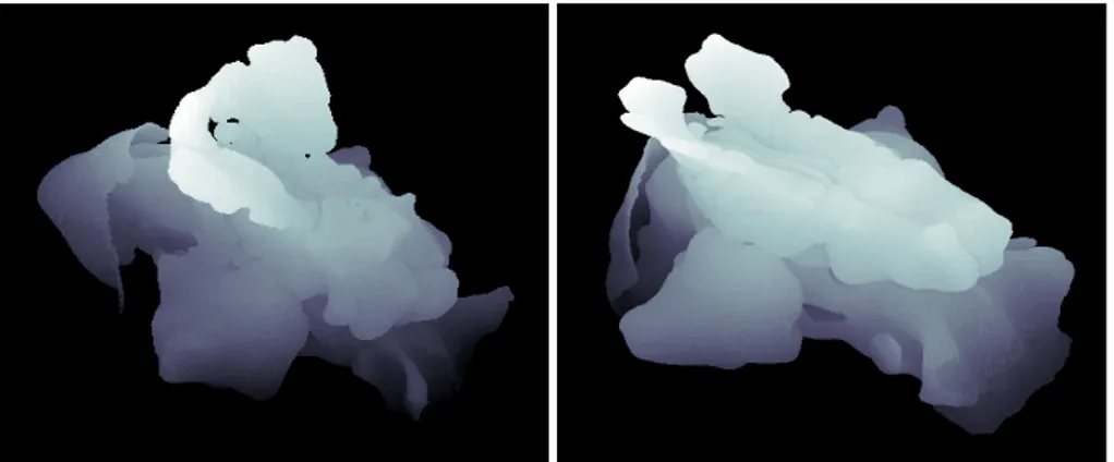
(a) Nasal cavities’ bone structure of ”Cloe” (b) Nasal cavities’ bone structure of ”Flor”

(c) Nasal cavities’ bone structure of ”Gian” (d) Nasal cavities’ bone structure of ”Lian”

Figure 1.1: Manually cleaned nose bone structures.

di Elettronica, Informazione e Bioingegneria at Politecnico di Milano, with the aim of employing Machine Learning techniques in the assess-ment of nasal airflow quality through CFD data to ultimately produce a tool for Computer Aided Diagnosis (CAD).

The aim of this thesis is to facilitate the transition to a phase of the project in which will be used 3D volumes extracted from computerized tomography of real patients instead of the simplified parametric models from the previous phase. As can be seen in Figure 1.2 the morphology of the paranasal sinuses, mostly attached to the upper area of the nasal cavities, is very different from patient to patient.

In order to overcome the burden of medical data preparation, which is really a slow process, we identified a method by which to transfer func-tions that encode small deformafunc-tions from one 3D volume to another. On the CT scans deformed in this way will then be carried out the CFD. First of all, however, it has become fundamental to create a workflow that would allow the autonomous identification of the volumetric areas

(22)

relating to the paranasal sinuses so that they could then be eliminated in a simple way since they are useless for the purposes of fluid dynamics simulations.

(a) Nasal cavities and sinuses bone struc-ture of ”Cloe”

(b) Nasal cavities and sinuses bone struc-ture of ”Flor”

(c) Nasal cavities and sinuses bone struc-ture of ”Gian”

(d) Nasal cavities and sinuses bone struc-ture of ”Lian”

Figure 1.2: Nose bone structures complete of paranasal sinuses.

1.2 Contributions

The openNOSE project involves the intervention of 3 different disci-plines, namely physics, in the context of fluid dynamic computations, medicine, which allows to assign reliable labels to each case from which to start, and finally computer science. The goals of this last field are the creation of a diagnostic tool that produces reliable results easier to understand with reference to the results of fluid dynamic computations and the extraction and manipulation of 3D volumes from CT scans through image processing techniques. It is precisely in this latter area

(23)

that this thesis fits.

The contribution is mainly to overcome the burden of medical data preparation, which is really a slow process. To do this, first of all a method was identified that allowed the match between real-valued functions of two 3D shapes. Thanks to these matches, it is possible to transfer various functions encoding small deformations, obviously under the supervision of a doctor so that they can be as realistic as possible. This allows to obtain a great number of different cases in an easy way and to increase thus the size of the dataset in a short time avoiding to wait for the collection from the hospital.

This goal was achieved using the functional map method, mostly used on very simple volumetric meshes and adapted to the current problem. Furthermore, in order to simplify the load of fluid dynamic computations on such complex volumes, since the paranasal sinuses do not contribute substantially to the airflow inside the nasal cavities, the most immediate choice is to remove them.

Once the 3D volume has been extracted from computed tomography, the elimination of the paranasal sinuses becomes a complex and slow task. This is because in addition to having to correctly identify the areas to be eliminated, manually cutting precisely the aforementioned areas is very difficult due to the their complex morphology which leads them to merge with the walls of the underlying nasal cavities.

A further problem which slows down and makes problematic the elimina-tion of the paranasal sinuses is the fact that they are different in shape and, in some cases, also in number, from subject to subject, Figure 1.2. The contribution of this thesis is therefore to identify these areas au-tomatically and eliminate them easily and precisely. This result was obtained starting from the excellent outcome of the first shape matching method, namely functional map, applied to shapes already without paranasal sinuses. With it has in fact been possible to estimate very reliable point-to-point maps between nasal cavities.

The application domain of this method can be expanded in order to consider as model a shape clean from paranasal sinuses, Figure 1.1, and as target one complete of them, Figure 1.2. Finding a point-wise correspondence between two such shapes means finding only the vertices belonging to the nasal cavities, being them the only parts in common between the two volumes. The remaining unmatched parts are thus necessarily the paranasal sinuses.

The results obtained by using this method are excellent, with an average precision of 0.97, recall of 0.99 and F1-score of 0.98. The method, on average, correctly recognizes 98% of the points and is wrong only on 2% of them considering both the areas of the nasal cavities and those of the paranasal sinuses. Furthermore, since the volumes considered are geometric reconstructions of real noses, the results obtained are even

(24)

less trivial.

1.3 Structure of the Thesis

The contents of this thesis are organized as follows.

First of all in Chapter 2 the OpenNOSE project, of which this work is part, is analyzed in more detail, its long-term goals together with what the project has achieved to date. Then the anatomy of the nose is described, followed by what is a computerized tomography and of the type of objects around which this work revolves i.e 3D volumes extracted from the computerized tomographies themselves.

Chapter 3 introduces the shape matching methods, to which this work refers, together with some techniques for refining the maps extracted with these same methods. In the last part the focus is on another very important medical field to which they have been applied i.e the identification of the Huntington disease.

Chapter 4 contains first a detailed description of how has been ap-proached the problem of extracting a map that allows to put in cor-respondence real-valued functions of two volumes without paranasal sinuses. Then an analysis of the expansion of the application domain of this first method in order to autonomously identify the paranasal sinuses in a target volume starting from a model one clean of them. In Chapter 5 the experimental results of both methods described in Chapter 4 are analyzed, also focusing on how these results were ex-tracted, which is not trivial given the lack of a ground truth.

Finally, Chapter 6 contains the conclusions of the work done and further perspective for future work.

(25)

Chapter 2

OpenNOSE Project

In this chapter I will explain the context to which this work belongs, the long term goals and were the openNOSE project got to today. Furthermore I will show some Computerized Tomography Scan paired to core functions and characteristics of the human upper airways.

2.1 Long term goals

The project called OpenNOSE, conducted in collaboration with the group of otolaryngology of the A. O. San Paolo di Milano and with Universit`a degli studi di Milano, has the aim of providing doctors and surgeons with an effective, open-source and patient-specific support in order to decrease time, costs and side effects on patients in the field of diagnostics and interventions.

The continuous increase in the performance of the computers has made it possible to considerably reduce the calculation times, until in some cases a numerical simulation can be considered more convenient than an experimental one.

Starting from this consideration the goal is to develop a procedure that allows to diagnose in an autonomous way not only the presence of a possible pathology but also, if it occurs, from which pathology the patient is affected.

For this project, the first discipline that becomes indispensable is, of course, medicine, as it is precisely through doctors and hospitals that the dataset, made up of computerized tomography scans of real and voluntary patients, can be expanded.

Doctors also provide an excellent basis from which to start the identifi-cation work as they are able to diagnose the disease and provide thus the fundamental labels for training and validation of the autonomous classification process that will be carried out.

The second fundamental element is physics, the project has in fact the objective of classifying nasal pathologies from data extracted from

(26)

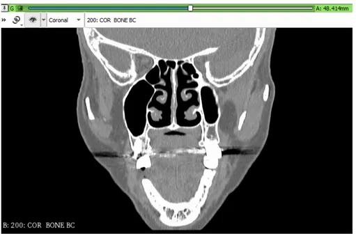
Figure 2.1: Sagittal view of a computerized tomography scan

fluid dynamic simulations RANS (Reynolds-averaged Navier-Stokes) and LES (Large Eddy Simulation) performed both in steady inspiration and exhalation, with different boundary conditions and with the use of numerical schemes of the first and second order.

To finish the computer science, area in which this thesis work is located, necessary for the study of data extracted through CFD (computational fluid-dynamics) from the analysis of the fluid current in the geometry of the nasal cavities.

The results of the simulations come used as tests and validation sets to build a classifier that is able to separate healthy patients from sick ones and in addition to assign each patient of the sick group to a specific subgroup related to the disease that affects him.

In addition, it has the task of preparing the field for CFD by recon-structing a three-dimensional geometry of the nasal cavities, as the one in Figure 2.8 starting from the patient’s computed tomography (CT) images, Figures: [2.1(sagittal view), 2.2(coronal view), 2.3(axial view)]. It is essential to guarantee the quality of the mesh, a fundamental aspect to ensure the convergence of the computational fluid-dynamics (CFD) to an exact solution.

2.2 OpenNOSE Project to Date

The first stage of the openNOSE project involved the use of simplified parametric models as the collection of data from real noses would have been expensive for an introductory study.

(27)

Figure 2.2: Coronal view of a computerized tomography scan

It involved thus the development of a simplified parametric model that represented the nasal cavities well enough, both in terms of topology and characteristics of the air flow.

Given the need for a large and varied dataset starting from a first basic shape, by modifying some control parameters that introduced structural changes, a good number of different models have been obtained. All the changes made to the noses, even if synthetic, have been supervised by a doctor of the team of collaborators of the Ospedale San Paolo di Milano in order to introduce both pathological and non-pathological changes within the structure of the synthetic noses.

A fluid dynamic simulation of the RANS (Reynolds averaged Navier-Stokes) type was therefore carried out on each of these models, obtaining a dataset suitable for experimentation on the management of this type of high-dimensional information.

Having obtained these data extracted from the CFD, the objective is to predict, for each nose of the dataset constructed as described above, whether it belongs to the group of healthy patients or to the group of sick patients and, in the latter case, to which of the various pathologies through the value of the relative parameter.

Given the difficulty of defining reliable labels for the models created, it was decided, for this first step, to work in a context of regression rather than classification.

The first thing to do, however, was to limit the size of the data obtained, first of all some components of the simulations deemed interesting were

(28)

Figure 2.3: Axial or transverse view of a computerized tomography scan

extracted with an expert approach, such as the field values on sections of the model in correspondence of some landmarks, to then calculate, with a feature engineering approach, features that could represent, in a compact way, the most relevant information from the reduced data. Various feature selection techniques were then applied to these features with the aim of identifying and extracting only those most useful for prediction.

Finally, for each pathological modification, a regression model with the best selected features was trained, studying the quality of the results as the number and type of these features varied.

After this first phase in which simplified parametric models have been taken into consideration, the goal of the openNOSE project is to move on to the analysis of real subjects.

Unlike in the case of synthetic noses, it is very difficult to have a large number of cases, precisely because they are extracted from computerized tomography scans of real patients. In addition to this another problem is that of cataloguing the obtained cases assigning labels as healthy or, if not, which kind of pathology the patient is affected by. Furthermore, extracting data from real cases involves some technical problems from the point of view of acquiring the 3D shape starting from computerized tomography.

This is because, starting from a computerized tomography, a much more precise nose model is obtained, but also much more complex than the parametric model referred to in the first phase of the work.

(29)

Figure 2.4: Sagittal view of anatomical features of the nose.

model from the model currently being analyzed is the presence of the paranasal sinuses, complex and different in each individual in shape and size, as described in Section 2.3, and also useless for what regards the CFD.

In addition to the improvement of the 3d model, which goes from being a simple parametric model to a model extracted from a real nose, the goal is also to improve the CFD technique by switching to a LES type, a middle ground between RANS modeling (Reynolds averaged navier-stokes) faster but more approximate, used previously, and a DNS (direct numerical simulation).

2.3 Nasal Cavities

It is of fundamental importance, for the reading ahead, to become famil-iar with some basic concepts about the nose anatomy and physiology [4, 5, 6] and to get a grasp on the terminology and on the kind of objects that will be consistently used throughout the course of this document. First thing to know is the classical nomenclature of the axes of the human body in medicine.

There are three principal planes, as can be seen in Figure 2.5: The sagittal plane or median plane (longitudinal antero-posterior) is a plane parallel to the sagittal suture (from which it takes its name) and divides the body into right and left part, the coronal or frontal (vertical) plane divides the body into dorsal and ventral part (anterior and posterior), and finally the transverse or axial plane (lateral, horizontal) divides the body into a cranial and caudal part (head and tail).

(30)

2.3.1 Anatomy

From an anatomical point of view, attention must be paid to the main nasal cavities’ features, which are illustrated in Figure 2.4 and Figure 2.6.

The nasal cavity is located between the oral cavity and the skull base, precisely above the hard palate.

It is divided into two sections, also known as fossae, by the septum, which is made of cartilaginous tissue near the nares and becomes bony in the inner portion near the nasal choanae.

Ethmoid bone, vomer bone and maxilla bone contribute to the region of the septum made of osseous tissue.

The septum ends at the back of the nose, where the two nasal cavities join into one when entering the nasopharynx that connects the nasal cavities to the oropharynx.

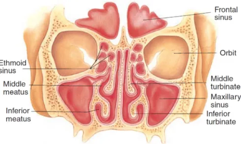
Observing the nasal cavities that form a coronal cut, Figure 2.6 it can be seen how the two passages, formed on the left and right sides of the septum, are limited by some curly bone structures known as turbinates. These formations are of primary importance for air conditioning since they are covered in soft tissue and mucosa, and their peculiar shape strongly increases the amount of mucosal surface inside the nose, helping heat transmission.

Figure 2.5: Main anatomical planes

Usually there are three turbinates per nasal cav-ity, inferior, middle and su-perior, with variable pres-ence of a fourth one, called supreme turbinate, from case to case.

Below each turbinate runs a corresponding meatus, which consists of a natu-ral canal left open in the cavity by the protruding bone.

The inferior tubinate is the largest of the three and plays a crucial role in

air-flow warming and humidifycation with a blood vessels pillow, along its length, which acts as a radiator.

It spans the entire length of the lateral nasal wall, right above the nasal floor, and acts as a sink, with the meatus underneat, for the nasolacrimal duct.

(31)

Figure 2.6: Coronal view of the anatomical features of the nose.

The middle turbinate is located just above the inferior turbinate, it connects with the lateral nasal wall and ends below the skull base.

In this case the frontal sinus, maxillary sinus and anterior ethmoid sinus cells drain into the middle meatus beneath.

Finally the superior turbinate is the smaller of the set and attaches between the nasal wall and the base of the skull.

The space between nasal septum and superior turbinate, which is called sphenoethmoid recess, is a sink for the sphenoid sinus and the posterior ethmoid sinus cells.

At the end there is the nasal valve, a structure formed by the superpo-sition of upper and lower lateral cartilage, the septum and the lower tubinate, located immediately after the nostrils, at the entrance of the nostrils.

This area is the one which poses the maximum resistance to airflow. Finally the paranasal cavities, one of the most variable parts in the human nose, these cavities are connected to the nasal ones, treated so far, and they have the function of modifying the characteristics of the inspired air, of lightening the frontal massif and of helping the resonance during the emission of the sounds; they are sinuses carved into the bones from which they take their name.

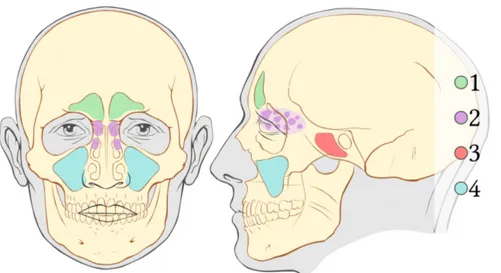
There are four types of paranasal sinuses, as can be seen in Figure 2.7 approximately symmetrical with respect to the sagittal plane, which take their name, as mentioned above, from the bones within which each sinus lies.

Starting from the top, the frontal sinuses are presented first, positioned above the orbits in the frontal bone, connected to the anterior part

(32)

Figure 2.7: Paranasal sinuses from a coronal and sagittal view: 1: Frontal Sinuses. 2: Sphenoid Sinuses. 3: Ethmoid Sinuses. 4: Maxillary Sinuses.

of the middle nasal meatus through the frontonasal duct and which constitute the hard part of the forehead.

Going down, in the space between the nasal septum and the superior turbinate (sphenoethmoid recess), there are the sphenoid sinuses posi-tioned in the sphenoid bone, quite smaller and more numerous than the frontal sinuses, they can vary from individual to individual not only in size but also in the shape, and because of their lateral position with respect to the septum they are rarely symmetrical.

Continuing downwards, between the sphenoethmoid recess and the middle meatus, the ethmoidal sinuses, or ethmoidal air cells, appear positioned in the ethmoid bone and they too, like the sphenoid sinuses, can vary in size and even number form.

They are divided into anterior, very close to the sphenoid sinuses, and posterior, closer to the maxillary ones, from the basal lamella, one of the bone divisions of the ethmoid bone contained in the ethmoidal labyrinth. Finally, the largest, maxillary sinuses, positioned under the orbits in the maxillary bone, are pyramid-shaped and flow into the middle meatus through the osteomeatal complex.

On top of what currently stated, additional complications are added by the cycles of congestion and decongestion, which have variable peri-odicity based on the current season or even the time of the day. These cycles are responsible for temporary modifications of airflow qual-ity with the narrowing of pathways or the occlusion of ducts linking sinuses and meatuses.

(33)

Figure 2.8: A blender view of a volume complete of paranasal sinuses

2.3.2 Compuerized Tomography Scans

The objects with which I have worked and on which this work is centered are 3D shapes modeled as two-dimensional Riemannian manifolds M (possibly with boundary) equipped with an intrinsic distance function

dM and the standard area element dµ.

This 3D shapes are extracted from computerized tomography scans (CT-scans), this scans combine a series of X-ray images taken from different angles around the body, in this case only the face area, and use computer processing to create cross-sectional images (slices) of the bones, blood vessels and soft tissues.

The most interesting parts of this CT-scans for this work are the cross-sectional images which allow to reconstruct the internal bone structure of the patient’s noses Figures: [2.1(sagittal view), 2.2(coronal view), 2.3(axial view)], this is because, as stated before in Section 2.1, the fluid dynamic simulation of the air flow of the upper respiratory tract is carried out through the empty cavities of the 3D shape.

Once the bone scan has been isolated, the CT scan can be transformed into a 3D shape using, in this case, 3Dslicer software, an open-source medical imaging program.

I now have a .stl file which describes only the surface geometry of the three-dimensional object, namely the internal bone structure of the nose without any representation of color, texture or other common model attributes, as can be seen in Figure 2.8.

A .stl (Standard Triangulation Language) file describes a raw, unstruc-tured triangulated surface by the unit normal and vertices of the triangles

(34)

Figure 2.9: A blender view of a coronal slice of a volume complete of paranasal sinuses

using a three-dimensional Cartesian coordinate system, it contains no scale information and the units are arbitrary.

As can be seen from Figure 2.9 all the anatomical features of the upper respiratory tract, described in section 2, are easily identifiable even in the sections of the triangulated surface.

The manifold obtained in this way, however, still presents paranasal sinuses as the one in Figure 2.8 which, as specified in Section 2.2, are not useful for the purpose of predicting pathologies through fluid dynamics simulation, will therefore be one of the main objectives of this thesis work to remove them in an automatic fashion.

(35)

Chapter 3

Shape matching

Shape matching is the problem to find a point-to-point correspondence between shapes. These shapes are commonly represented as polygonal meshes or point clouds. The goal of a shape matching algorithm is to find a map between the two set points that define the shapes.

Functional maps is a solution for the shape matching that solves for the correspondence between points through the alignment of the functional spaces defined on them. In this chapter I will introduce the shape matching methods that underlie this thesis work. First of all I will show the functional maps algorithm by Maks Ovsjanikov et al. [7] today considered as a specific sphere of solution of the shape matching. Within this area, due to the positive aspects of the functional approach, such as invariance at the number of points, invariance with non-rigid isometric variations and efficiency, in the last ten years different methods have been proposed each with the aim or to refine the quality of matching [8] or to extend the application domain of the method [9, 10].

3.1 Functional Maps

In a rigid transformation the space of deformations is limited to isome-tries, i.e functions between metric spaces that preserve distances. This kind of transformation can be represented in a compact way such as rotation, translation, rescaling and reflection. Conversely, non-rigid shape matching remains difficult even when the space of deformations is limited to approximate isometries. This is because they are most frequently represented as correspondence of points or regions on the two shapes.

The more detailed the analyzed shape is, the higher the number of points will be. It is so infeasible to optimize directly over point-to-point correspondence. For this reason most shape matching methods, in the non-rigid case, such as [11, 12, 13, 14, 15, 16, 17, 18], aim to obtain a sparse set of point-to-point correspondences and then extend it to

(36)

more dense mappings. Furthermore, being these sparse correspondences inherently discrete, some ways to enforce global consistency include the preservation, between pairs or sets of points, of geodesic distances [11, 12, 18], a combination of multiple geometric and topological tests [19, 14], various spectral quantities [20, 21, 22, 15], or embedding shapes into canonical domains [13] based on landmark correspondences. Another set of techniques aims to establish shape part or segment cor-respondences rather than reliable point-to-point matches, e.g. [23, 24, 25, 26, 27]. Such techniques either pre-segment the shape and try to establish part correspondences, or phrase the segmentation and corre-spondence in a joint optimization framework [25, 26, 28] which generally avoids the need to establish reliable pointwise correspondences.

The common characteristic of all this non-rigid shape matching meth-ods is that they lead to difficult, non-convex, non-linear optimization problems.

A novel approach for inference and manipulation of maps between shapes that overcame this issue trying to resolve it in a fundamentally different way is functional maps.

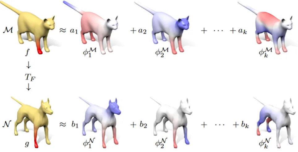
Instead of putting directly in correspondence points on the two shapes, it consists in considering matchings between functions defined on the shapes, see Figure 3.1(a). Basically, using a small number of Laplace-Beltrami bases for the functions spaces of the two shapes, the map can be well-approximated with a relatively small matrix, as the one in Figure 3.1(b), that from here on will be identified as C.

(a) Source to Target map

10 20 30 40 50 5 10 15 20 25 30 35 40 45 50 0 0.1 0.2 0.3 0.4 0.5 0.6 0.7 0.8 0.9 1

(b) Matrix C encoding the map

Figure 3.1: Functional maps result on Tosca dataset (a) with relative matrix C (b).

3.1.1 Laplace-Beltrami Operator

A fundamental choice is that of the bases functions φM_i on shape M and φN_j on shape N. I need compactness, because the simplest elements

(37)

of a shape must be represented with as few basis functions as possible, and stability, namely the space of functions spanned by the linear com-bination of the basis functions must be stable with reference to small deformations.

Respecting these two properties allows to represent the transformation TF using only a relatively small subset of basis functions and to therefore retrieve a finite matrix C that represents it compactly.

In differential geometry, the Laplace-Beltrami operator is a self-adjoint differential operator that generalizes the Laplace operator to functions defined on Riemannian varieties. A Riemannian variety is a differen-tiable variety (curve or surface) on which the notions of distance, length, geodesic, area (or volume) and curvature are defined. Variety is a topo-logical space which is locally similar to a well-known topotopo-logical space such as the Euclidean one but which globally can have different geomet-ric properties such as being curved. The Laplace-Beltrami operator is thus the extension to non-Euclidean cases of the standard Laplacian and can be discretized. The eigenfunctions of this operator are the par-allel with the Fourier bases and are ordered according to their absolute value which is an analog of the Fourier frequencies. So the choice of eigenfunctions of the Laplace-Beltrami operator becomes natural since they are ordered from the lowest frequency to the higher ones, meaning that they provide an inbred multi-scale way to approximate functions. Taking a finite set associated with minor eigenvalues is equivalent to a low pass representation of functional spaces. So in this representa-tion the funcrepresenta-tional map is represented by the transformarepresenta-tion matrix of the Fourier coefficients and is compact and easy to optimize. This optimization is based on the alignment of a set of functions that can be calculated on both shapes and which is known to correspond to each other.

So the first thing necessary to exploit this method is to compute a set of descriptors for each point on both shapes, M and N, and then starting from them create some function preservation constraints. I will not focus much on this point for now because it is highly dependent to the kind of shapes to be matched, it will be better described in Chapter 4. A general solution proposed for this is to use landmarks, corresponding regions or descriptors as the Wave Kernel Signature (WKS) [29] and Heat Kernel Signature (HKS) [30].

The wave kernel signature exploits the Schr¨odinger wave equation in order to characterize a point x ∈ X by the average probabilities of quantum particles of different energy levels to be mesured in x. Since energies of particles correspond to frequencies, in this approach informa-tion from all frequencies is captured while at the same time influences from different frequencies are clearly separated.

In a similar way Heat Kernel Signature exploits instead the heat

(38)

sion equation in order to characterize a point x ∈ X by the amount of heath measured in x at certain times t > 0.

Let’s now consider two manifolds, M and N, and T : M → N a bijective mapping between them.

Considering spaces of only real-value functions F (·, R) on both shapes means that given a scalar function f : M → R I can obtain by composi-tion a scalar funccomposi-tion g : N → R, knowing that g = f ◦ T−1.

This induced transformation can be denoted as TF : F (M, R) → F (N, R).

Every function f : M → R can be represented as a linear combination of basis functions φM_i as f =P

iaiφMi .

In the same way I can also apply to N a set of basis functions φN_j , doing so I can consider TF(φM_i ) =P

jcijφNj for some cij and TF(f ) = X i ai X j cijφN_j =X i X j aicijφNj (3.1)

Therefore, considering f as a vector of coefficients a = (a1, a2, . . . , ai, . . . ) and g = TF(f ) as another vector of coefficients b = (b1, b2, . . . , bi, . . . ) then equation (3.1) simply becomes bj =P

iaicij, where cij is completely independent from the chosen function and is determined only by the bases and the map T as can be seen in Figure 3.2.

Figure 3.2: Basis functions applied to source shape M and target shape N.

3.1.2 Functional Matrix C

Since as stated above I have i basis functions φM_i on shape M and j basis functions φN_j on shape N, the matrix C that represents the

(39)

mapping TF will be of dimension kM × kN.

Being C dependent only from the map TF and from the basis func-tions means that considering as before f as a vector of coefficients a = (a1, a2, . . . , ai, . . . ) I obtain that TF(a) = Ca.

In addition to this, if the shapes M and N are isometric and T is an

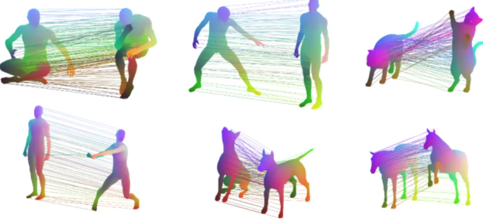
Figure 3.3: Some functional maps results

isometry, matrix Cij can be non-zero only if φM_i and φN_j correspond to the same eigenvalue. In particular, if all eigenvalues are non-repeating, matrix C will be diagonal.

As can be seen in figure 3.3 in the considered cases the shapes are non-rigidly deformed so T is only approximately an isometry, this makes the matrix C still close to diagonal, or funnel shaped, as can be seen in figure 3.1(b).

It is a must to underline the fact that the matrix C stops being diagonal with just small non-isometric deformations, and this can be noticed particularly starting from the high frequencies eigenfunctions.

(40)

Algorithm 1 Functional Maps Inference for Matching

1 Compute a set of descriptors for each point on M and N, and create function preservation constraints.

2 If landmark correspondences or part decomposition constraints are known, compute the function preservation constraints using those. 3 Include operator commutativity constraints for relevant linear operators

on M and N (e.g. Laplace-Beltrami or symmetry).

4 Incorporate the constraints into a linear system and solve it in the least squares sense to compute the optimal C.

5 Refine the initial solution C using one of the iterative methods proposed below.

6 If point correspondences are required, obtain them using the equation (3.2).

3.2 Functional maps refinements

The next step after the extraction of the matrix C is to proceed to a post-processing iterative refining. I can take into consideration two different methods: Iterative Closest Point (ICP) or iterative spectral upsampling named ZoomOut as the first proposed and the most recent respectively.

3.2.1 Iterative Closest Point map refinement

The first proposed method is identical to the standard Iterative Closest Point (ICP) algorithm of Besl and McKay [31] with the only difference that in this case it is applied in the spectral embedding rather than on the simple Euclidean space.

Given ΦM the matrix of the Laplace-Beltrami eigenfunctions of M and ΦN the matrix of the Laplace-Beltrami eigenfunctions of N, where each column corresponds to a point and each row to an eigenfunction, I can obtain the image of the delta function centered in each point of M simply as CΦM.

Let’s now suppose to have a starting map C0 that I believe comes from a point-to-point map T, this means that each column C0ΦM coincides with some column of ΦN.

If I now consider ΦM as a point cloud with dimensionality equal to the number of basis functions of M and ΦN as another point cloud with dimensionality equal to the number of basis functions of N, this means that C0, of dimensions i × j, must align ΦM and ΦN.

This means that ICP iteratively modifies C trying to align more and more CΦM to ΦN.

(41)

3.2.2 ZoomOut map refinement

Another way to post-process the resulting matrix C is through iterative spectral up-sampling.

Early spectral methods for shape correspondence were based on directly

Figure 3.4: Functional maps upsampling result starting from a 2 × 2 matrix. (Figure adapted from [8].)

optimizing pointwise maps between spectral shape embeddings based on either adjacency or Laplacian matrices of graphs and triangle meshes [15, 20, 21, 32, 33, 34].

Differently from the method described above this time I can use as input either a small matrix C0 or a point-to-point map T : M → N both of which may be affected by noise.

While with Iterative Closest Point the starting matrix C0 has the same dimensions as the resulting matrix C obtained after the post-processing, with ZoomOut [8] given an input functional maps matrix C0 of di-mensions kM × kN, where kM < i are the first kM columns of the Laplace-Beltrami eigenfunctions matrix ΦM_i and kN < j are the first kN columns of the Laplace-Beltrami eigenfunctions matrix ΦNj , the goal is to extend it to a new functional maps matrix C1 of dimensions (kM + 1) × (kN + 1) without any additional information.

This is accomplished by computing a point to point map T via a nearest-neighbour query in a kM-dimensional space as follows:

T (p) = arg min q k C(ΦN_k N(q)) >_{− (Φ}M kM(p)) > _k 2, ∀p ∈ M (3.2) Where ΦM_k M(p) denotes the p

th _{column of the matrix of the} eighenfunc-tions of Laplace-Beltrami operator. Once obtained the point-to-point map it can be encoded into a matrix Π so that Π(i, j) = 1 if T (i) = j

(42)

and 0 otherwise. Now the starting functional maps matrix C0 can be extended in this way:

C1 = (ΦMkM+1)

>_A

MΠΦNkN+1 (3.3)

Where AM is a diagonal matrix of the lumped area elements. I now

Figure 3.5: Functional maps after applying ZoomOut example results. (Figure adapted from [8].)

iterate this two steps in order to obtain progressively larger functional maps C0, C1, C2, . . . , Cn until some sufficiently large n. In Figure 3.5 can be seen from left to right in first column upper row the source shapes, first column bottom row the target shapes. From second to last column starting with a noisy functional maps represented by a matrix C of size 5 × 5 I up-sample it progressively and show the corresponding point-to-point map at each iteration via color transfer. Note that the final matrix can’t possibly be larger than i × j where i is the number of basis functions φM_i on shape M and j the number of basis functions φN_j on shape N.

(43)

Algorithm 2 ZoomOut

Input: C0 size kM× kN, n × m (desired final size of C ), stepSZ = steps size, ΦM_i , ΦN_j , AM

Output: Cn size m × n

Data: Manifold M, Manifold N

/* External loop, iterates until reaching the desired size of C */

1 while kM < m & kN < n do

/* For each point p ∈ M finds the corresponding point T (p) ∈ N */

2 for p=1:size(M) do 3 T (p) = arg min q k C(ΦN kN(q)) >_{− (Φ}M kM(p)) > _k 2

/* Encode the point-to-point map into matrix Π */

4 if T (p) = q then

5 Π(p, q) = 1

6 else

7 Π(p, q) = 0

/* Extend the matrix C from size kM × kn to size kM + stepSZ × kN+

stepSZ */

8 C = (ΦM_k

M+stepSZ)

>_A

MΠΦNkN+stepSZ

3.3 Matching deformable objects in clutter

On the one hand, shape matching concerns the problem of determining a dense correspondence between two given objects. On the other hand, object recognition consists in locating, and at the same time putting into correspondence a template model within a given scene which contains the object of interest. A particularly challenging instance of this problem arises when the object to be sought is allowed to deform in a non-rigid fashion. Despite the conceptual similarities, however, 3D shape match-ing and recognition have been tackled separately and under different assumptions. Deformable matching techniques assume the absence of additional objects (clutter); conversely, object-in-clutter methods rely on the scene to contain a rigidly transformed instance of the model. The problem of 3D object detection in cluttered scenes has been tackled for several years by the computer vision community as recently studied in [35].

Some good approaches couple the detection of local rotation-invariant surface features [36] together with some geometric consistency criterion to drive the matching. Candidate matches are first selected according to the similarity of the local features and then pruned by excluding geometrically inconsistent candidates.

Some popularly used consistency criteria include four-points congruent sets [37] and minimum pairwise Euclidean distortion [38].

(44)

Machine learning techniques have also been proposed to learn optimal local features in the presence of clutter [39], or to learn the consistency function itself [40, 41]. Despite their excellent performance in several computer vision tasks, however, all these methods fail completely when the objects undergo non-rigid deformations.

The method exploited and analyzed here is the one from L. Cosmo et al. [10]. The matching pipeline is the same proposed in [7] by Maks Ovsjanikov et al. described above. The main idea is still to identify cor-respondences between shapes by a linear operator T : M → N , mapping functions on M to functions on N. This can be seen as a generalization of classical point-to-point matching, as the latter constitutes a special case where one maps delta functions to delta functions.

Figure 3.6: Functional correspondences at increasing amounts of clutter.

3.3.1 Functional matrix C for objects in clutter

Being T a linear operator it admits a matrix representation C which coefficients cij are computed as in function (3.1). A particularly con-venient choice for the basis functions is, again, given by the Laplacian eigenfunctions of the two shapes as proposed above and exploited in [7]. By analogy with Fourier analysis, this choice allows to truncate the series (3.1) after the first k coefficients as a low-pass approximation of the original map, giving rise to a k × k matrix C encoding the functional correspondence. Furthermore, if the functional maps T is built on top of a near-isometry, one obtains cij = hT φMi , φNj iN ≈ ±δij since near-isometric shapes have corresponding eigenfunctions (up to sign). This results in matrix C being diagonally dominant, as stated above, since cij ≈ 0 if i 6= j.

Let us now assume to be given a full shape M and a partial shape N that is approximately isometric to some (unknown) sub-region M0 ⊂ M . Recently, Rodol‘a et al. [9] showed that for each “partial” eigenfunction φN_j of shape N there exists a corresponding “full” eigenfunction φM_i of shape M for some i ≥ j, such that cij = hT φM_i , φN_j iN ≈ ±1, and zero

(45)

otherwise.

Note that differently from the previous case (full-to-full), where the approximate equality holds for i = j, here the inequality i ≥ j induces a slanted-diagonal structure on matrix C. In particular, the authors showed that the angle of the diagonal can be directly and conveniently estimated from the area ratio of the two surfaces. The precomputed angle is then used as a prior on C to drive the matching process [9]. While, as already said, in the full-to-full case I had correspondence for i = j and in the part-to-full case for i ≥ j, here the correspondence among indices cannot be reliably predicted. The diagonal slant of C, which identifies the pairs (i,j) for which cij = hT φM_i , φN_j i_N 6= 0, is now an unknown that I need to optimize for. In particular, I expect cij 6= 0 only for a sparse set of indices, i.e., matrix C will have empty rows and columns, see Figure 3.6 where every matrix on the bottom row encodes the transformation from the model M to the various scenes (N1, N2, N3, N4).

From left to right I start with a clutter-free scene that is partial with reference to the model M and increase the clutter amount with each scene. It can be observed that the dominant slope of Ci, denoted by Θ, varies with clutter, moving from the lower to the upper-triangular part of the matrix. Furthermore the rank of Ci decreases as more and more clutter is introduced, fact denoted by empty rows and columns in Ci and by the sparsity of the diagonal in C_i>Ci.

It is worth mentioning that the slant of C directly encodes the amount of overlap between model and scene [9], hence providing an important prior for the correspondence. Litany et al. [42] recently showed (for non-rigid puzzles) that the slant can be simply estimated as the area ratio of the two objects, in our case area(M )_{area(N )}, where M is the model and N is the scene. However, this property fails to hold when the amount of clutter in the scene is significant.

3.3.2 Functional objects in clutter

Let ΦM_i ∈ R|M |×i and ΦN_j ∈ R|N |×j be two matrices containing as columns the first i and j Laplacian eigenfunctions of M and N re-spectively, and let matrices F ∈ R|M |×d and G ∈ R|N |×d contain dense d-dimensional descriptor fields on model and scene.

The aim is to solve, again as in the functional maps case, for the map C between M and N. In addition to this the minimization problem takes into consideration also the angle Θ ∈ R encoding the diagonal slope of C, and the (soft) segmentation functions u : M → [0, 1] and v : N → [0, 1] identifying the corresponding regions on model and scene.

This is because differently from the previous case (full-to-full), where

(46)

Figure 3.7: Some results of functional objects-in-clutter pipeline. (Figure adapted from [10].)

the approximate equality holds for i = j, here the inequality i ≥ j induces a slanted-diagonal structure on matrix C that has to be encoded into the minimization problem. The soft segmentation functions u and v are added in order to identify the model shape into the target one. I therefore consider the unconstrained problem:

min

C,Θ,u,v k CA(η(u)) − B(η(v)) k2,1 + k CΦM >_i η(u) − ΦN >_j η(v) k2₂

+ ρcorr(C, Θ) + ρpart(u, v)

(3.4)

The first part of the equation, (3.4), is basically the same as the one of the basic functional maps problem [7]. Assuming i = j = k, here A(η(u)), B(η(v)) ∈ Rk×d contain the spectral coefficients of F and G masked by the respective segmentation functions u and v, i.e., for each column of A(η(u)) I write ai = ΦM >i (η(u) ◦ fi), and for each column of B(η(v)) bj = ΦN >j (η(v) ◦ fj).

η(t) = 1₂(tanh (2t − 1) + 1) is a saturation function applied in order to keep the range of u and v within [0, 1] as done in [9].

As descriptor fields, I can use as in [7] Wave Kernel Signature [29] or Heat Kernel Signature [30], in addition to indicator functions supported at some landmark matches.

The L2,1 norm allows to handle possible mismatches arising from the Quadratic assignment problem.

The L2 summand in the data term simply asks for the functional maps to correctly transfer the segmentation functions.

The last term is composed of two regularization terms: the first one for the matrix C and the second one for u and v. The first regularization term, the one relating to the functional maps matrix C, is:

ρcorr(C, Θ) = µ1 X i6=j (C>C)2_ij+ µ2 X i | C>C |ij +µ3 k C ◦ W (Θ) k2F (3.5)

(47)

Algorithm 3 Functional Objects-in-Clutter Input: F ∈ R|M |×d, G ∈ R|N |×d← N.lm

Output: C, Θ ∈ R, u : M → [0, 1],v : N → [0, 1]. Data: Manifold M, Manifold N, funtion f

1 Extract ΦM_k ∈ R|M |×k and ΦN_k ∈ R|N |×k // The first k Laplacian eigenfunctions of M and N

2 η(t) = 1₂(tanh (2t − 1) + 1) // Saturation function used to maintain the range of u and v within [0,1]

/* Build A(η(u)) and B(η(v)) containing the spectral coefficients of F and G masked by the respective segmentation function u and v. */

3 for i=1:k do 4 ai= ΦM >_i (η(u) ◦ fi) 5 A(η(u))(:, i) = a_i 6 for j=1:k do 7 bj = ΦN >_j (η(v) ◦ fj) 8 B(η(v))(:, j) = bj

/* Regularization term for matrix C and for its diagonal Θ. */

9 ρcorr(C, Θ) = µ1P_i6=j(C>C)2_ij + µ2P_i | C>C |ij +µ3 k C ◦ W (Θ) k2_F

/* Regularizaion term for the segmentation functions u and v. */

10 ρ_part(u, v) = µ₄(R_M k ∇_Mη(u) k dx +R_N k ∇_Nη(v) k dx) +µ5(R_Mη(u)dx −R_Nη(v)dx)2

−µ₆(R

Mη(u)dx + R

Nη(v)dx)

/* Unconstrained minimization problem over matrix C, its diagonal angle Θ and the two segmentation functions u and v. */

11 min

C,Θ,u,vk CA(η(u)) − B(η(v)) k2,1 + k CΦM >_i η(u) − ΦN >_j η(v) k2₂ +ρcorr(C, Θ) + ρpart(u, v)

with a sparse diagonal, inducing so empty rows and columns in C as can be seen in figure 3.6 hence reinforcing its slanted diagonal structure. In addition, the two terms promote area preservation, as for area-preserving functional maps it has been shown that C>C = I [7, 9]. Note however that this identity, as already stated before, only holds in the full-to-full case: Since our C has empty rows and columns, I only require the identity to hold approximately at a sparse set of elements. This corresponds to requiring the matched parts to have equal area. Finally,W (Θ) is a diagonal mask parametrized on the slope Θ, requiring a similar structure on C (here ◦ is an element-wise product).

The second regularization term, the one relating to the segmentation

(48)

(a) Mask η(u) on M and η(v) on N.

(b) Masked functional correspondence.

Figure 3.8: Functional objects in clutter mask and functional correspondence.

functions u and v, is:

ρpart(u, v) = µ4( Z M k ∇_Mη(u) k dx + Z N k ∇_Nη(v) k dx) + µ5( Z M η(u)dx − Z N η(v)dx)2 − µ₆( Z M η(u)dx + Z N η(v)dx) (3.6)

The µ4-terms, in the first line of the equation, encodes the boundary length of the segmentation functions on the respective shapes. Here ∇N denotes the intrinsic gradient operator on shape M and similarly ∇N for scene N. Following the spirit of the Mumford-Shah functional

(49)

[43], penalizing boundary length has the effect of producing contiguous regions, as expected in our setting.

The µ5-term requires the two parts to have same area, while the µ6-term controls the size of the parts (a large weight will promote large areas and viceversa).

Note that this term is necessary in order to avoid the trivial solution u = 0, v = 0, C = 0.

3.4 Shape matching methods in medical domain

An extension of Functional Maps to the medical domain is the work from S. Melzi et al. [44]. They evaluated a method for the characterization of brain abnormalities in the context of mental health research. In particular, they propose a brain classification study on a dataset of patients affected by bipolar disorder and healthy controls.

The functional representation of brain shapes, or their subparts, enables to improve the detection of morphological abnormalities associated with the analyzed disease.

In this case the focus is on the putamen region, which is a deep

Figure 3.9: A mapping of real-valued functions between pial surfaces.

gray matter brain structure, part of the basal ganglia, a functional

(50)

and anatomical heterogeneous region which is thought to be affected, particularly in shape, by bipolar disorder.

The proposed method is based on the spectral shape paradigm that is used for generic geometric processing but still few exploited in the medical context.

The key aspect of the Functional maps framework [7], as described above, is that it moves the estimation of correspondences from the shape space to the functional space enhancing the potential of spectral analysis. The obtained results for bipolar disorder detection on the putamen re-gions are promising in comparison with other spectral-based approaches. This work proposes a spectral framework, namely Brain Transfer, to transfer functions between different shapes, in order to explore the shape and functional variability of retinotopy.

Conversely, to obtain and analyze this representation propose the use of the Functional maps framework [7]. This construction is founded on the Laplace Beltrami Operator (LBO) eigendecomposition and involves the diffusion of spectral descriptors and their desired properties.

(51)

Chapter 4

Shape matching and

OpenNOSE

In this chapter I will show how I applied the shape matching techniques previously explained in Chapter 3 to the problem of the OpenNOSE project. First I will focus on the matching of real-valued functions between two ideal noses, that is, already cleaned from the paranasal sinuses.

Finally I will show how I dealt with the problem of automatic paranasal sinuses removal. The first two steps, the choice of basis functions and the landmark selection, are common to both methods so they have been summarized separately.

(a) Model shape M (b) Target shape N

(52)

Figure 4.2: Basis functions φM

i applied on model shape M

4.1 Problem Formulation

First I extract the volumetric meshes representing the complete nasal cavities from the CT scans and I clean them manually from the paranasal sinuses. Once this is done, I use the functional map method to find a map that represents the correspondences between real-valued functions on the two shapes. From this map it is then possible to extract a point-to-point correspondence in a very simple way. This allows to obtain two methods of transferring functions between shapes: the one given by the functional map and the one given by the point-to-point map.

Once this is done I can move on to the more complex problem of automatic identification of the paranasal sinuses. As a start I have 3D volumes composed by around 30.000 vertices and 60.000 faces. These figures represent the internal bone structure of the nose together with the cavities of the paranasal sinuses. Fluid dynamic simulations are carried out within these volume meshes but only after they have been cleaned from the paranasal sinuses. The goal is therefore to identify these latter areas and separate them, automatically, from the nasal cavities. To do this I need a figure already cleaned by hand, such as those in Figure 1.1. Starting from this, extending the application domain of functional map to cluttered scenes, I find the matches between the starting figure M (model) and the volumetric mesh complete with sinuses N (target). Finding these matches also means assigning to the target figure complete with sinuses a mask η with value 1 where a match is recognized, 0 elsewhere. If the method is successfully applied, the areas identified with mask equal to 0 are those of the paranasal sinuses. In this way I just need to have a single hand-cleaned volumetric mesh to

(53)

use as a model, and then alternate the targets and automatically clean them one by one.

4.2 Choice of Basis Functions

A fundamental step for the correct matching of real-valued functions between shape M and N is the choice of basis functions. I need, as

Figure 4.3: Basis functions φN_j applied on target shape N

stated in Section 3.1, compactness, meaning that most natural functions on a shape should be well approximated by using a small number of basis elements, and stability, namely the space of functions spanned by all linear combinations of basis functions must be stable under small shape deformations. In order to represent TF using a small and robust subset of basis functions and to consider only a finite square submatrix C0...k×0...k the choice falls on the Laplace-Beltrami eigenfunctions. The choice of the eigenfunctions of the Laplpace-Beltrami operator as basis functions is natural because, in a similar way to the Fourier series that allows to represent periodic functions through the linear combination of sinusoidal functions, which however operates in euclidean domains, the eigenfunctions of the Laplpace-Beltrami operator are ordered from lower to higher frequencies, and therefore offer a natural and multiscale way to approximate functions in the domain of the 3D-shapes. In these cases I decided to select an equal number of functions on both shapes in order to obtain a square C matrix.

Once the basis functions have been chosen, each function f : M → R can be represented as a linear combination of these basis functions f =P

iaiφMi where φMi are the basis functions, as can be seen in the Figure 4.2.