arXiv:1403.5409v1 [physics.med-ph] 21 Mar 2014
Thorotrast and in vivo thorium dioxide:
numerical simulation of 30 years of
α radiation
absorption by the tissues near a large compact
source.
A.Bianconi.
Dipartimento di Ingegneria dell’Informazione, Universit`a degli Studi di Brescia, Via Branze 38, and
Istituto Nazionale di Fisica Nucleare, Gruppo di Brescia, via Valotti 9, I-25123 Brescia, Italy
Abstract
Background:
The epidemiology of the slightly radioactive contrast agent named Thorotrast presents a very long latency period between the injection and the development of the related pathologies. It is an example of the more general problem posed by a radioactive internal contaminant whose effects are not noteworthy in the short term but become dramatic in the long period. A point that is still to be explored is fluctuations (in space and time) in the localized absorption of radiation by the tissues.
Methods:
A Monte Carlo simulation code has been developed to study over a 30-year pe-riod the daily absorption of α radiation by µm-sized portions of tissue placed at a distance of 0-100 µm from a model source, that approximates a compact thorium dioxide source in liver or spleen whose size is & 20 µm. The biological depletion of the daughter nuclei of the thorium series is taken into account. The initial condition assumes chemically purified natural thorium.
Results:
Most of the absorbed dose is concentrated in a 25-µm thick layer of tissue, adjacent to the source boundary. Fluctuations where a target region with a volume of 1 µm3
is hit by 3-5 α particles in a day or in a shorter period of time are relevant in a 1-10 µm thick layer of tissue adjacent to the source boundary, where their frequency is larger than the Poisson-law prediction.
Key words: Thorotrast; Thorium Series activity; Dose; Monte-Carlo simulation; Fluctuations.
1 Introduction
Thorotrast epidemiology is an important source of information about the long-term risks of exposure to small amounts of radioactivity from a thorium source inside the body.
Thorotrast was used on thousands of patients as a contrast agent for radiology in the years 1930-1960 (see for example [1], and the recent presentation [2]). This solution contained radioactive thorium dioxide (ThO2). After the first
case report[3] in 1947 where the development of a malignancy was associated with the use of Thorotrast 12 years earlier, an endless number of individ-ual case reports accumulated evidence on the long-term potential dangers of this substance. Thorotrast-related cancers have been reported until recently, including one[4] where the development of a cancer has been associated with the use of Thorotrast 62 years earlier, and a recently examined Japanese group whose average latent period was 37 years[5].
Epidemiological investigations extracting disease-specific and total risk-factors associated with the use of Thorotrast have been carried on and frequently up-dated in several countries, with especially large cohorts in Portugal[6], Den-mark [7], Sweden[8], Japan[9], Germany[10]. These studies pose the problem of the distribution of the incubation periods over a life-long time scale. Latency times are longer than the time needed for the growth of the involved cancers, and are not related with the time needed for thorium dioxide to travel inside the body. Since the earlier laboratory experimentation (see [11]) it has been evident that ThO2 deposits are formed in a short time in those same
organs where decades later pathologies develop. These deposits persist over a time scale that is much longer that a human life (see for example [12]). In particular 90 % of the total thorium dioxide burden of the body accumulates in liver and spleen (see [13]), in the form of compact granular aggregates large enough to absorb a relevant fraction of the emitted α radiation ([11]).
From the health point of view, in the case of an internal source α radiation is especially relevant because of its high energy release per unit of path (see for example ch.6 in [14]). Since we are interested in an internal source in close contact with its target, α activity will be the object of this analysis. The α particles emitted by the decays in the thorium series present two features that may be associated with decade-long latency periods.
First, the activity concentration of a sample containing thorium is subject to long-term variations until secular equilibrium is reached among all the daugh-ter elements of232
Th (Table 1). In a previous work[15] the long-term behavior Email address: [email protected](A.Bianconi).
of the source activity has been simulated, showing that these variations have quantitative relevance in the first 10 years after the chemical separation of the thorium isotopes from the other elements of a mined ore (this process was part of the manufacture of Thorotrast, see [16]). This behavior depends on the place where the source is present inside the human body, because tissue-specific biological processes may remove some of the daughter elements from the source. In the case of Thorotrast injection, 90 % of the thorium body bur-den is formed in liver and spleen. Here the activity is decreasing in the first 5-10 years and constant later [15]. So the systematic time-dependence of the activity does not explain a long latency period, at least in these organs. The thorium series is also characterized by peculiar short-term fluctuations in the frequency of emitted particles. As evident from Table 1 the decay of
228
Th triggers a series of 5 α decays in a rather short time. Two of these are practically simultaneous, in a minute we may have 3 decays, in a day 4 decays, in a week 5 decays. In stationary conditions, in a ThO2 source whose volume
is 1 µm3
we expect one 228
Th decay per year. So a thorium sample has an exceptionally small activity in the average, but this activity may present dan-gerous fluctuations in time and space. Some authors ([5,17]) have developed models for the onset of the Thorotrast pathologies where an important role is played by fluctuations in the absorbed dose at special space/time scales. The numerical study of the fluctuations in the dose that is absorbed by a small region of tissue that is placed near a compact ThO2 source with size & 20 µm
is the aim of the present work.
Here an important reference length is the range of the emitted α particles. Although some emitted particles may have energies up to 8.8 MeV, most of them have energies 4-6 MeV, corresponding to ranges of 15-25 µm in ThO2
and 40-60 µm in tissues (see Section 2.2 for details).
Let us assume that a source has a compact structure and a compact shape (meaning that its density is homogeneous and that its size has the same mag-nitude in different directions) and that a well-defined and regular source-tissue separating surface exists.
We name “boundary” the source-tissue separating surface, “distance” the dis-tance of a tissue point to the source boundary, and depth the disdis-tance of a source point to the source boundary.
Intuitively, in the case of a compact source the most exposed tissues are those whose distance is much smaller than the α particle range. In the worst case (a tissue portion that is in touch with the source boundary) the target tissue is rarely reached by particles emitted from source points whose depth overcomes 20 µm. For these reasons, we may guess that the radiation reaching a 1-µm-sized portion of tissue placed within a distance of 10 µm is approximately the
same whether the source size is 20 µm or 200 µm. So, in the following we will speak of a “large” source when its size is > 20 µm, and realize a simulation for the limit of an inf initely large source. This will reproduce with good precision the radiation intensity within 5 µm of the boundary of a source with size 50 µm, with reasonable approximation the radiation intensity within 5 µm of the boundary of a source with size 20 µm, and only qualitatively the radiation intensity within 5 µm of a source with size 10 µm.
We assume a flat and infinite source-tissue separating surface. The source fills all the space on one side of this surface, and the target all the space on the other side. Such a source may be considered the limit of a spherical source with infinite radius.
We will numerically simulate the process of α-particle generation and propaga-tion for 30 years. The two objectives of this work are (i) determine the way the average absorbed dose depends on the distance, (ii) explore the fluctuations of this radiation absorption during intervals of time that are very short with respect to the duration of the simulation (from 15 minutes to a week). The reference unit of volume to quantify the way the absorbed dose is distributed in space will be 1 µm3
(“detector volume”).
The numerical code used here has a space precision of 0.1-0.5 µm, and a time precision of 15 minutes. As later discussed (Section 3.2) for volumes >> 1 µm3
or time intervals & 1 week the frequency of many-hit fluctuations may be estimated using Poisson statistics. In the region of time and space scales comprised between the code precision limits and the limits of validity of the Poisson estimate the correlations between serial decays of the same nucleus in the thorium series may lead to fluctuations whose frequency overcomes much the Poisson estimate (see [15]). For this reason a numerical simulation will be used to explore fluctuations in this region.
Assuming that in a liver a given mass of ThO2 is present, this mass may be
distributed according to a more compact or sparse geometry. If it is concen-trated in a single compact block (like a sphere) the amount of radiation self-absorption by the source is the maximum possible. Correspondingly the overall dose released to the liver is the minimum possible. If the same ThO2 mass is
di-luted in homogeneously distributed micro-fragments (i.e. a very sparse source), self-absorption decreases and the overall dose released to the liver is larger. This situation is different when the local concentration of radiation absorption is considered. In the case of a very sparse source the locally absorbed dose is distributed in a roughly homogeneous way. In the case of a compact source the local dose absorption is dangerously concentrated in the tissues near the source boundary (see Section 3.1 for more precise details on this point). For this reason this work has been focused on the case of a compact source.
2 Methods
The simulation code must
1) Produce a correct random sequence of nuclear decays Dn(t, x, y, z, Eα, ~uα).
The n−th nuclear decay Dn(...) takes place in the position x, y, z at the time
t. If the decay product is an α particle, it has initial energy Eα and direction
given by the unitary vector ~uα.
2) On the basis of the previous parameters, decide whether this α particle may reach a detector. If the answer is positive, the code must simulate the trajectory of this α particle, making its energy decrease from E = Eα to E =
0, according to the local stopping power.
3) When the α particle crosses a detector, record this event and evaluate the energy released inside the detector.
2.1 Nuclear decays and in vivo evolution of the source composition.
Thorotrast was made from natural thorium. This excludes the presence of many thorium isotopes that are second-generation products of the nuclear industry. “Natural thorium”1
is actually a mixture of232
Th with its daughter elements in secular equilibrium (see Table 1 for a list of these elements and of some features of their decays). Although the daughter elements are less than 1 ppb in weight, each step in the chain of decays of Table 1 contributes by the same amount (approximately 4000 Bq per gram of thorium) to the total activity concentration 40,000 Bq/g, whose α component is 24,000 Bq/g. After mining, a chemical separation process is carried on to remove all the non-thorium elements. As a result, a mixture of232
Th and228
Th with relative concentrations 109
:1 but equal contributions to the total activity concentration 8000 Bq/g is available.
This situation is the starting point of the simulation, corresponding to t = 0. As studied in [15] the 228-component is important in the first years after the separation process. In a few weeks the decays of228
Th produce all its daughter elements, raising the α activity concentration of the sample from 8000 to 24,000 Bq/g. After a few years however the initial population of 228
Th and of its daughters has disappeared, the activity is much lower, and the following
1
see for example [18] for general information on this and the following points, and [15] for a detailed study of the evolution of the activity of a thorium source. The data in Table 1 have been extracted from [19]).
evolution is the same as with a starting sample of pure 232
Th, reaching again α activity 24,000 Bq/g in 10-20 years. This however is a theoretical scenario, with relevant changes for in vivo sources.
Each α/β emission is accompanied by the recoil of the daughter nucleus. This has two consequences:
(i) Immediately the recoiling nucleus is displaced over a sub-micrometer dis-tance. The recoil energy in this case is at most 0.13 MeV (0.05 keV/a.m.u.) corresponding to a final range << 1 µm (see for example the tables on heavy ion ranges in [20]). This displacement may lead to expelling the nucleus from the source.
(ii) On a much longer time scale we may have a slow migration of the nucleus within the source, since some of the nuclei of the thorium series do not bind themselves to the source environment. Even this phenomenon may lead a nucleus to exit the source.
Nuclei that have been expelled from the source are removed from the body or dislocated to other organs by biological processes. We will generically speak of “biological depletion” of the source for all the processes of this class. The main effect of biological depletion is that in secular equilibrium the daughter/parent activity ratio is < 1 for an in vivo source. For some species these ratios have been measured and they are reported in the last column of Table 2. More precisely the ratio of the activity of a species in a tissue sample with respect to the activity of 232
Th in the same sample is reported. These coefficients are taken from [13], who refined and summarized the results of previous works, and refer to liver and spleen tissues.
The simulation code does not consider displacements of a nucleus inside the source. It however takes into account the possibility that these displacements make this nucleus abandon the source, so that a probability of biological dis-location of a nucleus from the source is included at each step of a decay chain. A basic structure in the simulation is a decay chain, that is the series of decays of an individual nucleus, starting from the decay of a 232
Th nucleus or of a
228
Th nucleus. The first decay of a chain is assumed to be randomly distributed in the space, with the same probability for each point (x, y, z) in all the region occupied by the source material ThO2.
Because of the very long average life of 232
Th, the activity of this nuclear species is constant over 30 years. The decay of this nucleus marks the beginning of a chain and is an event that is homogeneously distributed in time. To implement this, when a 232
Th nucleus decays at the time tprevious, a random
time t1 is generated with distribution exp(−t1/Tno decay), where Tno decay is
the average time separating two independent decays of 232
the next chain starts at the time tnext = tprevious + t1. With this mechanism,
the total number of 232
Th decays from a given sample in any assigned time interval is a random variable whose long-term average reproduces the known
232
Th activity concentration.
Table 1: nuclear decay data
parent species half-life α energy (MeV) α branching ratio
232 Th 1.406 · 1010 years 4.013 77 % 3.954 23 % 228 Ra 5.739 years β 228 Ac 6.139 hours β 228 Th 1.913 years 5.423 71 % 5.340 29 % 224 Ra 3.632 days 5.685 95 % 5.440 5 % 220 Rn 0.9267 min 6.288 100 % 216 Po 0.145 s 6.778 100 % 212 Pb 10.64 hours β branch 1, 35.94 % 212 Bi 169 min 6.090 9.6 % 6.051 25.2 % 208 Tl 4.4 min β 208 Pb stable branch 2, 64.06 % 212 Bi 94.5 min β 212 Po ≈ 0 8.784 64.06 % 208 Pb stable Once a232
Th nucleus has decayed producing a 228
Ra nucleus, a random time t2 is generated with distribution exp(−t2/TRa228), where TRa228 is the average
life of 228
Ra, that is the half-life of 228
Ra divided by ln(2). Another number t′
2 is generated with distribution exp(−t′2/TRa228.BIO), where TRa228.BIO is the
average time required for the biological removal of228
times t2and t′2are compared, and if t2 < t′2the nuclear decay is “accepted” and
the chain of decays may continue. If t2 > t′2 the nucleus has been biologically
removed from the source before its decay could take place, and this chain stops here.
Table 2: biological depletion data
parent physical bio/physical final activity
species half-life half-life ratio ratio to232
Th 228 Ra 5.739 years 0.665 0.38 228 Th 1.913 years 7.2 0.35 224 Ra 3.632 days 2.25 0.24 220 Rn 0.9267 min rem.prob. 20% 0.19 212 Pb 10.64 hours 1.1 0.10
If the chain continues, the later decays in the chain - of 228
Ra, 228 Ac, 228 Th, 224 Ra,212 Pb, 212
Bi - are handled the same way. The other radionuclides are too short-lived to make their actual lifetimes relevant for the temporal resolution, limited to 15 minutes in the current analysis for the following reasons. In single precision (six digits) the code is not able to distinguish time scales under 0.01 days if we stop at the midnight of the 9999th day (after this day the allowed time resolution is 0.1 days). All the intermediate steps in the calculation require expressing times in double precision and this is done, but the final results are recorded in single-precision lists nonetheless, so the date recording is precise within 0.01 days (15 minutes) until the 9999th day, and 0.1 days thereafter.
Within a time resolution 0.01 days it is correct to consider the three decays of
224
Ra,220
Rn, and 216
Po as simultaneous, since the probability of having more than 15 minutes between the first and the last has magnitude 10−5 (this may
introduce some error in the results of fig.6, but a small error in any case). For the same reasons also the decays following that of 212
Bi are treated as simultaneous.
This also poses the problem of implementing the biological removal of 220
Ra, since in this case both the nuclear and the biological half-lives are below the time precision scale, but their competition is relevant. In this case, the code just chooses whether this nucleus has been removed according to a fixed probability reported in Table 2.
At the beginning of the process the source contains a 228
Th contamination able to produce exactly the same activity as 232
condition, 200 years of 232
Th decays have been simulated bef ore the starting time t = 0, without track reconstruction. These decays, each followed by a chain of decays of the daughter nuclei, produce a correct secular equilibrium population of228
Th nuclei at t = 0. The non-thorium nuclei produced by these “before-zero” decays are removed at t = 0, as would happen in a chemical filtering process. Those 228
Th nuclei that are present in the source at t = 0 may begin a series of decays and α particle productions, exactly as 232
Th nuclei do.
When a nuclear decay is an α-decay there is more than one possibility, as shown in Table 1. For example, in the case of 224
Ra, an α with energy 5.685 MeV is emitted with probability 95 %, while an α with energy 5.440 MeV is emitted with probability 5 %. The code randomly selects one of the two with a relative probability of 95:5.
When212
Bi decays the chain may follow two different paths (see Table 1). The code randomly chooses one of the two with the associated probabilities. The probability of the first path is 35.94 % and that of the second 64.06 %. Although the time required to the α particle to lose all its initial energy is finite and measurable, it is considered zero here, since it is many orders smaller than the time resolution 0.01 days used here. This is a relevant simplification, since it means that the code is not required to handle two tracks simultaneously. The parameters of the biological depletion in the last column of Table 2 are the long-term relative activities of some nuclear species with respect to the one of 232
Th, as reported in [13]. These numbers are not directly used in the code. Rather, the code needs the biological half-lives (or the probability of removal for the case of220
Rn). So a first relevant step in the present work has been to calculate these parameters.
This has been done by a series of attempts. The simulation starts with pure
232
Th, and we insert a set of biological half-lives in the code, adjusting them until a long-term simulation reproduces the activity ratios of Table 2. These do not depend on the initial composition of the source [15], so the simple choice of “pure 232
Th at t = 0” is sufficient for this analysis. The values of the biological half-lives that allow the asymptotic ratios to coincide with the measured values are reported in Table 2.
2.2 Structure and properties of the source and of the target/detector regions.
Once an α particle has been produced with a random orientation for its veloc-ity, the code must simulate its trajectory and energy release in matter. Two materials are crossed by an α particle, each with its stopping power features
(for the stopping powers and ranges needed here, see [21,22]):
a) The source material ThO2. The stopping power of this molecular material
has been chosen as a linear combination of the composing elements, each weighted by its mass fraction in the molecule (Bragg’s rule[23]).
b) The organic tissue, presently approximated by liquid water. Stopping power features of muscular tissue and other tissues are an easily available alternative but they are very similar to those of water (see data tables and graphs at the NIST site[21]).
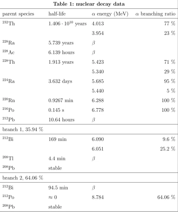
source region target tissue region
detector column decaying nucleus track hitting α the detectors n. 2, 3, 4, 5 0 1 2 3 4 5 z > 0 z < 0 source-tissue separating surface
Fig. 1. Structure of the source-target-detector region. Referring to cartesian coordi-nates x, y, z, the xy-plane is the source-target separating surface (“source boundary” in the text). The source fills the lower half-space (z < 0), while the upper half-space (z > 0) is filled with the target tissue. In the target region we see the detector column (whose central axis coincides with the z-axis). This is a stack of 115 inde-pendent detectors, six of which are visible in the figure. Each detector is a 1 µm3
cube, with center in position (0, 0, 0.5), (0, 0, 1.5), etc.
The range of energies of the α particle of interest here is 1 keV to 9 MeV. In water the maximum energy loss is 2266 MeV cm2
/g (i.e. 0.227 MeV/µm) at E = 0.7−0.75 MeV. This value is the peak energy loss on the left of the minimum of the Bethe-Bloch curve (see for example [14]). The minimum itself would be at much higher energies than 9 MeV. In the range 0.001-9 MeV the distance needed to release a given amount of energy is 2.5-3 times larger in water than in ThO2. With 10 MeV of initial energy, an α track cannot cover more than
40 µm in ThO2 and 115 µm in water. These range values have been used to
determine the size of the implemented source and of the detector column. The modeled source is infinitely extended, but in its practical implementation it is useless to consider source regions from which an emitted particle could never reach the detector.
The physical model is idealized by the 3-dimensional space of points (x, y, z) divided into two regions (see fig.1): for z < 0 we have ThO2 and for z > 0
water.
The implemented source region is a volume ∆x∆y∆z, with ∆x = ∆y = 230 µm, and ∆z = 40 µm. More precisely, the ThO2 source region is:
−115 µm < x < +115 µm, −115 µm < y < +115 µm, −40 µm < x < 0,
The detector column covers 115 µm of z-axis (see fig.1): −0.5 µm < x < +0.5 µm,
−0.5 µm < y < +0.5 µm, 0 < x < 115 µm.
It is divided into 115 cubes, each with volume equal to 1 µm3
. Each of them is an independent detector. This point needs to be stressed: the basic detector is a cube, not the column. The column is a collection of 115 independent detectors, that allow one to use one and the same simulation to evaluate what happens in detectors put at different distances to the source boundary. Both in the target and in the source regions the energy loss by an α particle during its travel is computed to update the particle energy at each step of the simulated trajectory. Inside the detector volume, the energy released in each cubic sub-region and the time of the particle passage are recorded. The steps are short enough to have many steps inside each detector volume.
2.3 Straight trajectories and selection rules.
The reconstruction of the tracks of all the generated particles for 30 years of simulated time would require too much CPU on an ordinary computer, taking also into account that many simulations are needed for fine tuning the code and accumulating statistics. Within some approximations it is possible to reduce much the number of particles whose trajectories are reconstructed by the code.
A key approximation used in this code is that a trajectory is straight. This allows for deciding from the very beginning whether a track will reach the detector or will not.
Generated α particles may be discarded from the very beginning based on the following two decisions made by the algorithm:
a) A particle has insufficient energy to reach any portion of the detector. b) The straight-line extrapolation of the particle trajectory will not cross any detector.
The latter warrants some discussion, because it limits the space precision of the code to 0.1-0.5 µm for the final parts of a reconstructed track.
The quoted databases for the stopping power of the α particles in matter give stopping power and ranges both relative to the projected path (i.e. assuming the same hypothesis of straight-line trajectories used here) and to the length of the real path. A comparison of projected and real ranges [21] of α particles in water shows that their difference is about 0.1 µm at 10 keV compared to a residual range of 0.3 µm, and 0.2 µm at 60 keV compared to a residual range of 1 µm. For larger energies both the true and the projected range increase, but their difference is stable, implying that this difference is built in the last 10-60 keV of energy and that the last 0.3-1 micrometers of trajectory deviate from a straight line.
If this were due to a single deflection at 60 keV, triangle geometry would mean a deviation from the straight line equivalent to 40o, that is a transverse shift of
0.6 µm. This is an extreme case, a standard deflection is considerably smaller. So we estimate an error of 0.1-0.5 µm in the position where the particle comes to rest.
3 Results
3.1 Systematic trends.
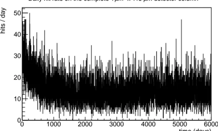
Fig.2 shows the number of α particles that strike the full detector column daily over 30 years. It is possible to distinguish the average trend and its fluc-tuations. The time needed to reach a stationary dose rate (daily fluctuations apart) is about 5 years, that is shorter than the time needed to a thorium source in nature to reach secular equilibrium (a few decades). As noted in [15] this is a consequence of biological depletion.
Fig.3 shows how these hits and the associated energy releases are distributed with respect to the distance to the source-tissue separating surface. The figure reports the cumulative number of hits in one year on each detector of the column, and the total amount of energy released in each detector. In the
region within 70 µm from the source the two histograms are almost exactly proportional, with an average 0.09 ± 0.005 MeV/µm3
of released energy for each hit. The decrease of the hit frequency and the absorbed energy with the distance are almost exactly exponential, and one order of magnitude is lost in 25 µm.
This suggests that, as far as the time-averaged dose absorption is concerned, in presence of a large and compact source the really exposed region of the target is a layer adjacent to the source with thickness of 25 µm.
time (days) 0 1000 2000 3000 4000 5000 6000 hits / day 0 10 20 30 40 50 m detector column µ x 115 2 m µ Daily hit rate on the complete 1
Fig. 2. Daily hit rate for the full detector column (a stack of 115 detectors), simu-lated over a 30 year period.
m) µ detector-source distance ( 0 10 20 30 40 50 60 70 80 ) 3 m µ
) Hit rate (1/ year
3
m
µ
Energy release (MeV / year
-3 10 -2 10 -1 10 1 10 2 10
Hit rate and energy release in a detector as a function of the distance
Fig. 3. Energy release and hit frequency in a detector (a 1 µm3
cube) as a function of the distance between the detector and the source boundary. Continuous histogram: Energy released in each detector in 1 year in stationary conditions (20 years after the beginning of the simulation). Short-dashed histogram: number of hits in each detector in 1 year.
3.2 Fluctuation analysis - general criteria of analysis and relevant space-time scales.
When speaking of “n hits in 24 hours” (in a specified detector) one may refer to two classes of event:
1) The total simulated time (31 years) is divided into 1-day-long bins. Each day begins and ends at midnight and n is the number of hits recorded during that day.
2) A series of n hits may end within 24 hours from its beginning, but these n hits do not necessarily take place in the same day. In this case we may have partially overlapping series of hits.
The former case is easier to handle for statistics. The latter is more relevant for health or safety considerations. Results will be presented for both. The following results are averages from a set of 10 simulations (for the analysis of the events of the class (1)) or 30 simulations (for the analysis of the events of the class (2)). So it is not strange to have results like “0.3 events”. Each simulation is 31-year long, with the exception of the 15-minute-binning case where each simulation covers 10,000 days.
We have to do with three variables, that we name:
“Number of hits” the number of particles incident on a detector in a given time interval.
“Volume”: the volume of the detector where the number of hits is recorded. In this preliminary analysis this is not necessarily 1 µm3
.
“Time interval”: the time interval during which the hits are regrouped together to form a fluctuation, for example 1 day or 1 week. This must not be confused with the much longer duration of the simulation.
We also define “time scale” and “volume scale” the magnitude of the time interval and of the volume.
The number of possible combinations of hit number, time scale and volume scale is rather broad. A numerical simulation should primarily be focused on those combinations for which alternative analytical methods are not well justified. So a relevant preliminary problem is to understand to what extent one may rely upon the Poisson distribution for estimating fluctuations in the number of hits within a given time interval and volume.
in a time interval is constituted by serial decays of one and the same nucleus. An examination of the thorium series shows that we have three critical emis-sion frequencies:
A) 3 decays in a minute, from the sequence of decays224
Ra →220
Rn → 216
Po → 212
Pb.
B) 4 decays in a day, from the sequence 224
Ra → 220 Rn →216 Po → 212 Pb → 208 Pb.
C) 5 decays in a a week, from the sequence of decays 228
Th →224
Ra →220
Rn → 216Po → 212Pb → 208Pb.
Consider the first case as an example. If a detector is hit with an average frequency 4000/day, then we expect a Poisson distribution for the number of hits/day, because these 4000 hits cannot be all serial decays of one and the same nucleus. On the other side, these 4000 hits/day mean 3 hits/minute, and these 3 hits might come from consecutive decays of a single nucleus. The conditions for a safe application of the Poisson statistics are a priori present at the time scale of 1 day, but not at the time scale of 1 minute.
To generalize this example, for the thorium series we define the three critical hit frequencies:
FA = 3/minute ≈ 4000/day,
FB = 4/day,
FC = 5/week ≈ 0.7/day.
with FA >> FB >> FC.
Let F (V ) be the average frequency of hits on a detector of volume V .
If F (V ) >> FA, we expect the Poisson distribution to be a good estimator
for multiple-hit events at all time scales, because F (V ) is much larger than all the critical hit frequencies.
If FB << F (V ) . FA, groups of 2 or 3 events may escape the Poisson
expec-tation on a time scale 1 minute, but for time scales like 1 day or 1 week the Poisson distribution is justified.
If FC << F (V ) . FB, groups of 2, 3 or 4 events may escape the Poisson
expectation on a time scale 1 day or smaller, while for a time scale of 1 week the Poisson expectation is justified.
for time scales up to 1 week. For longer time scales the Poisson expectation is justified.
We have F (1 µm3
) = 40 hits/µm3
year ≈ 0.1 hits/µm3
day for a target region that is in touch with the source (see fig.3). This means that for the assigned source F (1µm3
) < FC < FB < FA.
So, in a detector of volume 1 µm3
we may expect non-Poisson fluctuations on a time scale of 1 week or smaller. However, since F (V ) is an increasing function of V , increasing V over 1 µm3
we will find volumes VC, VB, and VA
such that: F (VC) = FC,
F (VB) = FB,
F (VA) = FA.
If we neglect the dependence of the hit frequency on the distance and assume F (V ) ∝ V , we have
VC = 7 µm 3
(a cube of about 2 µm of edge). Above this volume, the number of events/week follows Poisson expectation.
VB = 40 µm 3
(a cube of 3-4 µm of edge). Above this volume, the number of events/day follows the Poisson expectation.
VA = 40,000 µm 3
(a cube of 0.2 mm of edge). Above this volume, the number of events/minute follows the Poisson distribution.
For these reasons, in the following the reference detector volume will be 1 µm3
. Three different time scales between the code precision limit 15 minutes and the week will be considered.
3.3 Fluctuation analysis - fixed time binning.
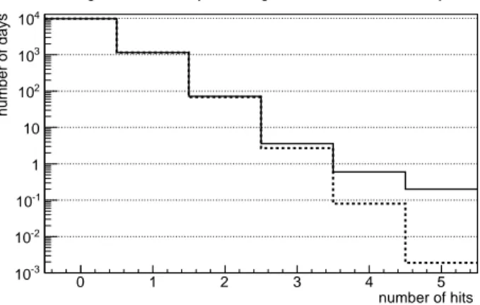
Figure 4 shows the distribution of days with n hits and the corresponding Poisson expectation in the first detector, the one in touch with the source boundary.
A consideration of similar distributions in detectors at larger distances shows that the distribution in the second detector is qualitatively similar to the one of fig.4 but the number of 4-hit and 5-hit events is much smaller (one 5-hit/day event in 10 simulations). For larger distances, only once we find a day with 4 hits (at distance of 4 µm). At all distances, for the frequencies ≤
3 hits/µm3
day the discrepancies between the simulated distribution and the Poisson one are not relevant.
number of hits 0 1 2 3 4 5 number of days -3 10 -2 10 -1 10 1 10 2 10 3 10 4 10
Average number of days with a given number of hits in 30 years
Fig. 4. Continuous histogram: Average number of days with a given number of hits in the first detector in 30 years. The average is calculated over 10 repetitions of the simulation. So, 0.1 is the minimum possible number of days, resulting from one day only in 10 simulations. Short-dashed histogram: the Poisson distribution estimate. Fig.5 shows the distribution of weeks with n hits in the first detector volume. This distribution is close to the Poisson one. The worst disagreement is a factor 3/2 in the case of 5-hit events, the same value at which we find the largest disagreement between the Poisson expectation and the simulated numbers in figure 4. number of hits 0 1 2 3 4 5 6 number of weeks -1 10 1 10 2 10 3 10
Average number of weeks with a given number of hits in 30 years
Fig. 5. Average number of weeks with a given number of hits in the first detec-tor in 30 years. The average is calculated over 10 repetitions of the simulation. Short-dashed histogram: the Poisson distribution estimate.
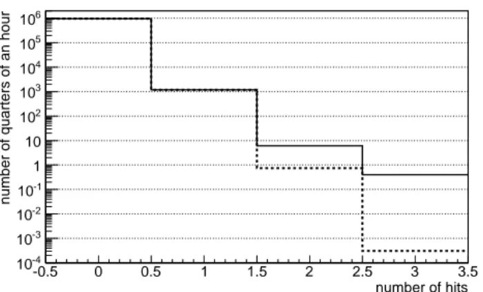
Fig.6 shows the distribution of the hits in 15-minutes periods. Here the number of 2-hit-periods is one order of magnitude larger than the Poisson expectation, and the number of 3-hit-periods several orders of magnitude larger.
The numerical simulations partially confirm what suggested by the preliminary analysis. For 4-hit and 5-hit events on a target with volume equal to 1 µm3
, a day seems a critical time scale, with a frequency of such events that largely
number of hits
-0.5 0 0.5 1 1.5 2 2.5 3 3.5
number of quarters of an hour
-4 10 -3 10 -2 10 -1 10 1 10 2 10 3 10 4 10 5 10 6 10
Average number of quarters of an hour with a given number of hits in 10,000 days
Fig. 6. Average number of 15-minute periods with a given number of hits in the first detector in 10,000 days (slightly more than 27 years). The average is calculated over 10 repetitions of the simulation. Short-dashed histogram: the Poisson distribution estimate.
overcomes the Poisson prediction. Expanding the time scale to 1 week, one arrives to the border of the critical region: the Poisson estimate for such events is almost correct.
The frequencies of 2-hit and 3-hit events are Poisson-like at the 1-day scale. They are larger by orders than the Poisson estimate at the shortest scale allowed by this code, 15 minutes.
3.4 Fluctuation analysis - frequency of “within 24 hours” fluctuations.
For this analysis 30 independent simulations of 30 years each have been per-formed. In these simulations we have found 7 “extreme” and not reciprocally overlapping fluctuations on the 24-hour and 1 µm3
scales:
One 6-hit event within 24 hours and 15 minutes (this involves two overlapping 5-hit series within 24 hours each).
Six 5-hit events within 24 hours (in addition to the previous two events that have been counted as a single 6-hit event).
The above 7 sequences were homogeneously distributed in 30 years. The first years (with a relevant weight of228
Th-initiated chains) did not show a special frequency of many-hit events.
Four of these sequences contained 5 particles emitted by the same nucleus, one contained 2 particles only by the same nucleus, and two sequences con-tained 5 α particles all emitted by different nuclei. Only the two sequences with all the particles emitted by different nuclei would be predicted by the
Poisson distribution, so from another point of view we may confirm that this statistics is inadequate to predict the frequency of days with many hits on the micrometer scale, at small distances from the source.
Only one of the above sequences involved a detector detector that was not the first one of the column, and it was a case where all the hits came from different nuclei. Probably, the relative weight of those events where all the incident particles come from one and the same nucleus decreases with the distance.
4-hit events in 24 hours in 1 µm3
may be found at larger distances. The space distribution of such events in the detector column in 30 years and 30 simulations is (those overlapping with the previous 5-hit and 6-hit events have been excluded):
28 at distance 0-1 µm, 10 at 1-2 µm, 15 at 2-5 µm, 9 at 5-10 µm, 3 at 10-20 µm (the last found event was at 19 µm).
Combining all the events with 4 or more hits would increase the number of events at distance 0-1 µm to 34, and the number of events at distance 1-2 µm to 11. This means that 60 such events out of a total of 72 are within 5 µm of the source, and 69 out of 72 within 10 µm.
4 Conclusions and perspectives
Summarizing the main results:
The time-averaged frequency of hits and the time-averaged released dose de-creases exponentially with the distance from the source-tissue separating sur-face, in such a way that an order of magnitude in the particle and energy flux is lost in about 25 µm from the source. So, if the development of a cancer is associated with single-hit events, the really dangerous region should coincide with this 25-µm-thick layer of tissue that is in touch with the source.
The considered statistics (up to 30 simulations) has allowed analyzing the frequency of events with up to 5 hits within 24 hours in the same target volume. An event with 6 hits have been seen, but just one.
On target regions of size 1 micrometer, events with 4-hit per day and 5-hit per day take place with a frequency that is much larger than predicted by the Poisson statistics. The same is true for events with 3 hits in a much shorter time interval (15 minutes). If the development of a cancer is associated with such multi-hit events, the dangerous region is is a layer of tissue that is in touch with the source, with a thickness that is a decreasing function of the
number of hits. It may be estimated as 1 µm for 5-hit events, 5-10 µm for 4-hit events.
If the time interval is increased to 1 week or more, the Poisson statistics gives good predictions for multi-hit events on target regions with size of 1 µm. The same is expected for a time interval of 1 day if the size of the considered target region is >> 1 µm. Events with 2-3 hits in a minute are expected to overcome Poisson estimates on any target region of sub-visible size.
Further work on the preliminary analysis presented is, of course, required. Most notably, this includes improving the statistics (i.e. the number of simu-lations) of the analysis, for example, to more robustly characterize dependence of many-hit events on distance. Other important refinement would be consid-eration of different source structure and densities and of sparse granular source distributions.
Ethical standards: No human-involving study is reported here.
Conflict of interest statement: None declared.
References
[1] J.D.Abbatt, “History of the use and toxicity of Thorotrast”, Environ. Res.18, 6-12 (1979).
[2] M. Fukumoto and S. Saigusa, “Thorotrast archive and Fukushima Daiichi nuclear power plant Project”, presentation at the “Workshop on Sharing Data & Biomaterials from Radiation Science in Rome”, available at http://fp7store.de/media/Meetings/Rome 2012/10 STORE Rome Fukumoto.pdf [3] H.B.McMahon, A.S.Murphy, and M.Bates, “Endothelial-cell sarchoma of liver
following Thorotrast injections” Amer. J. Path., 23, 585 (1947).
[4] G.Balamurali, D.G. du Plessis, M.Wengoy, N.Bryan, A.Herwadkar, and P.L. Richardson, “Thorotrast-induced primary cerebral angiosarcoma: case report”, Neurosurgery. 2009 Jul;65(1):E210-1;
[5] Y.Yamamoto, N.Usuda, T.Takatsuji, Y.Kuwahara, and M.Fukumoto M., “Long incubation period for the induction of cancer by thorotrast is attributed to the uneven irradiation of liver cells at the microscopic level”, Radiat. Res. 171 494503 (2009).
[6] I. Dos Santos Silva, F. Malveiro, M.E.Jones, and A.J.Swerdlow, “Mortality after radiological investigation with radioactive Thorotrast: A follow-up study of up to fifty years in Portugal”, Radiation Research 159, 52134 (2003).
[7] M.Anderson, K.Juel, and H.H.Storm, “Pattern of mortality among danish thorotrast patients”, Journal of Clinical Epidemiology 46, 637-644 (1993). [8] U. Nyberg, B. Nilsson, L.B.Travis, L.-E.Holm, and P. Hall. “Cancer incidence
among Swedish patients exposed to radioactive Thorotrast: A forty-year follow-up survey”, Radiation Research 157, 41925 (2002).
[9] T.Mori et al, “Summary of entire Japanese Thorotrast follow-up study: updated 1998”. Radiation Research 152 S84-S87 (1999).
[10] N.Becker, D.Liebermann, H.Wesch, G.V.Kaick, “Mortality among Thorotrast-exposed patients and an unThorotrast-exposed comparison group in the German Thorotrast study”, European Journal of Cancer, 1259-1268 (2008).
[11] H. J. Schaefer and A. Golden, “The effectiveness of colloidal Thorium Dioxide as an internal Alpha emitter: a combined morphologic and radioautographic study”, Yale J. Biol Med. 1955 June; 27(6): 432440.
[12] W.E.Strole, and J.N. Wittenberg, N Engl J Med 304 893899 (1981).
[13] Kaul, A. and Noffz, W., “Tissue dose in Thorotrast patients”, Health Phys. 35 113-121 (1978)
[14] G.Friedlander, J.W.Kennedy, E.S.Macias, and J.M.Miller, “Nuclear and radiochemistry”, 3rd ed., (Wiley 1981).
[15] A.Bianconi, M.Corradini, M.Leali, E.Lodi Rizzini, L.Venturelli and N.Zurlo, “Thorotrast: Analysis of the time evolution of its activity concentration, in the 70 years following the chemical purification of Thorium”, Physica Medica: European Journal of Medical Physics 29, Issue 5, 520-530 (2013).
[16] U.Wiedemann, “Manifacture of Thorotrast”, in: The Dosimetry and Toxicity of Thorotrast (IAEA Technical Report 1968), Vienna, International Atomic Energy Agency, pp.1-4.
[17] Y.Yamamoto, J.Chikawa, Y.Uegaki, N.Usuda, Y.Kuwahara, and M.Fukumoto. “Histological type of Thorotrast-induced liver tumors associated with the translocation of deposited radionuclides”, Cancer Sci. 101(2) 336-40 (2010). [18] E.K.Hyde, “The radiochemistry of Thorium” (1960), printed in Nuclear Science
Series, National Academy
of Sciences National Research Council, Subcommittee on Radiochemistry, reprinted by the Technical Information Center, US D.O.E., freely available at www.radiochemistry.org/periodictable/pdf books/pdf/rc000034.pdf
[19] Data tables by the UKDMC (UK Dark Matter Collaboration) at the site http://hepwww.rl.ac.uk/ukdmc/Radioactivity/Th chain/Th chain.html
[20] Chapter 4.5.1 of “Kaye & Laby Tables of Physical & Chemical constants” at the site http://www.kayelaby.npl.co.uk/toc/ cared by NPL (National Physical Laboratory).
[21] Available data tables at the site
http://physics.nist.gov/PhysRefData/Star/Text/ASTAR.html cared by NIST (National Institute of Standards and Technologies).
[22] J.Ziegler, SRIM code and data tables at the site http://www.srim.org [23] W. H. Bragg and R. Kleeman, Philos. Mag. 10, 318 (1905).