DOI: 10.1002/eng2.12060
R E S E A R C H A R T I C L E
Twin-engined diagnosis of discrete-event systems
Nicola Bertoglio
1Gianfranco Lamperti
1Marina Zanella
1Xiangfu Zhao
21Department of Information Engineering, University of Brescia, Brescia, Italy 2College of Mathematics, Physics and Information Engineering, Zhejiang Normal University, Jinhua, China
Correspondence
Gianfranco Lamperti, Department of Information Engineering, University of Brescia, Via Branze 38, 25123 Brescia, Italy. Email: [email protected]
Funding information
Smart4CPPS, Grant/Award Number: POR-FESR 2014-2020 Asse I; National Natural Science Foundation of China, Grant/Award Number: 61972360
Diagnosis of discrete-event systems (DESs) is computationally complex. This is why a variety of knowledge compilation techniques have been proposed, the most notable of them rely on a diagnoser. However, the construction of a diag-noser requires the generation of the whole system space, thereby making the approach impractical even for DESs of moderate size. To avoid total knowledge compilation while preserving efficiency, a twin-engined diagnosis technique is proposed in this paper, which is inspired by the two operational modes of the human mind. If the symptom of the DES is part of the knowledge or experience of the diagnosis engine, then Engine 1 allows for efficient diagnosis. If, instead, the symptom is unknown, then Engine 2 comes into play, which is far less effi-cient than Engine 1. Still, the experience acquired by Engine 2 is then integrated into the symptom dictionary of the DES. This way, if the same diagnosis problem arises anew, then it will be solved by Engine 1 in linear time. The symptom dic-tionary can also be extended by specialized knowledge coming from scenarios, which are the most critical/probable behavioral patterns of the DES, which need to be diagnosed quickly.
K E Y WO R D S
communicating automata, discrete-event systems, knowledge compilation, model-based diagnosis
1
I N T RO D U CT I O N
According to Daniel Kahneman, psychologist and Nobel laureate in Economic Sciences, two modes of thinking coexist in the human brain, which correspond to two systems in the mind, called System 1 and System 2.1System 1operates auto-matically and quickly, with little if any effort, and no sense of voluntary control, such as when orienting to the source of a sudden sound or driving a car in an empty road. By contrast, System 2 operates consciously and slowly, with attention being focused on demanding mental activities, possibly including complex computations or inferences, such as when filling out an intricate application form or checking the validity of a complex argument. Intriguingly, an activity ini-tially performed by System 2, such as driving a car or playing the piano, may be subsequently operated by System 1 after appropriate training.
This “twin-engined” architecture of the mind is a metaphor for the diagnosis approach for discrete-event systems (DESs) presented in this paper. The proposed diagnosis engine (DE) operates in two different modes resembling System 1 and
System 2in the human mind, called Engine 1 and Engine 2. If the diagnosis problem to be solved is part of the knowledge or experience of the DE, then Engine 1 can solve this problem quickly. If, instead, the problem is not part of the knowledge or experience of the DE, then comes into play Engine 2, which requires deep model-based reasoning and, therefore, operates This is an open access article under the terms of the Creative Commons Attribution License, which permits use, distribution and reproduction in any medium, provided the original work is properly cited.
© 2019 The Authors. Engineering Reports Published by John Wiley & Sons Ltd.
Engineering Reports. 2019;1:e12060. wileyonlinelibrary.com/journal/eng2 1 of 20
far more slowly than Engine 1. Still, the experience acquired by Engine 2 in solving the diagnosis problem can be integrated into the knowledge of the DE, so that, in the future, the same diagnosis problem can be solved by Engine 1 efficiently. Besides, the DE is not necessarily born naked, that is, without any knowledge except the model of the DES, otherwise
Engine 2would operate far more frequently than Engine 1 for a possibly long time. Instead, the DE can start working being already equipped with specialized knowledge on domain-dependent scenarios that are considered either most probable or most critical for the safety of the DES (or the surrounding environment) and, as such, need to be coped with efficiently.
2
D I AG N O S I S A N D T H E M Y T H O F TOTA L K N OW L E D G E CO M P I L AT I O N
Diagnosis aims to explain the abnormal behavior of a system based on the observations relevant to its operation, which are perceived from an external observer. In the Artificial Intelligence community, the formal definition of the diagnosis task2led, in the '80s, to the model-based paradigm,3according to which the normal behavior of the system to be diagnosed is described by a model and the diagnosis results have to explain the discrepancies between the output of the system and what we were supposed to observe based on the system model. The diagnosis task generates a collection of sets of faulty components, where each set, named a candidate, is an explanation of the observation. Each candidate explains the observation in the sense that assuming all the components in the candidate are faulty and all the others are normal is consistent with the observation. This model-based diagnosis approach was initially conceived for static systems, such as combinational circuits, and then extended to dynamic systems.Recently, another approach that relies on the exploitation of Artificial Intelligence techniques has been adopted,
data-drivendiagnosis.4,5In fact, machine learning can be used to automatically process sensor data and create models for fault prediction and classification. Typically, nominal data (ie, data relevant to the normal behavior) and data from different faults can be used to train fault classifiers. This relieves the diagnostician from the burden of creating a model of the system/process to be diagnosed, sometimes even from the burden of identifying proper features since deep learn-ing techniques offer potential tools for automatic feature extraction from (physical) signals.6However, in many industrial applications, faults are rare events and available training data from faulty conditions is usually limited.7Hence, collecting a sufficient amount of data from relevant faulty situations for data-driven diagnosis is a time-consuming and expensive process.
Alternatively, the behavior of the system to be diagnosed can be described as a set of cases, where each case is labeled as either normal or faulty. The case base can include the diagnostician's expertise, starting from a limited amount of cases (that is, an incomplete knowledge), and its size can increase incrementally over time, as such an expertise is growing. The human diagnostician is assisted in decision making about diagnosis, maintenance and reconfiguration by the interactive case-based reasoning system, for instance in dealing with automated production systems.8
In some contexts, such as rotating machinery, which is among the most important equipments in modern industry, fault diagnosis can be regarded as a pattern recognition problem. Due to the variability and richness of the response sig-nals relevant to the rotating machinery condition, it is almost impossible to recognize fault patterns directly: Artificial Intelligence techniques, encompassing a preprocessing step for feature extraction and an online step for fault recogni-tion, are very promising.9Specifically, several methods have been used for performing the latter step, including convex optimization, mathematical optimization, as well as classification, statistical learning, and probability-based algorithms. An advantage of model-based methods, with respect to data-driven methods, is that fault detection and isolation can be achieved without the need for data from different faults. In this paper, we deal with a model-based approach as applied to dynamical systems. For a dynamical system, a DES10 model can be adopted. This model can be described as a Petri net,11,12or as a finite automaton, where each state of the automaton represents a state of the dynamical system (at some abstraction level), like in this paper. The model is typically distributed, consisting of several automata that communicate with one another.13 Each automaton represents the behavior of a component, which is a DES itself, where some state transitions are faulty (and, as such, each of them is marked with a fault) and the occurrence of some transitions can be perceived from the outside of the system (and, as such, each of these transitions is marked with an observable event). Diagnosing a DES means finding out all the candidates relevant to a given sequence of observed events, where a candidate is a set of faults that can explain such a sequence.
Model-based diagnosis of DESs represented as networks of finite automata is grounded on the seminal work of Sampath et al,14-16which, as relying on a compiled-knowledge data structure called a diagnoser, has been coined the
diagnoser, which is then exploited online to draw the candidates relevant to any given sequence of observed events. Two major requirements are assumed by the diagnosis method embodied in the diagnoser approach.
• To guarantee the soundness and completeness of the diagnosis results, the DES must have a property called
diagnos-ability.
• To generate the diagnoser, the materialization of the whole behavior space of the DES is needed.
These requirements are strongly interrelated as the creation of the whole behavior space is needed not only for fulfilling the second requirement (as the diagnoser is drawn from the system behavioral space) but also for checking whether the first requirement is met (that is, for performing the diagnosability analysis). However, the materialization of the whole behavioral space is most critical since, even for DESs of moderate size, the behavior space may become overwhelmingly large, being exponential in the number of components. The memory demands for such a space are difficult to satisfy, and producing it is a computationally expensive and inefficient process (see, for instance, the work of Rozé17about the computational difficulties of the diagnoser approach, or the worst case computational complexity analysis in the work of Baroni et al,18 or the discussions in the works of Basile11 and Kurien and Nayak19). Nowadays, the diagnoser approach can still be regarded as a reference conceptual framework for the definition of both the task of diagnosis and the notion of diagnosability of DESs described as networks of finite automata. However, from an operational point of view, subsequent contributions in the literature about diagnosis and/or diagnosability of DESs described as networks of finite automata do not follow the original diagnoser approach method as the awareness has soon grown that total knowledge compilation is definitely a myth.
Notwithstanding the computational drawbacks of the diagnoser approach, the topic of diagnosability has unsurpris-ingly received considerable attention in the literature. In the work of Sampath et al,14 the property of diagnosability is defined for (partially observable) DESs, whose prefix-closed language of the events is live and does not include any cycle of unobservable events. Roughly, a system is diagnosable if, given any occurrence of any failure event, it is pos-sible to detect and isolate that failure within a finite number of events (ie, a finite number of transitions of the system model) following it. In other words, the system is diagnosable if it is always possible to detect within a finite delay the occurrence of a failure event (and uniquely identify its type) by using the record of observed events. A necessary and suf-ficient condition is proposed in the work of Sampath et al14to check diagnosability based on the diagnoser construction. However, testing diagnosability is performed in polynomial time in the cardinality of the state space of the diagnoser, which, in the worst case, is exponential in the cardinality of the state space of the system model. The most famous approach to checking whether the diagnosability property holds for a given DES is the twin plant method,20whose time complexity is polynomial in the global number of the states of the system model. In fact, this method relies on the construction of the twin plant, this being the synchronous product of a nondeterministic finite automaton (or NFA, drawn from the global model of the DES, and generating the DES observable language) by itself over the alphabet of observable events. A similar approach to diagnosability checking, whose complexity is still polynomial in the number of states of the global behavioral space, is presented in the work of Yoo and Lafortune.21Finding out whether the condition for diagnosability (as restated by the twin plant method) holds was formulated also as a model-checking problem22,23or a satisfiability problem.24
In the work of Console et al,25the analogy between modeling concurrent processes (for the purpose of performance evaluation) and modeling distributed physical systems (for the purpose of diagnosis and diagnosability analysis) is pointed out. The concepts of diagnosis and diagnosability are then characterized based on a process algebra formalism (PEPA).
Most of existing works focused on how to verify that the intrinsic diagnosability of a DES assume that candidates are computed by a diagnostic algorithm that takes as input a completely certain sequence of observable events. The ability to disambiguate DES candidates for a system with uncertain observations is discussed in the work of Su et al.26 The uncertainty is measured by a parameter, which allows for studying the level of noise that can affect the observed sequence of events without impacting the performance of diagnosis. A definition of DES diagnosability that extends the original one14is provided, as well as a method to check whether the newly defined property holds for a given DES. This method extends the original twin plant method20by considering two kinds of uncertainty in the sequence of observable events.
Diagnosability of fuzzy DESs (FDESs), namely, fuzzy diagnosability, is faced in the work of Liu and Qiu.27The FDESs are DESs whose states and events, instead of being crisp, are fuzzy (according to the fuzzy set theory) to represent the vagueness, impreciseness, and subjectivity that are typical features in several real-world domains, such as biomedicine. Specifically, in the quoted paper, FDESs are modeled as max-min systems, and observability is assumed to be fuzzy. A fuzzy diagnosability function to characterize the diagnosability degree of a FDES is introduced, a necessary and sufficient condition for diagnosability of FDESs, which generalizes that for crisp DESs introduced in the work of Sampath et al,14
is presented, and a method to check the fuzzy diagnosability of FDESs is given that is based on the diagnoser in the aforementioned work.14
In the work of Paoli and Lafortune,28 the property of diagnosability for DESs tailored as hierarchical finite state machines (HFSMs) is introduced. According to this notion, a fault can be detected using only a high-level description of the HFSM, and diagnosability can be tested by relying on a so-called extended diagnoser. If some sufficient conditions hold, the extended diagnoser can be built from particular projections of the HFSM. For faults that cannot be proven to be diagnosable in an HFSM using the aforementioned projections, if another sufficient condition holds, a refined version of the diagnoser can be used. The whole approach is aimed at checking diagnosability while avoiding the construction of the behavioral model of the whole system, as instead required by both the diagnoser approach and the twin plant method.
In order to avoid the construction of the behavioral model of the whole system, another research line performs a dis-tributed diagnosability analysis.29,30Basically, by taking advantage of the distributed modeling of the considered DES, a (small) local twin plant is built for each component, instead of building a (huge) twin plant relevant to the whole DES. Local twin plants are then synchronized with each other until diagnosability is decided. Unfortunately, the synchroniza-tion of local twin plants can remain a bottleneck for large systems. The scalability of the approach is increased in the work of Schumann and Huang,31where DES components (and their relevant local twin plants) are organized into a join-tree, a classical tool adopted in various fields of Artificial Intelligence. Once the jointree has been constructed, only the twin plants in each jointree node need to be synchronized, and all the remaining computation takes the form of message passing along the edges of the jointree.
Fault detection in DESs was generalized32to the recognition of a pattern, which can represent the occurrence of a single fault as well as of multiple faults, the ordered occurrence of significant events, the multiple occurrences of the same fault, etc. Consequently, the notion of fault diagnosability was generalized to pattern diagnosability, and the task of checking pattern diagnosability was faced in a distributed way.33
Diagnosability analysis was addressed for DESs represented as labeled Petri nets also, both bounded34,35 and unbounded.36
Coming back to the diagnosis task, as already remarked, solving a DES diagnosis problem instance means finding out all the sets of faults entailed by the system evolutions that produce the sequence of events that have been observed. Based on the method for tracking the evolutions of the system that explain a given sequence of observable events, two approaches to diagnosis of DESs were singled out in the work of Basile.11
• The former, coined compiled diagnoser, generates offline (a concise model of) all possible evolutions and then retrieves online only the evolutions that explain the observation; it basically consists in the diagnoser approach.14,15
• The latter, coined interpreted diagnoser, generates online in one shot the evolutions, explaining the sequence of obser-vations; this is traditionally the case with the so-called active system approach by the authors,18,37-41and the works that stem from it.42,43
Offline computation means preprocessing, which is a computation performed when no diagnostic processing is ongo-ing: it generates compiled knowledge once and for all, with this knowledge being possibly exploited online several times. The offline computation as well as the space requirements of the methods in the former approach are prohibitive, whereas the online computation to solve a diagnosis problem instance is quite efficient (a sequence of observable events is pro-cessed in linear time in the length of the sequence itself). The methods in the latter category do not perform any offline computation, they only carry out an online model-based reasoning, whose high cost is limited as it is focused on a single sequence of observable events. Still, this alternative “diagnoserless” approach comes with a significant cost in computa-tion because of the extended model-based reasoning required. Therefore, shall we abandon the idea of diagnosing DESs efficiently?
In order to face this question, recent work by the authors has tried to combine the two mentioned approaches and to make them cooperate with each other, both for a posteriori diagnosis44and diagnosis during monitoring45: this paper moves a further step in this direction as far as a posteriori diagnosis is concerned. The main findings can be summarized as follows.
• The notion of a symptom dictionary, this being a compiled knowledge structure for a posteriori diagnosis, is defined. • A method for performing a posteriori diagnosis that is based on an (extensible) portion of the symptom dictionary that
includes its initial state, called open (symptom) dictionary, is presented.
• The notion of a symptom pattern, this being a deterministic finite automaton (DFA) that recognizes the language consisting of some symptoms of the considered DES, is introduced.
• The way a scenario, which is an NFA representing some behaviors of interest (the most likely or the most critical ones), can be processed so as to draw its corresponding symptom pattern is shown.
• The pseudocode of an algorithm for extending the open (symptom) dictionary based on a symptom pattern is provided. Using the terminology of Section 1, the open (symptom) dictionary is the repository of the compiled knowledge exploited by Engine 1, where this knowledge can be incomplete. If the compiled knowledge is insufficient to solve a new diagnosis problem, an online computation is performed, that is, Engine 2 is run, so as to (permanently) add to the dictio-nary the chunks of knowledge that are missing inherently to such a problem. The diagnosis method is sound and complete although the compiled knowledge is incomplete since it is able to generate the needed chunks of compiled knowledge on the fly (by drawing them from the “raw” knowledge in the DES component models and in the DES topology). After a problem has been solved inefficiently (by Engine 2) once, it will be solved efficiently (by Engine 1) thereafter. In previous work relevant to the interpreted diagnoser, instead, each diagnosis problem was solved anew every time. Moreover, the added chunks of compiled knowledge can enable Engine 1 to solve efficiently several additional problems besides the one that has spurred the open (symptom) dictionary extension.
3
D E S S A N D D I AG N O S I S P RO B L E M S
A DES is assumed to be a network of components, where each component, endowed with input and output pins, is modeled as a communicating automaton.13Each output pin of a component is connected with an input pin of another component by a link. The way a transition is triggered in a component is threefold: (1) spontaneously (by the empty event𝜀), (2) by an (external) event coming from the extern of the DES, or (3) by an (internal) event coming from another component of the DES. When a component performs a transition based on a (possibly empty) input event e, it may generate a set E of new events on its output pins, which possibly trigger the transitions of other components, with the triggering events being consumed. This cascading process continues until the DES becomes quiescent anew. A transition generating an event on an output pin can occur only if this pin is not occupied by another event already. Assuming that only one component transition at a time can occur (asynchronism), the process that moves a DES from the initial quiescent state to the final quiescent state can be represented by a sequence of component transitions, called a trajectory of the DES. At the occurrence of each transition, a DES changes state, with each state x of being a pair (C, L), where C is the array of current states of components and L is the array of (possibly empty) current events placed in links. Formally, the (possibly infinite) set of trajectories of is specified by a DFA, namely, the space of ,
∗ = (Σ, X, 𝜏, x
0, Xf), (1)
where Σ (the alphabet) is the set of component transitions, X is the set of states,𝜏 is the (deterministic) transition function,
𝜏 ∶ X × Σ → X, x0is the initial (quiescent) state, and Xfis the set of final states. A state (C, L) of is final when all links in
Lare empty (no event is placed in the links). The DES model adopted does not make any assumption about the liveliness of the language of events/transitions of the DES. Moreover, the space of the DES may include unobservable cycles.*
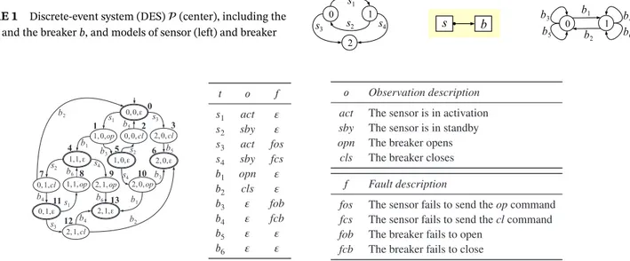
Example 1. Outlined in the center of Figure 1 is a DES called (protection), which includes two components, a sensor s and a breaker b, and one link connecting the (single) output pin of s with the (single) input pin of b. The model of the sensor s (outlined on the left side of Figure 1) involves three states (denoted by circles) and four transitions (denoted by arcs). The model of the breaker b (outlined on the right side of Figure 1) involves two states and six transitions. No final states are defined for component models. Each component transition t from a state p to a state p′, triggered by an input event e, and generating a set of output events E, is denoted by the angled triple t =⟨p, (e, E), p′⟩, as detailed in Table 1.†The space of, namely, ∗, is depicted on the left side of Figure 2, where each state is identified by a triple (ss, sb, e), with ssbeing the state of the sensor, sbthe state of the breaker, and e the internal event in the
link (𝜀 means no event). The initial state is (0, 0, 𝜀); final states are double circled. To ease referencing, the states of are renamed by numbers 0 · · · 12. Owing to cycles, the set of possible trajectories of is infinite, one of them being
*An unobservable cycle makes the DES undiagnosable when it translates into a so-called indeterminate hidden cycle within the special diagnoser intro-duced in the work of Basilio and Lafortune.46However, the diagnosis method described in the paper (and the active system approach in general) is not affected by the possible non diagnosability induced by unobservable cycles, as it copes with both diagnosable and undiagnosable DESs the same way. †As such, the alphabet of the automaton model is a set of pairs(e,E),where e is the (possibly empty) input event and E is the (possibly empty) set of output events.
TABLE 1 Transition details for the components s and b of the discrete-event system (DES) outlined in Figure 1
Transition Description
s1=⟨0, (ko, {op}), 1⟩ The sensor s detects a threatening event ko and generates the op (open) output event s2=⟨1, (ok, {cl}), 0⟩ The sensor s detects a liberating event ok and generates the cl (close) output event s3=⟨0, (ko, {cl}, 2⟩ The sensor s detects a threatening event ko, yet generates the cl (close) output event s4=⟨1, (ok, {op}), 2⟩ The sensor s detects a liberating event ok, yet generates the op (open) output event b1=⟨0, (op, ∅), 1⟩ The breaker b reacts to the op (open) input event by opening
b2=⟨1, (cl, ∅), 0⟩ The breaker b reacts to the cl (close) input event by closing
b3=⟨0, (op, ∅), 0⟩ The breaker b does not react to the op (open) input event and remains closed b4=⟨1, (cl, ∅), 1⟩ The breaker b does not react to the cl (close) input event and remains open b5=⟨0, (cl, ∅), 0⟩ The breaker b reacts to the cl (close) input event by remaining closed b6=⟨1, (op, ∅), 1⟩ The breaker b reacts to the op (open) input event by remaining open
FIGURE 1 Discrete-event system (DES) (center), including the sensor s and the breaker b, and models of sensor (left) and breaker (right)
FIGURE 2 From left to right: space∗, mapping table𝜇(), and observation (top) and fault (bottom) descriptions
[s1, b1, s2, b4], which ends in state 11, described as follows: s detects a threatening event and commands b to open;
bopens; s detects a liberating event and commands b to close; eventually, however, b does not close.
For diagnosis purposes, we characterize a DES with its observability (whether each transition is observable or unob-servable) and normality (whether each transition is normal or faulty). No assumption is made about the nature of faults: each individual fault can either be permanent or not, independently of the other faults.
Let T be the set of component transitions in, O a finite set of observations, and F a finite set of faults. The mapping
table𝜇 of is a function
𝜇() ∶ T → (O ∪ {𝜀}) × (F ∪ {𝜀}, (2)
where𝜀 is the empty symbol. Table 𝜇() can be represented as a finite set of triples (t, o, f ), where t ∈ T, o ∈ O ∪ {𝜀}, and f ∈ F ∪ {𝜀}. The triple (t, o, f ) defines the observability and normality of t: if o ≠ 𝜀, then t is observable, else t is
unobservable;‡if f≠ 𝜀, then t is faulty, else t is normal.
Based on𝜇(), each trajectory T in ∗ can be associated with a symptom and a diagnosis. The symptom of T is the finite sequence of observations involved in T,
= [o|t ∈ T, (t, o, 𝑓) ∈ 𝜇(), o ≠ 𝜀]. (3)
‡In a physical DES, an observable transition manifests itself to an external observer by the generation of the observation associated with it (when the transition is triggered). In other words, if the transition is observable, then its occurrence generates the observation; otherwise (if the transition is unobservable), no observation is generated.
The diagnosis𝛿 of T is the finite set of faults involved in T, ie,
𝛿 = {𝑓 |t ∈ T, (t, o, 𝑓) ∈ 𝜇(), 𝑓 ≠ 𝜀}. (4)
Since a diagnosis is a set, only one instance of each fault f can be in𝛿. Hence, the domain of possible diagnoses is bounded by the (finite) powerset 2F. By contrast, several instances of the same observation o can be in symptom; therefore, the domain of possible symptoms is in general infinite. Trajectory T involved in Equation (3) is said to imply, denoted
T⇒ . Likewise, trajectory T involved in Equation (4) is said to imply 𝛿, denoted T ⇒ 𝛿. A trajectory of is observed as a
symptom and, since the observed symptom can be implied by several (possibly infinite§) trajectories, several diagnoses can be associated with the same symptom, which are collectively called the explanation of the symptom. Let be a symptom of. The explanation Δ of is the finite set
Δ() = {𝛿 |T ∈ ∗, T ⇒ , T ⇒ 𝛿}. (5)
That is, the explanation of is the set of diagnoses (called candidates) implied by the trajectories of that imply . It is worth remarking that a trajectory implying a given symptom does not necessarily end with an observable transition. In fact, in a trajectory in Equation (5), the transition generating the last observable event in can be followed by unobservable transitions. In other words, the candidates produced by the diagnosis method presented in this paper (and in the active system approach in general) do not account solely for trajectories generating the given symptom and ending with an observable transition (as is the case with the diagnoser approach14) but also for trajectories generating the given symptom and ending with (a chain of) unobservable transitions, possibly involving unobservable cycles.
Example 2. With reference to the DES introduced in Example 1, displayed on the center of Figure 2 is the mapping table𝜇(), where the symbols are described on the right side of the figure, namely, the observations (top) and the faults (bottom). Let = [act, opn, sby] be a symptom of . Based on ∗in Figure 2, two trajectories imply, namely,
T1 = [s1, b1, s2, b4]and T2 = [s1, b1, s4, b6], where T1involves the faulty transition b4, whereas T2involves the faulty transition s4. Hence, the explanation of includes two (singleton) candidates, namely, Δ() = {{fcb}, {fcs}}. In plain words, two scenarios are possible: either the breaker failed to close ( fcb) or the sensor failed to send the closing command ( fcs).
In theory, it is always possible to generate online the explanation of a symptom of by abducing the subspace of ∗ involving all and only the trajectories implying. However, the application domain may require the explanation to be given under stringent time constraints, thereby making this process impractical. In theory (and ideally), we could generate offline a data structure representing all possible symptoms of and associating with each symptom the corresponding explanation. This way, given a symptom, the explanation could be immediately known online from the data structure.
4
S Y M P TO M D I CT I O NA RY
In this section, we present a technique for preprocessing a DES to generate a data structure, called the symptom dictionary, which associates each possible symptom of the DES with the corresponding explanation. Still, it should be clear that the symptom dictionary is introduced for formal reasons only and is never materialized (completely). To this end, we first introduce the notion of an extended space.
Definition 1. Let∗= (Σ, X, 𝜏, x
0, Xf)be the space of a DES, and F the domain of faults within the mapping table
𝜇(). The extended space of is a DFA
+= (Σ, X+, 𝜏+, x+
0, Xf+), (6)
where Σ is the alphabet (the same as in∗), X+is the set of states (x, 𝛿), x ∈ X, 𝛿 ⊆ F; x+
0 = (x0, ∅); Xf+is the set of final states (x, 𝛿), where x ∈ Xf;𝜏+∶X+× Σ→ X+is the transition function, where𝜏+((x, 𝛿), t) = (x′, 𝛿′)iff𝜏(x, t) = x′and
𝛿′=𝛿 ∪ {f} if (t, o, 𝑓) ∈ 𝜇(), 𝑓 ≠ 𝜀 (when t is faulty), otherwise 𝛿′=𝛿 (when t is normal).
§If a trajectory implies a symptom and includes a cycle with no observable component transitions, then there is an unbounded number of trajectories implying this symptom, each one is obtained by iterating the cycle a different number of times. However, since the diagnosis of a trajectory is a set of faults (without duplicates), additional iterations of the same cycle do not extend the diagnosis with new faults.
Proposition 1. The regular language¶of+equals the regular language of∗.# Besides, if x+= (x, 𝛿) is a state in +,
then the following two properties hold: (1) for each trajectory T in∗ending in x, there is a trajectory T+in+ending in
x+such that T+=T and T⇒ 𝛿; and (2) for each trajectory T+in+ending in x+, there is a trajectory T in∗ending in
x such that T = T+and T⇒ 𝛿.
Proof. First, we prove that the regular language of+equals the regular language of∗. (Soundness) If T ∈+, then
T ∈∗. The proof is by induction on the sequence of transitions in T. (Basis) Trivially, if T
0= [ ] ∈+, then T0∈∗. (Induction) If a prefix Ti= [t1, … , ti] ∈+and Ti∈∗, then, if Ti+1 = [t1, … , ti, ti+1] ∈+, then Ti+1∈∗. In fact, the state reached by Tiin+, namely, x+i = (xi, 𝛿i), is such that xiis the state reached by Tiin∗, as the sequence
of component transitions in Tiis the same in both+and∗. Hence, if ti+1is triggerable in x+i, then it is triggerable in xialso, as the triggerability of ti+1depends on xionly. (Completeness) If T ∈ ∗, then T ∈ +. Again, the proof
is by induction on the sequence of transitions in T. (Basis) Trivially, if T0 = [ ] ∈ ∗, then T0 ∈ +. (Induction) If a prefix Ti = [t1, … , ti] ∈ ∗ and Ti ∈ +, then if Ti+1 = [t1, … , ti, ti+1] ∈ ∗, then Ti+1 ∈ +. In fact, if xiis the
state reached by Tiin∗, then the state reached by Tiin+will be xi+ = (xi, 𝛿i). Therefore, if ti+1is triggerable in xi,
then it is triggerable in x+
i also, as the triggerability of ti+1depends on xionly. In other words,
+has the same regular language as∗. Then, we prove property (1) of the proposition. Assume T = [t
1, … , tn] ∈∗ending in xn. Since X∗
and+share the same regular language, there is a trajectory T+ =Tin+ending in x+
n = (xn, 𝛿n), as the sequence
of component transitions in T is the same as in T+. Moreover, T⇒ 𝛿, as, according to Definition 1, 𝛿 is constructed by accumulating the set of (nonempty) faults associated with the transitions in T. Finally, we prove property (2) of the proposition. Assume T+ = [t
1, … , tn] ∈ +ending in x+ = (xn, 𝛿n). Since X+and∗ share the same regular
language, there is a trajectory T = T+in∗ending in x
n, as the sequence of component transitions in T is the same as
in T+. Moreover, T⇒ 𝛿, as, according to Definition 1, 𝛿 is constructed by accumulating the set of (nonempty) faults associated with the transitions in T. This concludes the proof of Proposition 1.
Example 3. With reference to the DES in Example 1, displayed in Figure 3 is the extended space +, with states renamed by numbers 0 · · · 47 and final states double circled. In accordance with Proposition 1, comparing the extended space+with the space∗displayed in Figure 2, it turns out that the regular language of+equals the regular language of∗. Besides, in accordance with property (1) of the proposition, considering the trajectory
T = [s1, b1, s2, b4, s3, b2] in∗, which ends in state 6, there is a trajectory T+ = Tin + that ends in the state 18 = (6, { fcb, fos}) such that T ⇒ { fcb, fos}. Moreover, in accordance with property (2) of the proposition, consid-ering the trajectory T+ = [s1, b1, s2, b4, s1, b6, s2, b2, s3, b5]in+, which ends in state 18 = (6, { fcb, fos}), there is a trajectory T = T+in∗that ends in state 6 such that T⇒ { fcb, fos}.
Definition 2. Let+be an extended space. Let+
n be the NFA obtained from+by substituting the symbol t (com-ponent transition), marking each transition in+, with the (possibly empty) observation o, where (t, o, 𝑓) ∈ 𝜇().‖ The symptom dictionary of is the DFA ⊕obtained by determinization ofn+, where each final state x⊕of⊕is marked with the set of diagnoses associated with the final states of+
n included**in x⊕, denoted Δ(x⊕).
Proposition 2. The regular language of⊕is equal to the set of possible symptoms of. Besides, if is a symptom with accepting state x⊕in⊕, then Δ(x⊕) = Δ().
Proof. First, we prove that the regular language of the symptom dictionary⊕is equal to the set of symptoms of. Notice that, since⊕is obtained by determinization of the NFA+
n, it suffices to show that the language ofn+ is equal to the set of symptoms of. (Soundness) If ∈ +
n, then is a symptom of . In fact, according to Definition 2, = [o|(t, o, 𝑓) ∈ 𝜇(), o ≠ 𝜀], where t is the component transition marking an arc in +. Based on Proposition 1, the sequence of such component transitions, namely, the corresponding trajectory T+, is a trajectory in∗ also. Hence, according to Equation (3), is a symptom of . (Completeness) If is a symptom of , then ∈ n+. In fact, by
¶The regular language of a finite automaton(be it deterministic or nondeterministic) is the set of strings accepted (recognized) by.47 #Hence, the notion of a trajectory is applicable to the strings in the regular language of+also.
‖The substitution of the component transition t with the observation o associated in the mapping table yields in general an NFA (namely,+ n) because of two reasons:(1)the observation o may be the empty symbol𝜀, and(2)there may be two arcs exiting the same state that are marked with the same observation o.
FIGURE 3 Extended space+
definition of a symptom, there is a trajectory T ∈∗, where = [o|(t, o, 𝑓) ∈ 𝜇(), o ≠ 𝜀]. By virtue of Proposition 1,
T ∈ +. Hence, after the transformation of+ into+
n in Definition 2, T is mapped to [o|(t, o, 𝑓) ∈ 𝜇(), o ≠ 𝜀], namely,. In other words, ∈ +
n.
Now, we show that, if is a symptom with accepting state x⊕in⊕, then Δ(x⊕) = Δ(). First, if 𝛿 ∈ Δ(x⊕), then
𝛿 ∈ Δ(). In fact, based on Definition 2, there is a final state x+= (x, 𝛿) in +such that x is final in∗. According to Proposition 1, there is a trajectory T ∈∗such that T⇒ 𝛿. Moreover, since x⊕is the accepting state of, T ⇒ . In other words, based on Equation (5),𝛿 ∈ Δ(). Second, if 𝛿 ∈ Δ(), then 𝛿 ∈ Δ(x⊕). In fact, based on Equation (5), there is T ∈ ∗such that T ⇒ and T ⇒ 𝛿. According to Proposition 1, T ∈ +. Hence, there is a (final) state
x+ = (x, 𝛿) in +such that x is the (final) state reached by T in∗. Based on Definition 2, when+is transformed into+
n, the trajectory T is transformed into a sequence of observations that, once the𝜀 symbols are removed, equals , with accepting state x+.
To conclude the proof, it suffices to show that x+∈x⊕. This comes from the mode in which the Subset Construction
determinization algorithm operates: if a string s in accepted by an NFA in a state n, then the accepting state d of s in the DFA (equivalent to the NFA) generated by Subset Construction includes n. The proof is by induction on the string
s. (Basis) If s is empty, then the accepting state n of s belongs to the𝜀-closure of the initial state n0. Since the initial state of the DFA is in fact the𝜀-closure of n0, the NFA state n belongs to the initial state of the DFA, which is in fact the accepting state of the empty string. (Induction) If n is the accepting state of a string s in the NFA and n belongs to the accepting state d of the DFA, then, if n′is the accepting state of the extended string s′=s ∪ [o]in the NFA, then n′ belongs to the accepting state d′of s′in the DFA. In fact, n′is necessarily reached by a sequence of transitions of the NFA (exiting n) that involves just the symbol o. Therefore, all the NFA states preceding the transition marked by o in such a sequence will belong to the DFA state d, whereas n′will belong to the𝜀-closure of the set of states reached by the transitions exiting the states of d that are marked by o, which, based on Subset Construction, are in fact the set of states belonging to d′. Hence, n′belongs to d′. This concludes the proof of Proposition 2.
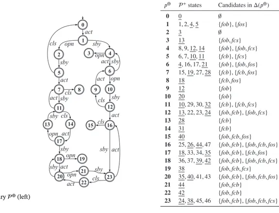
Example 4. With reference to+in Figure 3, the symptom dictionary⊕is outlined on the left side of Figure 4. Incidentally, all states in⊕are final. On the right side of Figure 4, each state p⊕of⊕is described in terms of the +states included in p⊕(with the final states being underlined) and the associated set of diagnoses, which, based on
FIGURE 4 Symptom dictionary⊕(left) and relevant state details (right)
Proposition 2, is in fact the explanation of each symptom with accepting state p⊕. In accordance with Proposition 2, one can take any string in the regular language of⊕and find out that this string is a symptom of by considering the trajectories in the space∗ displayed in Figure 2. For instance, the string [act, opn, sby] in ⊕is the symptom relevant to two trajectories of, namely, T1 = [s1, b1, s2, b4]and T2 = [s1, b1, s4, b6](cf Example 2). Moreover, still in accordance with Proposition 2, considering again the symptom = [act, opn, sby], which has accepting state 5 in ⊕, we have Δ(5) = {{ fcb}, { fcs}}, which in fact equals the explanation Δ() determined in Example 2.
A symptom dictionary⊕is an extremely efficient tool for a posteriori diagnosis of DESs, where candidates are gener-ated after the reception of the complete symptom. Given a symptom, the computation of Δ() boils down to matching ⊕ against, a simple operation with complexity that is linear in the length of . In theory, the symptom dictionary
allows the DE to operate always in quick mode by Engine 1, with Engine 2 never coming into play. However, as recalled in Section 2, like for the diagnoser, the symptom dictionary requires total knowledge compilation, which is out of dispute. Therefore, in order to escape from the myth of total knowledge compilation and somewhat retaining the advantage of
Engine 1, we propose a restricted dictionary that expands over time either by the “experience” acquired from the solution of new problems or by the injection of specific knowledge. In other words, we propose an open dictionary.
5
O P E N D I C T I O NA RY
Roughly, an open dictionary is a subgraph of the symptom dictionary. Hence, the (regular) language of an open dictionary is a subset of the (regular) language of the symptom dictionary, which, based on Proposition 2, is the set of symptoms of the DES. This means that only a (possibly tiny) fraction of the symptoms of the DES are cataloged in the open dictionary. Still, each symptom that is cataloged in the open dictionary is associated with exactly Δ(), the sound and complete set of candidates that explain. Hence, despite being sound (but not complete) in the set of symptoms (as it contains only a subset of the symptoms of the DES), the open dictionary is sound and complete in the explanation of the symptom, pro-vided that the symptom is included in the language of the open dictionary.††What is the initial configuration of the open
††It is like having an “open” dictionary of the English language that contains only a subset of the English words. Still, each English word that is included in the open dictionary is explained exactly as it is in the (complete) English dictionary. In that sense, the open English dictionary is sound in the explanation of the words included, yet incomplete in the words of the English language. Therefore, “openness” refers to the set of words cataloged, not to the explanation of these words.
FIGURE 5 Prefix[2]⊕of the symptom dictionary⊕
dictionary? Although the open dictionary can be initially empty, we suggest to initialize it with a prefix of the symptom dictionary, as specified in Definition 3.
Definition 3. Let⊕be a symptom dictionary. The distance of a state x⊕in⊕is the minimum number of transitions connecting the initial state of⊕with x⊕. The prefix of⊕up to a distance d ≥ 0, denoted [⊕d], is the subgraph of ⊕comprehending all the states at a distance≤ d and all the transitions along paths (starting from the initial state of
the symptom dictionary) that have length≤ d.
Example 5. With reference to Figure 4, the prefix of⊕up to distance 2, namely, [2]⊕, is displayed in Figure 5 (cf Figure 4 for state details).
A prefix⊕
[d]provides the explanation of every symptom that is not longer than d. If ⊕
[d]embodies a cycle (which is
not the case in[2]⊕), it also provides the explanation of the infinite set of symptoms encompassing this cycle. However, any symptom longer than d may not belong to the language of⊕
[d], such as = [act, sby, opn] in ⊕
[2]. In this case, comes into play Engine 2, which generates the explanation Δ() based on the abduction of , namely, a DFA whose language is the subset of the trajectories of implying . To this end, Engine 2 performs model-based reasoning to reconstruct the subspace of∗required. Once provided the explanation Δ(), the “experience” acquired by the DE can be integrated into the open dictionary based on the symptom pattern of. However, the notion of a symptom pattern goes beyond a (plain) symptom, as specified below.
Definition 4. A symptom pattern of a DES is a DFA whose alphabet is the set of observations of . A string in the language of the symptom pattern that is not a symptom of is a spurious symptom.
A special (and very simple) case of symptom pattern is associated with each symptom, denoted ∗, which is the DFA recognizing (the language of ∗is the singleton {}).
Example 6. Displayed in Figure 6 is the symptom pattern∗of = [act, sby, opn]. Despite the fact that the states of∗ are identified by natural numbers, these states should not be confused with the homonymous states in the symptom dictionary (cf Figure 4). Another (circular) symptom pattern is shaded on the bottom-right side of Figure 9 (cf Example 10).
Given a symptom pattern∗, the language of an open dictionary⊕can be extended by the (nonspurious) symptoms in the language of∗ by means of the Dictionary Extension algorithm listed below (cf Algorithm 1, lines 1 to 38). We assume that each state x⊕in⊕is equipped with a labeling set, denoted Ω(x⊕)(initially empty), which is instantiated by the algorithm with states in∗, and that𝜔 is an unmarked label in this set. Roughly, the algorithm aims to match ∗ with the language of⊕. When the matching of an observation o succeeds, the labeling set of the state reached in⊕is extended by the state reached in∗(provided that it is not included already). If the matching fails, then⊕is extended by a new transition and, possibly, by a new state. Let⟨x⊕, o, x′⊕⟩ be the missing transition in ⊕. Based on lines 15 to 18,
the new state x′⊕is generated first by determining the set X+
o of+states reached by a transition exiting a state in x⊕and
marked with o and, then, by extending X+
o with all the states that are reached by a sequence of unobservable component
transitions. It should be clear that+is not materialized: only the states required are actually generated starting from the +states within x⊕and stored in⊕. Once all the component transitions relevant to all the observable events marking
the transitions exiting the considered state𝜔 have been processed, 𝜔 is marked (line 34). Given 𝜔 ∈ Ω(x⊕), two cases are possible. If𝜔 is not marked, then the transition function of x⊕in⊕needs to be checked against∗. If, instead,𝜔 is marked, then the update of the transition function of x⊕is completed. Since it is impossible to insert𝜔 into Ω(x⊕)if included already, once𝜔 has been marked, the processing of 𝜔 is inhibited, thereby preventing the infinite matching of cycles in∗.
FIGURE 6 Symptom pattern∗, where = [act, sby, opn]
Example 7. Consider the open dictionary[2]⊕ in Figure 5 and the symptom pattern∗ in Figure 6. The extension of[2]⊕ based on ∗ by Algorithm 1 is performed as follows (to distinguish from ∗ states, the states of the open dictionary are in bold). Initially, the labeling set Ω(0) is {0}, where 0 is the initial state of∗. Since both act and sb𝑦 are matched, the labeling sets of the involved states become Ω(1) = {1} and Ω(4) = {2}. Now, since no transition marked by opn exits 4, the missing dictionary state x′⊕ =3 is generated first computing X+
opn = {13}, where 13 is the
state reached by the+state 9 (cf Figure 3). However, since no transition exits 13 in+, we have ̂X+
opn= ∅and, hence, ̄X+
FIGURE 7 Expansion of the prefix[2]⊕(cf Figure 5) into the open dictionary[2⊕,]
FIGURE 8 Architecture of the diagnosis engine based on Engine 1, Engine 2, and the open dictionary⊕
the final states and marked by the explanation Δ(3) = {{𝑓ob, 𝑓cs}}. Eventually, 3 is labeled with Ω(3) = {3} and the transition⟨4, opn, 3⟩ is created. Since no transition exits the state 3 in ∗, the processing of𝜔 = 3 has no effect, and the condition of termination in line 36 is true, thereby ending the loop. The updated open dictionary, namely,[2⊕,], is shown in Figure 7.
Based on Example 7, one may argue that, since the prefix of the symptom = [act, sby, opn] up to the second observa-tion, namely, [act, sby], is already in the language of [2]⊕, it might be convenient to avoid generating the abduction of by Engine 2. Instead, the extension of the dictionary might be performed on the fly to eventually obtain the explanation from the state 3 created. Actually, this is reasonable in general. Indeed, the complete separation between Engine 1 and
Engine 2is more conceptual than physical. To clarify this, displayed in Figure 8 is the architecture of the DE based on
Engine 1, Engine 2, and the open dictionary⊕. Given the symptom in input, Engine 1 aims to perform the matching of with ⊕(cf Algorithm 1). If the next observation is not matched, then Engine 2 comes into play, which extends the open dictionary with a new transition and, possibly, a new state, thereby allowing Engine 1 to continue the matching of. As such, the task of Engine 1 is intertwined with the task of Engine 2 to match symptom and to eventually provide the explanation Δ(). If Engine 2 is actually involved in the process, the open dictionary ⊕will be extended appropriately. If not, the open dictionary is simply matched and will remain unchanged.
6
S C E NA R I O S
An open dictionary⊕can be extended with (a possibly infinite number of) new symptoms. The simplest way is adding a symptom that was previously explained by Engine 2, as in Example 7. Remarkably, if is generated in ⊕by a path of transitions involving a cycle, then the language of⊕will be extended not only with but also with the infinite symptoms involved in the circular path. For example, extending[2]⊕in Figure 5 with the symptom [act, opn, sb𝑦, cls] actually extends [2]⊕ with the infinite set of symptoms generated by the circular path 0→ 1 → 2 → 5 → 0.
The dictionary can also be extended based on particular behavioral patterns of the DES, called scenarios. A scenario is a behavior of the DES that is considered either most probable or most critical and, hence, is required to be explained efficiently. The idea is to generate the symptom pattern of the scenario and to extend the language of the open dictionary with its language. This way, each symptom generated from now on by a trajectory that conforms with the scenario will be explained by Engine 1 quickly.
Definition 5. A scenario of a DES is a pair = (Σ, ), where Σ is a subset of the component transitions in and a regular language on Σ.
Since Σ is a subset of the component transitions in, all the transitions not included in Σ are irrelevant to the scenario. Therefore, in general, a string in is not a trajectory of .
FIGURE 9 ̂ (top), ∗
(middle), and∗ (bottom)
FIGURE 10 Expansion of the open dictionary[2⊕,](cf Figure 7) into the open dictionary[2⊕,,]
Example 8. The scenario in which the breaker is stuck closed can be defined as = (Σ, ), where Σ = {s3, s4, b1,
b2, b3, b4}and is specified by the regular expression b3b+3 (namely, b3repeated at least twice).‡‡
Definition 6. Let = (Σ, ) be a scenario of . The restriction of a trajectory T in ∗ on Σ is the sequence T Σ = [t| t ∈ T, t ∈ Σ]. The abduction of , denoted ∗
, is a DFA whose language is the set {T|T ∈ ∗, TΣ∈}.
In other words, the abduction of a scenario is a subspace of ∗, where each trajectory T conforms to one string of the scenario, in the sense that the subsequence of the component transitions in T that are in Σ is a string in.
Example 9. Consider the scenario defined in Example 8. The generation of the abduction ∗
is based on the DFA recognizing the language, namely ̂, shown on the top of Figure 9. The DFA representing ∗
is displayed in the middle of the same figure, where each state is a pair (x, 𝓁), where x is a state of ∗and𝓁 a state of ̂. A state is final when both x and𝓁 are final, in our example, only state 6 = (5, 2).
Definition 7. Let = (Σ, ) be a scenario of a DES and ∗
the abduction of. Let be the NFA obtained from ∗
by substituting⟨x, o, x′⟩ for every transition ⟨x, t, x′⟩, where (t, o, 𝑓) ∈ 𝜇(). The symptom pattern of the scenario , denoted ∗
, is the minimum DFA equivalent to . Example 10. With reference to abduction ∗
determined in Example 9 (cf middle of Figure 9), shown on the bottom-left side of Figure 9 is the DFA obtained by determinization of (cf Definition 7), where the states {5, 6} and {6, 9} are equivalent. The minimal DFA, namely, the symptom pattern ∗
, is shown on the bottom-right side of Figure 9.
The nonspurious part of the language of the symptom pattern∗
of a scenario is composed of all the symptoms with which manifests itself to the observer. However, any such symptom can be implied not only by the trajectories that conform with the scenario but also by other trajectories. The extension of the open dictionary based on∗
allows for the sound and complete explanation of any (nonspurious) symptom in∗
.
Example 11. Based on Algorithm 1, extending the open dictionary[2⊕,], displayed in Figure 7, with the symptom pattern∗
results in the new open dictionary[2⊕,,]shown in Figure 10.
‡‡A regular expression is defined inductively on an alphabetΣ. The empty symbol𝜀is a regular expression. If a∈ Σ, then a is a regular expression. If x and y are regular expressions, then the followings are regular expressions: x|y(alternative), x y (concatenation), x?(optionality), x∗(repetition zero or more times), and x+(repetition one or more times).
7
D I S C U S S I O N
The research presented in this paper is based on recent work by the authors. In the work of Bertoglio et al,44 both the addressed task, that is, a posteriori diagnosis, and the notions of symptom dictionary, dictionary prefix, and scenario are the same as in this paper. However, the techniques adopted for the progressive expansion of the dictionary are different: in the aforementioned work,44the open dictionary is extended by merging it with some so-called constrained dictionaries, each inherent to a distinct scenario, whereas algorithm Dictionary Extension, which takes as input parameters the open dictionary to be expanded and a symptom pattern, is run here. The notion of a constrained dictionary is quite different from that of a symptom pattern. A constrained dictionary is a dictionary that encompasses all and only the symptoms relevant to the trajectories of the DES that are compliant with a given scenario and provides the sound and complete diagnoses relevant to them. A symptom pattern, instead, is generically the recognizer of a language defined over the alphabet of the observations of the DES (and it does not include any information about faults). Basically, in case the open dictionary has to be expanded with a dictionary path (relevant to a symptom) that is partially covered by a path already existing in the current version of the dictionary (that is, some states and transitions in the new path already belong to the dictionary), the method in the work of Bertoglio et al44 for extending the open dictionary requires constructing the whole path, whereas algorithm Dictionary Extension constructs only the missing chunks of it. Moreover, the method in the aforementioned44for extending the open dictionary performs a determinization, whereas no such operation is carried out by the method described in this paper. Finally, the open dictionary generated by the algorithm Dictionary Extension in Section 5 is always a subgraph of the symptom dictionary, whereas this is not guaranteed by the method presented in the work of Bertoglio et al.44
The notion of a symptom pattern has been introduced in another work of Bertoglio et al,45where a method analogous to that presented in this current paper is adopted to expand the open dictionary. However, Bertoglio et al45addressed the task of diagnosis during monitoring and enforced this task to fulfill a so-called consistency requirement, whereas the task considered in the current paper is a posteriori diagnosis. Consequently, the dictionaries handled by the two papers are slightly different: a temporal dictionary is managed for diagnosis during monitoring, whereas a symptom dictionary is managed both here and in our different work.44
The symptom dictionary resembles the compiled knowledge structure called diagnoser in the diagnoser approach14,15; however, several differences can be singled out. First of all, it is worth underlining that the diagnoser approach and the active system approach (which the work presented in this paper stems from) make different modeling assumptions. The diagnoser approach (and other works that have adopted its definition of a DES) assumes that every faulty component transition is unobservable. This assumption is made on the ground that the diagnosis of faults would be trivial if they were observable. The aforementioned justification is objected by the authors of the active system approach, since the observable event relevant to a faulty transition can be shared with (several) normal and/or faulty transitions, which does not make the diagnosis task easier. Hence, in the twin-engine method presented in this paper (the same as in the whole active system approach), faulty transitions can be observable. Moreover, the diagnoser approach assumes that both the language of the transitions of the DES and the language of the observable events of the DES are live, whereas the active system approach does not make any such assumption. As to the symptom dictionary and the diagnoser, both of them are DFAs that recognize the language of all the symptoms of the DES. However, the language of symptoms in the diagnoser approach is prefix closed, whereas the language of symptoms in the a posteriori diagnosis task described in the current paper is not prefix closed, as a symptom is relevant to a behavioral evolution, called a trajectory§§ in Section 3, leading from the initial state to a final state of the DES, where a state is final if all the links are empty. The notion of a final state does not apply to the DES models taken into account by the diagnoser approach, as such models, supporting a synchronous communication between components, do not include any link. Leaving apart this distinctive feature, another major difference can be caught if we consider a path p in the diagnoser/dictionary and the symptom s associated with it. In the diagnoser, p represents all the DES trajectories that meet two conditions: (a) their projection on the set of observable events is s, and (b) their final transition is observable. In the dictionary, p represents all the DES trajectories (leading from the initial state to a final state) whose projection on the set of observable events is s, where the final component transition can be either observable or not. Consequently, given the same symptom s, the set of candidates output by the diagnoser approach is different with respect to that output by the current approach.
§§This notion of a trajectory is specific to the task of a posteriori diagnosis of active systems; in fact, the constraint that a trajectory has to end in a final state is removed when the task of diagnosis during monitoring is performed, as in our other work.45

![FIGURE 6 Symptom pattern ∗ , where = [act, sby, opn]](https://thumb-eu.123doks.com/thumbv2/123dokorg/5533549.64994/12.892.85.751.247.937/figure-symptom-pattern-act-sby-opn.webp)

