Linear and Nonlinear Perturbed Wave Equations

UNIVERSITÀ DI

PISA

SCUOLA DI

DOTTORATO

GALILEI

C

D

M

TESI DI DOTTORATO

Linear and Nonlinear Perturbed Wave

Equations

C

R

Davide Catania

Chiar.mo Prof. Vladimir Georgiev

Contents

Frequently used notations . . . iii

CHAPTER 1

Introduction

1

1.2 Some known results on the wave equation with potential . . . 6

1.3 Main original results . . . 12

1.4 Related problems . . . 20

1.5 Structure of the work . . . 24

CHAPTER 2

Elements of Pseudo-Riemannian Geometry

27

2.2 Tensor and exterior products . . . 31

2.3 Pseudo-Riemannian manifolds . . . 34

2.4 The Minkowski space-time . . . 39

2.5 Linear connections . . . 41

CHAPTER 3

The Schwarzschild Metric in Physics

45

3.2 A solution to the Einstein equation: the Schwarzschild metric . . 47

3.3 Some properties of the Schwarzschild metric . . . 52 i

CHAPTER 4

Preliminary Results for the Schwarzschild Problem

57

4.1 Reduction of the problem to the one-dimensional case . . . 57

4.2 Asymptotic estimates and the local existence theorem . . . 60

CHAPTER 5

Blow-up in the Schwarzschild Metric

63

5.2 Variants of the classical Kato lemma . . . 70

5.3 Blow-up for small data far from the black hole . . . 78

5.4 Blow-up for large data close to the black hole . . . 85

5.5 Estimate of F1(t) . . . . 89

5.6 Estimates for some associated elliptic linear problems . . . 92

CHAPTER 6

A Dispersive Estimate for a Wave Equation with Potential

103

6.2 Some a priori estimates and proof of the main results . . . 112

CHAPTER 7

Open Problems

119

7.2 The Wave Equation with Potential . . . 123

Bibliography

125

Frequently used notations

∆g Laplace–Beltrami operator in the metric g

¤g Laplace–Beltrami operator in the metric g of index 1

∇± ∂t± ∂r

Function spaces

Symbol Description

Ck _{k-times differentiable continuous functions (k nonnegative}

inte-ger or k = ∞)

Ck

0 Ckcompactly supported functions

Lp _{Lebesgue space (p ∈ [1, ∞])} Ls,p _{Sobolev space (s ∈ R)} Hs _Ls,2 ˙Hs _{homogeneous space} ˙Bs p,q Besov space Other symbols Symbol Description . = equal by definition ≡ identically equal f . g ∃C > 0 : f 6 Cg f ∼ g f . g and g . f Sn _{{x ∈ R}n+1 _{: |x| = 1} (unitary sphere)} hxi p1 + |x|2

¥ Q.E.D. (end of the proof)

Chapter

1

Introduction

In this chapter, the whole content of the thesis is presented, along with some preliminary information reported not only for the sake of completeness, but also to provide a frame in which to put the following results.

In particular, Section 1.1 introduces some known results on the semilinear wave equations in the Minkowski space. From this problem, certainly interesting on its own, stems the interest for most of the original results presented in this dissertation, i.e. for the problem of a semilinear wave equation in a curved back-ground, that is, more precisely, in the Schwarzschild metric (this problem is studied in the Chapters 4 and 5). The results and the techniques illustrated in this section can be profitably compared with the ones that appear in the Schwarzschild setting.

Section 1.2 presents some known results related to the wave equation perturbed with a potential. Such a kind of perturba-tion is related to the problem considered in Chapter 6, where we prove dispersive estimates for the linear wave equation with an electromagnetic potential, but also to the problem of a wave equation in the Schwarzschild metric: indeed, under suitable hy-potheses, we can reduce such an equation to a wave equation in the Minkowski space perturbed through a potential.

Section 1.3 contains the assertions and some comments on the original results: in particular, their mathematical and physical interest, and the main difficulties that one has to afford to prove them.

In Section 1.4 we discuss some problems related to the ones previously considered.

Finally, Section 1.5 briefly describes the structure of this disser-tation.

2 Some known results on the semilinear wave equation §1.1

1.1 Some known results on the semilinear wave equation

acting on a function u(t, x) = u(t, x1, . . . , xn).

Let us consider the following semilinear Cauchy problem:

(1.1)    ¤u = |u|p _{in [0, ∞[×R}n_, u(0, x) = u0(x) , ∂tu(0, x) = u1(x) in Rn.

The solution u represents a wave in the flat Minkowski space under the influ-ence of a nonlinear source, that is given by |u|p_{, and with initial data u}

0 and

u1. One is interested in the large-time behavior of this solution under suitable

hypotheses on the initial data and the exponent p. In particular, for physical reasons, one needs to know wether the solution is defined for every time, i.e. we have a global in time solution, or it presents a singularity, that is it blows up in finite time.

The first answer to this problem can be found in a work of Fritz John pub-lished in 1979, [32], followed by a paper of the same author pubpub-lished two years later, [33]. In these works, the author considers the case n = 3 and sufficiently regular compactly supported initial data u0and u1, and shows two main results:

(1) if p ∈]1, 1 +√2] and u0and u1 are nonnegative (and nontrivial), the solution

blows up in finite time; (2) if p > 1 +√2, the solution exists globally in time, provided the initial data are sufficiently small. In other words, we have a crit-ical exponent, pc = 1 +

√

2, below which one has a blow-up phenomenon and above which one has global existence.

After these results, Strauss conjectured that this situation should reproduce for each n > 2 and a suitable critical exponent pc(n), which is the positive root

Ch. 1 INTRODUCTION 3

of the quadratic equation

(n − 1)p2_{− (n + 1)p − 2 = 0}

(see [48]). Note that, in particular, pc(3) = 1 +

√

2. Since then, several mathe-maticians have contributed to the proof of this conjecture, which has been only recently completely proved. It has been shown that the solution develops a singularity also in the critical case p = pc(n). In other words, one has a

blow-up phenomenon for each p ∈]1, pc(n)] (and nontrivial solutions), while one has

global existence for each p ∈]pc(n), ∞[ and small data. Remember that the data

are assumed compactly supported and in suitable spaces.

Let us cite the papers containing these results. As anticipated, in his works of 1979 and 1981 ([32] and [33]), F. John considered the case n = 3 and showed blow-up for 1 < p < pc(3) and global existence for p > pc(3). The analogous

results for n = 2 were proved by R. Glassey in [29], a paper published in 1981. In 1984, T.C. Sideris established the blow-up result in the case n > 4 when 1 < p < pc(n) ([47]), while the corresponding global existence result for n > 4

and p > pc(n) was obtained definitely later by V. Georgiev, H. Lindblad and C.

Sogge in [24], a work of 1997. Finally, the blow-up in the critical case was shown by J. Schaeffer in the case n = 2 and n = 3 ([46], 1985), while the similar result in the case n > 4 has been reached only recently, in 2005, by B.T. Yordanov and Q.S. Zhang, in [55], completing the proof of the conjecture of Strauss.

Of course, during the years, most of the proofs have been simplified. We want to spend some words about the main techniques involved in the proof of these results, since they are useful to understand the difficulties met in the proof of the results explained in this thesis.

As far as the blow-up is concerned, the main idea is to consider the space-average function

F (t) =

Z

Rn

u(t, x) dx

and show that F blows up in finite time. The problem is hence reduced to the proof of a blow-up for the solution to an ordinary differential equation (depend-ing only on t) and can be solved through a lemma due to T. Kato contained in

4 Some known results on the semilinear wave equation §1.1

[35] (1980). It says that if F ∈ C2_satisfies

F (t) > C(t + R)a_{, F}0_{(t) > 0 , F}00_{(t) > C(t + R)}−q_{F (t)}p_,

where p > 1, a > 1 and

0 6 q < (p − 1)a + 2 ,

then F blows up in finite time (see also Section 5.2 for more details). Exploiting the hypothesis on the initial data and the definition of u, and choosing suitable

a, p and q, one can prove that these conditions are satisfied and F blows up.

This implies in particular that there exists a positive T such that

||u(t)||L2_(Rn₎ −→ ∞

as t ↑ T . This clarifies also the meaning of the blow-up of u. However, it is im-portant to notice that this technique works straightforward only in the strictly subcritical case 1 < p < pc(n), while in the case p = pc(n), because of the

pres-ence of badly-behaved terms in the proof of the aforementioned estimates, one needs to resort to an auxiliary weighted average function:

F1(t) =

Z

Rn

u(t, x)ϕ(x) dx ,

where the weight ϕ has to be carefully chosen in order to avoid the badly-behaved terms. This method was introduced in [55] and, in Chapter 5, we shall develop this idea.

The global existence results follow a very different approach: they are based on a contraction argument. The contractions are based on suitable a priori es-timates. For instance, in the case n = 3, John proves a pointwise inequality equivalent to the following one:

||t(t − |x|)ν−2_w||

L∞ 6 C_ν||tν(t − |x|)ν(ν−2)F ||_L∞

Ch. 1 INTRODUCTION 5

inhomogeneous wave equation Cauchy problem 

 

¤w = F in [0, ∞[×Rn_,

w(0, x) = ∂tw(0, x) = 0 in Rn.

A similar estimate cannot hold in higher dimensions; however, Georgiev, Lin-deblad and Sogge have shown that, for n > 2, the following weighted Strichartz estimate holds: ||(t2_{− |x|}2₎γ1_w|| Lν 6 C_ν,γ||(t2− |x|2)γ2F ||_Lν/(ν−1), provided that 2 6 ν 6 2(ν + 1) ν − 1 , γ1 < n µ 1 2− 1 ν ¶ − 1 2, γ2 > 1 ν.

Then, one sets v−1 ≡ 0 and, for m = 0, 1, . . ., and denotes by vm the solution to

  

¤vm = |vm−1|p,

vm(0, x) = u0, ∂tvm(0, x) = u1,

where the initial data are small and supported in the ball centered at the origin and of radius R − 1. Eventually, one obtains the estimate

||((t + R)2_{− |x|}2₎γ_(u m+1− um)||Lp+1 6 1 2||((t + R) 2_{− |x|}2₎γ_(u m− um−1)||Lp+1

for each m > 0 and γ such that 1 p(p + 1) < γ < n µ 1 2− 1 p + 1 ¶ − 1 2,

from which one deduces the global existence of the solution to the Cauchy prob-lem (1.1).

6 Some known results on the wave equation with potential §1.2

1.2 Some known results on the wave equation with

potential

A first phisically relevant way to modify the wave equation consists in perturb-ing it through an effective potential. We consider the Cauchy problem

(1.2)    ¤u + W u = F in [0, T [×Rn_, u(0, x) = u0(x) , ∂tu(0, x) = u1(x) in Rn,

where u, W , F depend on (t, x) ∈ [0, ∞[×Rn_{. The function W is called effective}

potential and it will satisfy precise conditions, above all concerning regularity, sign, decay rate and dependence on t and x. If we know that there exists a global solution to the problem above, we can investigate a priori estimates, that is estimates of the form

||wu|| 6 C (||w0u0||0+ ||w1u1||1+ ||w2F ||2) ,

where C is a positive constant, w(t, x) and wj(t, x) are weight functions, while

|| · || and || · ||jare suitable norms on [0, ∞[×Rn(j = 0, 1, 2). In particular, we are

interested in dispersive estimates, i.e. a priori L∞

x -estimates, which means that

we have L∞_(Rn_{) norms in x.}

The dispersive properties of evolution equations are very important for their physical meaning and, consequently, they have been deeply studied, though the problem in its generality is still open. However, several cases have been considered. The dispersive estimate obtained in Corollary 6.1.1 provides the natural decay rate, which is the same rate that one has for the nonperturbed wave equation (see [28, 36]), i.e. a t−(n−1)/2 _{decay in time, where n is the space}

dimension. The generalization to the case of a potential-like perturbation has been considered widely.

Let us consider the problem

(1.3)    (¤ + V (x))u = 0 (t, x) ∈ R × Rn_, u(0, x) = f0(x) ∈ Lp,1(Rn) , ∂tu(0, x) = f1(x) ∈ Lp(Rn) .

Ch. 1 INTRODUCTION 7

Beals and Strauss have shown in [4] that one has the decay estimate

||u(t)||_Lp0 6 Ct−d(||f₀||_Lp+ ||∇f₀||_Lp+ ||f₁||_Lp) provided that n > 3, 1 p = 1 2 + 1 n + 1, 1 p0 = 1 2− 1 n + 1, d = n − 1 n + 1,

hxiM_{V ∈ L}(n+1)/2_(Rn_{) for a suitable M and that, for some q < (n + 1)/2, the}

function

µ(t)= t. d_||hxi−M_u(t)||

Lp0_(Rn₎

satisfies

||µ||Lq_(R+₎+ ||µ||_L∞_(R+₎ 6 C (||f₀||_Lp + ||∇f₀||_Lp+ ||f₁||_Lp) .

Beals alone has completed this result proving in [3] the estimate

||u(t)||L∞ 6 Ct−(n−1)/2||(1 − ∆)λ/2f₁||_L1

as t → ∞, λ > (n + 1)/2, V rapidly decreasing either sufficiently small or non-negative, and f0 ≡ 0.

Burq, Planchon, Stalker and Tahvildar-Zadeh have considered a potential of the form V = a/|x|2 _{(inverse-square potential), where a is a real number, and}

have obtained the following weighted L2_-estimate:

||Ω−1/2−2α_{(−∆ + V )}1/4−α_u||

L2 6 C (||f₀||_H˙1/2+ ||f₁||_H˙−1/2) ,

where Ωs_{is the multiplication operator defined by}

(Ωs_{ϕ)(t, x) = |x|}s_{ϕ(t, x)}

and α > 0 is bounded from above by a suitable positive quantity. They have proved a similar result also for the Schrödinger equation and have used these estimates to obtain Strichartz estimates. For instance, for the wave equation,

8 Some known results on the wave equation with potential §1.2

they have deduced

||(−∆)σ/2_u||

LtpLqx 6 C (||f0||H˙γ + ||f1||H˙γ−1) ,

provided p, q, γ, σ satisfy some conditions (depending on n). In particular, one can take γ = 1/2. Planchon, Stalker and Tahvildar-Zadeh have also found in [41] dispersive estimates in a similar setting.

Another Strichartz estimate can be found in [16] (a sort of extension of Cuc-cagna’s paper [15]), where Cuccagna and Schirmer consider the wave equation in R1+3_{with a smooth rapidly decreasing small magnetic potential V}

(∂2

t − ∆V)u = f

with initial data (f0, f1), where

∆V =

3

X

j=1

(∂j + iAj(x))2.

The achieved estimate is

||u||_Lq1(R, ˙Bρ_r1,2)6 C µ ||f ||_{Lq02(R, ˙B}ρ r02,2) + ||f0||_H˙2,µ+ ||f₁||_H˙2,µ−1 ¶ , where ρ + 3 µ 1 2− 1 rj ¶ − 1 qj = µ , 0 6 2 qj 6 min ½ 2 µ 1 2− 1 rj ¶ , 1 ¾ , µ 2 qj , 2 µ 1 2 − 1 rj ¶¶ 6= (1, 1) j = 1, 2 ,

and q0 _{denote the dual exponent to q. Here we have denoted by ˙H}p,s_the

comple-tion of C∞

0 (R3) respect to the norm ||(−∆V)s/2f ||Lp, while the Besov space ˙Bs_p,q

is the completion of the same space respect to the norm " X j∈Z (2js_||χ(2−jp_−∆ V)f ||Lp)q #_1/q ,

Ch. 1 INTRODUCTION 9

where χ(t) ∈ C∞

0 is an appropriate nonnegative function equal to 1 near 1 and

with support in [1/2, 2].

Visciglia has shown (see [51, 52]) that the following Cauchy problem for the semilinear wave equation in R1+3 _{perturbed through a time-dependent}

poten-tial        ¤u + a0∂tu + 3 X i=1 ai∂xiu + V u = −u|u| α−1 _{(t, x) ∈ R × R}3_, u(0, x) = f0(x) ∈ ˙H1, ∂tu(0, x) = f1(x) ∈ L2

is well-posed when the initial data are compactly supported, 1 6 α < 5, and

ai(t, x) ∈ L∞(Rt× R3x) , V (t, x) ∈ L∞(Rt, L3(R3x)).

So, in this case, the hypotheses on the potential decay are definitely weaker than in the cases above. The proof is still based on a Strichartz estimate.

In [23], Georgiev, Heiming and Kubo have established a weighted L∞

-esti-mate for the solution to the linear wave equation with a smooth positive po-tential depending only on space variables. In particular, they prove that the inequality || τ+τ−λu||L∞ 6 C|| τ₊µτ₋F ||_L∞, where here τ±= 1 + | t ± |x| | , x ∈ R3, holds provided 0 6 λ < 1 , µ > 2 + λ .

Here u is the solution to the null data Cauchy problem for the wave equation with potential, with n = 3. This estimate is similar to the one of F. John and allows to prove the existence of global small data solutions for the correspond-ing semilinear wave equation with a potential W (x) > 0, typically F = |u|p _and

F = u|u|p−1_{. The result is based on the proof of weighted estimates for the}

re-solvent of the operator −∆ + W , since the representation of the solution to the perturbed wave equation can be connected with the resolvent of −∆ + W .

10 Some known results on the wave equation with potential §1.2

In [27], Georgiev and Visciglia consider some estimates that hold for the nonperturbed wave equation and extend them to the case of a potential-like perturbation. They assume that the time-independent potential W satisfies

W (x) 6 C

|x|2_(|x|ε_{+ |x|}−ε₎ ∀x ∈ R

3

and prove, for every ψ ∈ C∞

0 (]0, ∞[) and each ϑ > 0, the decay estimate

||ψ(ϑ√−∆ + W )u||L∞_(R3₎ 6 C

tϑ||F ||L1(R3).

The proof of this result relies on a suitable representation for the operators

ϕ(√−∆ + W ), that is ϕ(√−∆ + W ) = c Z _∞ 0 λϕ(λ)[RW(λ2 + i0) − RW(λ2− i0)] dλ , where RW(λ2± i0)F = lim ε→0RW(λ 2_{± iε)F}

in a suitable L2_{-weighted sense and}

RW(λ2± iε) = [(λ2± iε) + ∆ − W ]−1

for ε 6= 0. Moreover, they prove

||u||L4_(R3₎6 √C

t||F ||L4/3(R3)

provided F ∈ C∞

0 (R3), and the Strichartz estimate

||u||Lp_(R;Lq_(R3₎₎+ ||u||_C0_{(R; ˙H}s_(R3₎₎+ ||∂tu||C0_{(R; ˙H}s−1_(R3₎₎

6 C ³

||u0||_H˙s_(R3₎+ ||u₁||_H˙s−1_(R3₎+ ||F ||_Lp˜_(R;Lq˜_(R3₎₎

´

Ch. 1 INTRODUCTION 11 where p, q, ˜p, ˜q, s ∈ R satisfy 1 p + 1 q 6 1 2, 1 ˜ p+ 1 ˜ q > 3 2, q < ∞ , q > 1 ,˜ 1 p+ 3 q = 1 ˜ p+ 3 ˜ q − 2 = 3 2− s .

D’Ancona and Fanelli have considered in [17] the case

(1.4)    (∂2 t + H)u = 0 (t, x) ∈ R × R3, u(0, x) = 0 , ∂tu(0, x) = g(x) , where H = −(∇ + iA(x)). 2+ B(x) , (1.5) A : R3 _{−→ R}3_{, B : R}3 _{−→ R .} (1.6)

Under suitable conditions on A, ∇A and B, in particular

(1.7) |A(x)| 6 C0 rhri(1 + | lg r|)β , 3 X j=1 |∂jAj(x)| + |B(x)| 6 C0 r2_{(1 + | lg r|)}β ,

with C0 > 0 sufficiently small, β > 1 and r = |x|, they have obtained the

disper-sive estimate (1.8) |u(t, x)| 6 C t X j>0 22j_||hriw1/2 β ϕj( √ H)g||L2,

where wβ = r(1 + | log r|). β and (ϕj)j>0is a nonhomogeneous Paley–Littlewood

partition of unity on R3_.

Another work that we want to cite is [54], a paper of Yajima that studies the existence of the Moeller wave operator for two-dimensional Schrödinger oper-ators. Let H0 = −∆ and let H = −∆ + V be the two-dimensional Schrödinger

12 Main original results §1.3

|V (x)| 6 C

hxiδ, δ > 6 .

Yajima shows that the Moeller wave operator

W±u = s- lim t→±∞e

itH_e−itH0_u

are bounded in Lp_(R2_{) for each p ∈]1, ∞[ provided}

c0 =.

Z

V (x) dx 6= 0

and that (1−P )G0V (1−P ) is invertible in L2,−s(R2) for some s ∈]1, δ −1[, where

V0(x) = c−10 V (x) , P0u(x) = Z u(x) dx , G0u(x) = − 1 2π Z (log |x − y|)u(y) dy , P = P0V0.

In other words, he gets the estimate

||W±u||Lp 6 C_p||u||_Lp,

with Cp independent of u ∈ L2(R2) ∪ Lp(R2).

1.3 Main original results

First of all, we consider a metric perturbation of the Cauchy problem explained in Section 1.1. In other words, the problem is formally the same, but we con-sider, instead of the d’Alembert operator ¤, that is the Laplace operator in the Minkowski metric (+1, −1, . . . , −1), its equivalent ¤gin the Schwarzschild

met-ric: ¤g = 1 F µ ∂_t2− F r2∂r(r 2_{F )∂} r− F r2∆S2 ¶ , where F (r) = 1 − 2M r , r = |x| , M > 0 ,

Ch. 1 INTRODUCTION 13

∆S2 is the standard Laplace–Beltrami operator on the two-dimensional sphere

and

(t, x) ∈ M = R × Ω , Ω = {(r, ω) : r > 2M, ω ∈ S2_{} =]2M, ∞[×S}2_.

The Schwarzschild metric is interesting, since it is an exact solution to the Einstein’s empty space field equations

Rαβ = 0 ,

where Rαβ are the components of the Ricci tensor, and in particular it is a model

for a spherically symmetric (static) black hole. This metric is studied in Chapter 3, where other physical implications are described.

We begin by considering the Cauchy problem (for the semilinear wave equa-tion in the Schwarzschild metric)

  

¤gu = |u|p in [0, ∞[×Ω ,

u(0, x) = u0(x) , ∂tu(0, x) = u1(x) in Ω .

A natural question is to establish whether, also in this case, a situation sim-ilar to the one described in Section 1.1 still holds, that is to determine the ex-istence of a critical exponent ¯p ∈]1, ∞[ such that, under suitable hypotheses on

the small data u0and u1, the solution blows up in finite time for every p ∈]1, ¯p[,

while it exists globally for every p > ¯p. In this case, it is also interesting to

compare ¯p with the three-dimensional critical exponent pc(3) = 1 +

√

2.

As to blow-up, we obtain two results. In both of them, we restrict our-selves to symmetrically radial solutions, so that the problem is equivalent to (see Chapter 4) (1.9)    [∂tt− ∂ss+ W (s)] v = f (s)|v|p, (t, s) ∈ [0, ∞[×R , v(0, s) = v0(s) , ∂tv(0, s) = v1(s) , s ∈ R

14 Main original results §1.3

W (s) > 0 , f (s) > 0 ∀s ∈ R , W (s) ∼ s−3, f (s) ∼ s1−p ∀s > 1 , W (s) ∼ es/(2M )_{, f (s) ∼ e}s/(2M ) _{∀s 6 0 .}

The notation f . g means that there exists a positive constant C so that f 6 Cg and the standard notation f ∼ g is equivalent to f . g and g . f.

To study the maximal time interval of existence of the solution, we choose the following initial data:

(1.10) v0(s) = ρ(ε)χ0 ¡ s − s0(ε) ¢ , v1(s) = ρ(ε)χ1 ¡ s − s0(ε) ¢ ,

where χj ∈ C0∞(R) satisfy, for j = 1, 2, the conditions

χj(s) > 0 , s ∈ R , (1.11) χj(s) = 1 , s ∈ [−R/2, R/2] , (1.12) supp χj ⊆ [−R, R] (1.13)

for a positive constant R. The function ρ(ε) will be chosen appropriately later on.

It is not difficult to see that

(1.14) ||v0||Hσ_(R)+ ||v₁||_Hσ−1_(R) ∼ ρ(ε)

for each σ > 1, so the initial data in (1.10) have small Hσ_{× H}σ−1_{norms provided}

ρ(ε) is small.

Moreover, note that a big Regge–Wheeler coordinate s corresponds to the domain where one is far away from the black hole (R3_{\ Ω), i.e. the domain with}

almost flat metric. On the other hand, s → −∞ corresponds to the domain close to the black hole.

The first result follows closely what holds in the Minkowski space. In this case, we shall choose ε > 0 sufficiently small and shall set

Ch. 1 INTRODUCTION 15 (1.15) s0(ε) = ε−ϑ, ρ(ε) = ε , where ϑ satisfies (1.16) ϑ > b(p − 1) −p2_{+ 2p + 1}, ϑ > 1 + b(3p − 5) −p2_{+ 2p + 1}, and b = p if p ∈ [2, 1 +√2[, b = p2 _{if p ∈]1, 2[.}

In this case, the initial data in (1.10) have support far away from the black hole and small data solutions manifest a blow-up phenomenon in the subcritical case. We have the following theorem.

Theorem 1.3.1.Under the above hypotheses on the initial data, for anyp, 1 <

p < 1 +√2, there exists a positive numberε0 so that for anyε ∈]0, ε0[there exists

a positive numberT = T (ε) < ∞and a solution

v ∈ 2 \ k=0 Ck¡[0, T [; H2−k(R)¢ of (1.9)such that lim t↑T ||v(t)||L 2_(R) = ∞ .

The above result means that, when the initial data are supported far away from the black hole, the wave equation in the Schwarzschild metric has a critical exponent similar to that one of the free wave equation. In this region, we can estimate from above the lifespan of the solution.

The situation changes completely in the second case, when one tries to ap-proach the black hole. To have a model that simulates this phenomenon, we take initial data such that

(1.17) s0(ε) = −T2(ε) ,

where T2(ε) > 0 grows very rapidly as ε → 0. More precisely, we take T2(ε) ∈ Σ,

16 Main original results §1.3

(1.18) Σ = {T (ε) ∈ C (]0, 1]) : ∀A > 1, lim

ε↓0ε

A_{T (ε) = ∞}.}

A typical example is T (ε) = e1/ε_.

Approaching the black hole, one meets an essential difficulty to overcome the attraction force of the black hole. In this case, the coefficient f (s) in the source term in (1.9) decays exponentially and this dissipative phenomenon is in competition with the blow-up properties of the source term. Because of this, the blow-up mechanism which we propose is based on a different choice of the quantity ρ(ε) that measures the Sobolev norm of the initial data according to (1.14). We have to take ρ(ε) ∈ Σ, i.e. the initial data are large.

Then we have the following blow-up result.

Theorem 1.3.2.For any p, 2 < p < 1 + √2, there exists a positive number

ε0 so that for anyε ∈]0, ε0[ and any initial data satisfying the aforementioned

hypotheses, there exists a functionρ(ε) ∈ Σ,a positive number T = T (ε) < ∞

and a solution v ∈ 2 \ k=0 Ck¡_{[0, T [; H}2−k_(R)¢ of (1.9)such that lim t↑T ||v(t)||L2(R) = ∞ .

The base idea for both results is to adapt the approach described in Sec-tion 1.1, but this approach meets the essential difficulty that there is no sim-ple explicit representation of the corresponding fundamental solution to the d’Alambert operator in the Schwarzschild metric. In particular, one has to handle the sign-changing properties of the fundamental solution of the linear wave equation in Schwarzschild metric (or more generally in curved metrics). In the case of the flat (1 + 3)-Minkowski metric, the fundamental solution is nonnegative and this property is used effectively in the study of the blow-up phenomenon for the corresponding semilinear wave equation.

On the other hand, one is interested in a global existence result for a similar problem. At the moment, this problem is widely open (see Section 7.1).

Ch. 1 INTRODUCTION 17

Finally, we consider a different kind of perturbation of the wave equation or, more precisely, of the d’Alembert operator. Indeed, we consider a Cauchy prob-lem for the linear wave equation in the Minkowski space with a perturbation given by an electromagnetic potential satisfying suitable hypotheses.

In particular, we investigate the dispersive properties of the linear wave equation (1.19) (¤A− B)u = F (t, x) ∈ [0, ∞[×R3, where x = (x1, x2, x3) , r = |x| , (1.20) ¤A= ¤ − A · ∇t,x, (1.21) ¤ = ∂2 t − ∆ = ∂t2− (∂x21 + ∂ 2 x2 + ∂ 2 x3) , (1.22) ∇t,x = (∂t, ∂x1, ∂x2, ∂x3) . (1.23)

As anticipated, we assume that the potential A = A(t, x), depending on space and time, is electromagnetic, that is, A assumes imaginary values. This will play a crucial role in the development of the proof, since electromagnetic potentials are gauge invariant (see what follows). Note that also in the previous prob-lems, where we considered the Schwarzschild metric instead of the Minkowski one, we could reduce the problem to the case of the Minkowski metric with an effective potential.

We assume further that the potential decreases sufficiently rapidly when r approaches infinity; more precisely, we suppose that

(1.24) X

j∈Z

2−jh2−jiεA_||ϕ

jA||L∞ 6 δ_A

(that is, A is a short-range potential), where εA > 0, δAis a sufficiently small

pos-itive constant independent of r and the sequence (ϕj)j∈Zis a Paley–Littlewood

partition of unity, which means that ϕj(r) = ϕ(2jr) and ϕ : R+ −→ R+ (R+ is

the set of all nonnegative real numbers) is a function so that (a) supp ϕ = {r ∈ R : 2−1 _{6 r 6 2} ;}

18 Main original results §1.3

(b) ϕ(r) > 0 for 2−1 _{< r < 2 ;}

(c) P_j∈Zϕ(2j_{r) = 1 for each r ∈ R}+_.

In other words,P_j∈Zϕj(r) = 1 for all r ∈ R+and

(1.25) supp ϕj = {r ∈ R : 2−j−1 6 r 6 2−j+1}.

Similarly, we assume for B = B(t, x) the smallness hypothesis

(1.26) X

j∈Z

(2−j₎2_h2−j_iεA||ϕ

jB||L∞ 6 δ_A.

Moreover, we shall restrict ourselves to radial solutions u = u(t, r), with

F = F (t, r), A = (A0, A1, A2, A3), where

(1.27) Aj = Aj(t, r) ∈ iR j = 0, 1, 2, 3 ,

and B = B(t, r). This is another similarity with the previous problems. Because of this assumption, setting

(1.28) A = ( ˜˜ A0, ˜A1) , A˜0 = A0, A˜1 =

A1x1+ A2x2+ A3x3

r ,

we have

(1.29) A · ∇t,x = ˜A · ∇t,r, ∇t,r = (∂t, ∂r) .

It is well-known that there exists a unique global solution to the Cauchy problem (1.30)    (¤A− B)u = F (t, x) ∈ [0, ∞[×R3, u(0, x) = ∂tu(0, x) = 0 x ∈ R3;

Ch. 1 INTRODUCTION 19 the problem (1.31)    (¤A− B)u = F (t, r) ∈ [0, ∞[×R+, u(0, r) = ∂tu(0, r) = 0 r ∈ R+.

Let us introduce the change of coordinates

(1.32) τ± =.

t ± r

2

and the standard notation hsi =. √1 + s2_{; our main result can be expressed as}

follows.

Theorem 1.3.3.Letube a radial solution to(1.30), i.e. a solution to(1.31), where

A = A(t, r)andB = B(t, r)satisfy respectively(1.24)and (1.26)for someδA> 0

and εA > 0. Then, for every ε > 0, there exist two positive constantsδ and C

(depending onε) such that for eachδA ∈]0, δ], one has

(1.33) || τ+u||L∞

t,r 6 C||τ+r

2_hriε_{F ||}

L∞ t,r.

Let us introduce the differential operators

(1.34) ∇±= ∂. t± ∂r.

The proof of the previous a priori estimate follows easily from the following one.

Lemma 1.3.1.Under the same conditions of Theorem 1.3.3, for every ε > 0, there exist two positive constants δand C (depending on ε) such that for each

δA∈]0, δ], one has (1.35) || τ+r∇−u||L∞ t,r 6 C||τ+r 2_hriε_{F ||} L∞ t,r.

An immediate consequence of Theorem 1.3.3 is the following dispersive es-timate.

Corollary 1.3.1.Under the same conditions of Theorem 1.3.3, for every ε > 0, there exist two positive constants δand C (depending on ε) such that for each

20 Related problems §1.4 δA ∈]0, δ], one has (1.36) |u(t, r)| 6 C t || τ+r 2_hriε_{F ||} L∞ t,r for everyt > 0.

To prove the lemma, one begins by thinking the potential term in (1.31) as part of the forcing term, that is, (¤A− B)u = F can be viewed as

(1.37) ¤u = F1 = F + ˜. A · ∇t,ru + Bu .

Then we can rewrite this equation in terms of τ± and ∇±, obtaining

(1.38) ∇+∇−v = G ,

where

(1.39) v(t, r)= ru(t, r). and G(t, r)= rF. 1(t, r) .

This last equation can be easily integrated to obtain a relatively simple explicit representation of (∇−v)(τ+, τ−) in terms of G.

Another fundamental step consists in taking advantage of the gauge invari-ance property of the electromagnetic potential A, which means that, set

(1.40) A±=.

˜

A0± ˜A1

2 ,

we can assume, without loss of generality, that A+ ≡ 0 (see [5], p. 34). This

implies that

(1.41) A · ∇˜ t,ru = A−∇−u + A+∇+u = A−∇−u .

1.4 Related problems

When the solution blows up in finite time, it is interesting to have an estimate of the lifespan T (ε) depending on the parameter ε, which provides a measure of

Ch. 1 INTRODUCTION 21

the smallness of the initial data. For the semilinear wave equation in the (1 + n)-Minkowski metric (¤g = ¤), Zhou has proved (see [56, 57]) that the following

limit exists, provided p < p0 (subcritical case):

Tp = lim ε→0ε

k(p)_{T (ε) ∈]0, ∞[ , k(p) =} 2p(p − 1)

2 + 3p − p2 .

In the critical case p = p0(n), he has got the existence of two positive constants c

and C independent of ε such that

exp(cε−p(p−1)_{) 6 T (ε) 6 exp(Cε}−p(p−1)_{) .}

All these results hold for n = 2, 3, while when n = 4 Li Ta-Tsien and Zhou Yi have shown in [38] the following estimate from below:

T (ε) > exp(cε−2) , p = p0(4) = 2 .

This problem is still open in its generality for n > 4. We also lack any precise result in the presence of the Schwarzschild metric, though our proof of the blow-up result suggests a rough estimate in the subcritical case (see Sections 5.3 and 5.4 for these estimates and their proofs when we have small initial data far from the black hole or large initial data next to the black hole respectively; see the end of Section 7.1 for further comments).

The large-time behavior of the solution can be investigated for other evolu-tion equaevolu-tions, and in particular for the Schrödinger equaevolu-tion. The soluevolu-tion u to the Schrödinger Cauchy problem

  

(i∂t+ H0)u = 0 ,

u(0) = f

is dispersive in the sense that, for each t > 0, one has (1.42) ||u(t)||_Lp0_(Rn₎. t−n(1/p−1/2)||f ||_Lp_(Rn₎,

provided 1 6 p 6 2 and 1/p + 1/p0 _{= 1. Replacing H}

22 Related problems §1.4

Hamiltonians

H = −∆ + V (x) ,

the situation becomes more complicated. Journé, Soffer and Sogge have consid-ered in [34] potentials V (x) satisfying

   hxiα_{V (x) : H}η _{→ H}η ˆ V ∈ L1_(Rn_{) ,}

where α > n + 4, η > 0 and ˆV is the Fourier transform of V . If n > 3 and Pc

denotes the projection onto the continuous part of the spectrum of H, then their main result is the following: if 0 is neither an eigenvalue nor a resonance for H then, for each t > 0,

|| eitH_P

cψ||Lp0_(Rn₎. t−n(1/p−1/2)||ψ||_Lp_(Rn₎,

with p and p0 _{as before. Thus, if u = e}itH_{f (i.e. it is a solution to the Cauchy}

problem for the Schrödinger equation with Hamiltonian H and initial datum f ) and f is orthogonal to the bound states of H, estimate (1.42) still holds.

Georgiev and Tarulli have studied in [26] the smoothing properties of this equation with magnetic potential A = (A1, . . . , An), where Aj(t, x) ∈ R, x ∈ Rn

and n > 3. The corresponding Cauchy problem has the form    (∂t− i∆A)u = F , u(0, x) = f (x) , where ∆A = n X j=1 (∂xj − iAj)(∂xj− iAj) .

Under the essential assumption max 16j6n X k∈Z X |β|61 2k(1+|β|)_||Dβ xAj(t, x)||L∞ t L∞_|x|∼2k 6 ε

follow-Ch. 1 INTRODUCTION 23

ing estimate holds: Z R µ sup k∈Z ° °|x|−1/2 k u(t) ° °_˙ H1/2x ¶₂ dt . ||f ||2 L2 x + Z R Ã X k∈Z ° °|x|1/2 k F (t) ° °_˙ H−1/2x !₂ dt , where |x|±1/2_k = |x|±1/2ϕ µ |x| 2k ¶ , ϕ ∈ C₀∞(]1/2, 2[) , ϕ > 0 and _X k∈Z ϕ(|x|/2k_{) = 1 .}

In [25], Georgiev, Stefanov and Tarulli have proved, under similar hypothe-ses and for suitable spaces X and X0_{, the estimate}

° ° ° ° Z t−s>0 ei(t−s)∆A_{F (s) d} ° ° ° ° X0 . ||F ||X ,

which implies, in particular, the smoothing Strichartz estimate

||u||X0 . ||f ||_L2 + ||F ||_X.

Rodnianski and Schlag have established in [43] dispersive estimates for so-lutions to the linear Schrödinger equation in three dimensions

1

i∂tψ − ∆ψ + V ψ = 0 , ψ(s) = f ,

where V (t, x) is a time-dependent potential that satisfies

sup t ||V (t)||_L3/2_(R3₎+ sup x∈R3 Z R3 Z _∞ −∞ V (ˆτ , x) |x − y| dτ dy < c0.

Here c0 is a small constant and V (ˆτ , x) represents the Fourier transform with

respect to the first variable. Under these conditions, the above problem admits solutions

ψ(·) ∈ L∞

24 Structure of the work §1.5

satisfying the dispersive inequality

||ψ(t)||L∞ . |t − s|−3/2||f ||_L1

for all times t, s. For the case of time independent potentials V (x), the same estimate remains true if

Z R6 |V (x)| |V (y)| |x − y|2 dxdy < (4π) 2 _{and ||V ||} K = sup. x∈R3 Z R3 |V (y)| |x − y|dy < 4π .

The authors also establish the dispersive estimate with an ε-loss for large ener-gies provided ||V ||K + ||V ||L2 < ∞. Finally, they prove Strichartz estimates for

the Schrödinger equations with potentials that decay like |x|−2−ε_{in dimensions}

n > 3, thus solving an open problem posed by Journé, Soffer and Sogge.

These problems can be compared with the ones that we have presented in Section 1.2, where also potentials satisfying different conditions are considered. The cited papers provide further references.

1.5 Structure of the work

The first part of this work is dedicated to the introduction of preliminary no-tions, both from a geometrical and a physical point of view. Chapter 2 contains notions of Riemannian geometry, recalling rapidly but completely what needed to define the Schwarzschild metric and the Einstein’s equations. We give the fundamental definitions and fix some notations. Chapter 3 is dedicated to the description of the Schwarzschild metric, its properties and its physical interpre-tation. The main aim is to explain why it is interesting to consider the wave equation in the Schwarzschild metric from a physical point of view.

Then we move to the core of the work, that is the details about the original results discussed in this thesis. In Chapter 4 we present some preliminary re-sults for the wave equation in the Schwarzschild metric, that is the reduction of the problem to the one dimensional case of a wave equation with potential in the Minkowski metric, and a local existence theorem. We also provide some asymptotic estimates. We shall exploit either these results in Chapter 5.

Chap-Ch. 1 INTRODUCTION 25

ter 5 deals with the blow-up results concerning the semilinear wave equation in

the Schwarzschild metric, i.e. Theorem 1.3.1 and Theorem 1.3.2. In Chapter 6, we afford the other main problem of this thesis and we prove some a priori esti-mates for the linear wave equation with electromagnetic potential; in particular, we show the dispersive estimate of Theorem 1.3.3, Lemma 1.3.1 and Corollary 1.3.1.

Eventually, in Chapter 7 we present some open problems related to the main original results, i.e. concerning the semilinear wave equation in the Schwarzschild metric and the wave equation with electromagnetic potential.

Chapter

2

Elements of Pseudo-Riemannian

Geometry

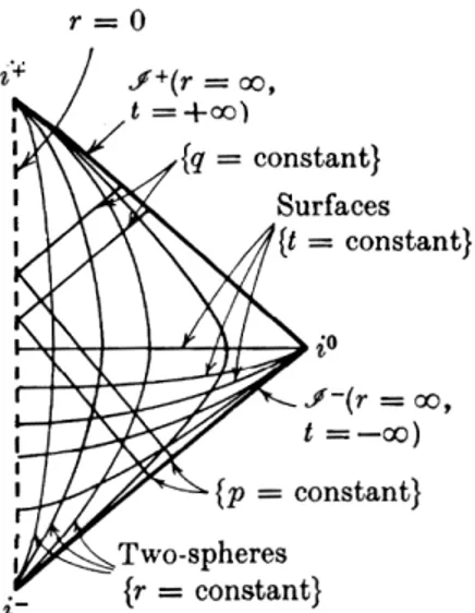
The aim of this chapter consists in introducing some fundamen-tal notions —both definitions and results— of pseudo-Riemannian geometry. We shall introduce the essential stuff that we shall need in the following chapters, above all to fix notations; for a definitely more complete treatment, we refer to [13] (in particular, Chap-ters III and V), [1], [18] (ChapChap-ters 0–4) and [19] (ChapChap-ters 1–4). Penrose diagrams, as well as notions about the Minkowski metric, are studied in [20] and [30].

In Section 2.1, we define differentiable manifolds and local co-ordinates, differentiability between two manifolds, tangent vec-tors and differentials. We also explain and assume the Einstein convention about repeated indices, a very useful notation tool in differential geometry.

Section 2.2 is dedicated to tensors and the tensor product. We also revise the exterior product and the exterior differentiation op-erator.

In Section 2.3, we review metric and pseudo-Riemannian man-ifolds. We also introduce the Laplace–Beltrami operator respect to a metric.

Section 2.4 is dedicated to the Minkowski metric. We use several coordinate systems to study this metric and represent it through a Penrose Diagram.

28 Differentiable manifolds §2.1

We conclude with Section 2.5, where we recall linear connec-tions and in particular Riemannian connecconnec-tions. These noconnec-tions lead to the definition of the Ricci tensor, which is the main char-acter of the Einstein equation, an important equation of general relativity that is the source of the topic of the following chapter and the setting of Chapters 4 and 5: the Schwarzschild metric.

2.1 Differentiable manifolds

An n-dimensional manifold is a Hausdorff topological space such that every point has a neighborhood homeomorphic to Rn_.

A chart (U, ϕ) of a manifold M is an open set U of M together with a homeo-morphism (a bijective bicontinuous application) ϕ : U → V onto a (necessarily) open set V ⊂ Rn_{. The coordinates (x}1_{, x}2_{, . . . , x}n_{) of the image ϕ(x) ∈ R}n_{of the}

point x ∈ U ⊂ M are called coordinates of x in the chart (U, ϕ); this is the reason why charts are also called local coordinate systems.

An atlas of class Ck_{on a manifold M is a set {(U}

α, ϕα)}α∈Asuch that:

• M =S_α∈AUα,

• the maps ϕβ ◦ ϕ−1α : ϕα(Uα∩ Uβ) → ϕβ(Uα∩ Uβ) are of class Ck.

Two Ck_{-atlases {(U}

α, ϕα)}α∈A and {(Uα, ϕα)}α∈A0 are equivalent if and only if

their union {(Uα, ϕα)}α∈A∪A0 is again a Ck-atlas.

A Ck_{-manifold is a manifold M together with a an equivalence class of C}k

-atlases. A smooth manifold is a C∞_{-manifold. If we require only the}

differ-entiability of the involved maps, we have differentiable atlases and

differen-tiable manifolds.

We use local charts to introduce the notion of differentiability on a manifold. Let us consider a real function defined on a manifold M, i.e. f : M → R. If (U, ϕ) is a chart at x, that is x ∈ U, then f ◦ ϕ−1 _{: ϕ(U) → R represents f in}

the local chart. We say that f is differentiable at x if, in a chart at x, f ◦ ϕ−1 _is

differentiable at ϕ(x). This is a suitable definition, since it does not depend on the choice of the chart. As a matter of fact, if f ◦ ϕ−1 _{is differentiable at ϕ(x),}

then f ◦ ϕ0−1_{is differentiable at ϕ}0_{(x) for every chart (U}0_{, ϕ}0_{) at x, since}

Ch. 2 ELEMENTS OFPSEUDO-RIEMANNIANGEOMETRY 29

More generally, given two differentiable manifolds M and N, we say that a function f : M → N is differentiable at x ∈ M if ψ ◦ f ◦ ϕ−1_{is differentiable at}

ϕ(x), where (U, ϕ) and (W, ψ) are local charts at x and at f (x) respectively.

The tangent vector space at a point can be defined following several ap-proaches. The straightest way is to say that a tangent vector vx to a smooth

manifold M at a point x is a linear map from the space of functions defined and differentiable on some neighborhood of x ∈ M into R that satisfies the Leibniz rule, i.e.

vx(af + bg) = avx(f ) + bvx(g) linearity,

vx(f g) = f (x)vx(g) + g(x)vx(f ) Leibniz rule

for all a, b ∈ R and for all real functions f, g on M differentiable at x. The space TxM of all such vectors, endowed with addition and scalar multiplication

defined by

(aux+ bvx)(f ) = aux(f ) + bvx(f ) ,

is a vector space called tangent vector space at the point x.

This definition of tangent vector can be made more precise through the no-tion of germ. We say that two funcno-tions on M differentiable at x have the same

germ at x if they coincide in a neighborhood of x. The equivalence class of

dif-ferentiable functions at x with the same germ of a function f is called germ of

f . Therefore, a tangent vector can be viewed as a derivation on the algebra of

germs of differentiable functions at x.

In the chart (U, ϕ), the local coordinates, or components, of a tangent vector are the set of numbers

vi = vx(ϕi) ,

where ϕi _{are the coordinates of ϕ in R}n_{. In the local chart (U, ϕ), if f is a C}1

-function on a neighborhood of x0 ∈ M, thanks to the mean value Lagrange

theorem we have, with ¯f = f ◦ ϕ−1_,

(2.1) f (x) = ¯f (ϕ(x0)) + (ϕi(x) − ϕi(x0)) ∂ ¯f ∂xi ¯ ¯ ¯ ¯ ϕ(x0)+s(ϕ(x)−ϕ(x0))

30 Differentiable manifolds §2.1

for some s ∈]0, 1[, where here and in the following we assume tacitly summation over repeated indices. More precisely, we adopt the Einstein convention about repeated indices: if the same index appears twice in the same formula, once up and once down, we suppose understood a sum over all the possible values for that index. For instance, formula (2.1) can be made explicit in the form

f (x) = ¯f (ϕ(x0)) + n X i=1 (ϕi_{(x) − ϕ}i_(x 0)) ∂ ¯f ∂xi ¯ ¯ ¯ ¯ ϕ(x0)+s(ϕ(x)−ϕ(x0)) .

At x0, the derivative of f along the vector vxis

(2.2) vx0(f ) = v i ∂ ¯f ∂xi ¯ ¯ ¯ ¯ ϕ(x0) , where vi _{= v} x0(ϕ i_{) .}

Each element vx∈ TxM can therefore be represented in the form

vx = vi

∂ ∂xi ,

where the vectors ∂/∂xi_{tacitly depend on x, according to (2.2). The set of these}

vectors, {∂/∂x1_{, ∂/∂x}2_{, . . . , ∂/∂x}n_{}, is a basis, called natural basis, for the}

tan-gent vector space, which has whence the same dimension of the manifold (note that the chart (U, ϕ) at x induces an isomorphism of TxM onto Rn ). The

el-ements of the dual basis of the natural basis, called natural cobasis, are often denoted by dxi_{, so that dx}i_(∂/∂xj_{) = δ}i

j, where the Kronecker δ symbol is

de-fined as δi j =    1 if i = j , 0 if i 6= j .

If f : M → N is a mapping differentiable at x between manifolds, we define the differential of f at x by

dfx : Tx(M) 3 v −→ w ∈ Tf (x)(N) ,

Ch. 2 ELEMENTS OFPSEUDO-RIEMANNIANGEOMETRY 31

w(h) = v(h ◦ f ) .

In the following, we shall simply write Txinstead of TxM.

2.2 Tensor and exterior products

M(V1, V2, . . . , Vn; W )

denote the (natural) vector space on K of all multilinear (i.e. linear in each component) maps from V1 × V2 × · · · × Vnto W . We assume that V1, V2, . . . , Vn

are finite-dimensional spaces, denote by V∗ _{the dual of a vector space V , and}

set

T = M(V₁∗, V₂∗, . . . , V_n∗; K) . If F ∈ M(V1, V2, . . . , Vn; T ) is given by

F (v1, v2, . . . , vn)(ϕ1, ϕ2, . . . , ϕn) = ϕ1(v1)ϕ2(v2) · · · ϕn(vn)

for all vi ∈ Vi and for all ϕi ∈ Vi∗, then we have the following result (see [1],

page 3, Theorem 1.1.3).

Theorem 2.2.1.With the notations above, we have that:

(a) for each vector spaceW onKand for eachΦ ∈ M(V1, V2, . . . , Vn; W ),there

exists a unique linear map Φ : T → W˜ such that Φ = ˜Φ ◦ F (universal

property of the tensorial product);

(b) if (T0_{, F}0_{) is another couple satisfying a), there exists a unique}

isomor-phismΨ : T → T0 _{such thatF}0 _{= Ψ ◦ F (uniqueness of the tensorial product).}

Two couples (T1, F1), (T2, F2), where Tj are vector spaces and

Fj ∈ M (V1, V2, . . . , Vn; Tj) ,

32 Tensor and exterior products §2.2

F2 = Ψ ◦ F1.

A couple (T, F ) satisfying the properties of Theorem 2.2.1(a) is called the

tensor product of the vector spaces V1, V2, . . . , Vnand denoted by V1⊗ V2⊗ · · · ⊗

Vn. Thanks to Theorem 2.2.1(b), the tensor product is well-defined modulo some

isomorphisms. The elements of the form F (v1, v2, . . . , vn) are denoted by v1 ⊗

v2⊗ · · · ⊗ vn.

In other words, if

vi ∈ Vi, ϕi ∈ Vi∗ i = 1, 2, . . . , n ,

we have

v1⊗ v2 ⊗ · · · ⊗ vn(ϕ1, ϕ2, . . . , ϕn) = ϕ1(v1)ϕ2(v2) · · · ϕn(vn)

and, from the multilinearity of F ,

λ(v1⊗ v2 ⊗ · · · ⊗ vn) = (λv1) ⊗ v2⊗ · · · ⊗ vn= · · · = v1⊗ v2⊗ · · · ⊗ (λvn) ,

v1⊗ · · · ⊗ (vi0+ vi00) ⊗ · · · ⊗ vn = v1⊗ · · · ⊗ vi0⊗ · · · ⊗ vn

+ v1⊗ · · · ⊗ vi00⊗ · · · ⊗ vn

for all λ ∈ K, for all v0

i, v00i ∈ Vi.

We introduce the following spaces:

T0 0(V ) = T0(V ) = T0(V ) = K , Tp(V ) = T0p(V ) = V ⊗ · · · ⊗ V_{| {z }} p times , Tq(V ) = Tq0(V ) = V_| ∗ ⊗ · · · ⊗ V_{{z }}∗ q times , T_qp(V ) = Tp(V ) ⊗ Tq(V ) . An element of Tp

q(V ) is called p-contravariant q-covariant tensor, or tensor of

type (p, q).

We denote by Sp the set of all permutations of (1, 2, . . . , p). It is known that

decompo-Ch. 2 ELEMENTS OFPSEUDO-RIEMANNIANGEOMETRY 33

sition can vary but the number of transpositions is always the same. We define the sign of a permutation σ, composition of r ∈ N transpositions, as

sign(σ) = (−1)r_.

Let V and W be two vector spaces over a field K of characteristics 0. A p-multilinear map ϕ : V × · · · × V → W is said to be an alternating map if

ϕ(vσ(1), vσ(2), . . . , vσ(p)) = sign(σ)ϕ(v1, v2, . . . , vp)

for every (v1, v2, . . . , vp) ∈ Vp and for every permutation σ ∈ Sp. We denote by

Λp_{(V ) the space of all p-covariant alternating tensors —which is hence a}

sub-space of Tp_{(V )— and, if the dimension of V is n, we set}

Λ(V ) = O

06p6n

Λp(V ) ;

note that Λ0_{(V ) = K.}

In order to define a product on this space, we introduce the operator

A :O p>0 Tp_{(V ) −→ Λ(V )} defined by A(α)(ϕ1_{, ϕ}2_{, . . . , ϕ}p_{) =} 1 p! X σ∈Sp sign(σ)α(ϕσ(1)_{, ϕ}σ(2)_{, . . . , ϕ}σ(p)₎

for every α ∈ Tp_{(V ) and ϕ}1_{, ϕ}2_{, . . . , ϕ}p _{∈ V}∗ _{(note that it is well-defined, linear}

and the identity on Λ(V )). Now, for each α ∈ Λp_{(V ) and β ∈ Λ}q_{(V ), we set}

α ∧ β = (p + q)!

p!q! A(α ⊗ β) ∈ Λ

p+q_{(V ) .}

Extending by bilinearity, we have the exterior product (or wedge product)

34 Pseudo-Riemannian manifolds §2.3

The quadruple (Λ(V ), +, ∧, ·) is an algebra called exterior algebra of V . Now, let M be a smooth manifold and α ∈ Λp_{(M) —that is, α}

x ∈ Λp(Tx)— be

of class Ck_{(in x). The exterior differentiation operator d maps α into dα ∈ Λ}p+1

of class Ck−1_{and satisfies the following conditions:}

(a) linearity: if λ is a constant,

d(α + β) = dα + dβ , d(λα) = λdα ;

(b) d(α ∧ β) = dα ∧ β + (−1)p_{α ∧ dβ ;}

(c) d2 _{= 0;}

(d) if f ∈ Ck_{(M), then df is the usual differential of f introduced in the}

previ-ous section.

These properties determine d uniquely, as shown in [13], page 200. Note that, if

f ∈ Ck_{(M), we set}

f α = f ∧ α

to simplify notations.

2.3 Pseudo-Riemannian manifolds

We call tensor field of order (p, q) a map that associates to each x ∈ M a tensor in Tp

q(Tx). For instance, a 2-covariant tensor field is a map

g : M 3 x −→ gx ∈ T2(Tx) .

A pseudo-Riemannian manifold is a couple (M, g), where M is a differen-tiable manifold and g is a differendifferen-tiable symmetric non-degenerate 2-covariant tensor field, called metric tensor or also pseudo-Riemannian metric. In other words, a pseudo-Riemannian metric provides a map M 3 x 7→ gx, where

gx : Tx× Tx → R is a bilinear map that satisfies:

• g is differentiable, that is, if (U, ϕ) is a chart at x, then gx(∂/∂xi, ∂/∂xj) is a

Ch. 2 ELEMENTS OFPSEUDO-RIEMANNIANGEOMETRY 35

• g is symmetric, that is,

gx(v, w) = gx(w, v) ∀v, w ∈ Tx, ∀x ∈ M ;

• for each x ∈ X, the bilinear form gxis non-degenerate, that is

gx(v, w) = 0 ∀w ∈ Tx if and only if v = Ox.

If we assume further that g is positive definite, i.e.

gx(v, v) > 0 ∀v ∈ Tx\ Ox, ∀x ∈ M

(so that each gx is a positive definite scalar product), we call it Riemannian

metric and say that (M, g) is a Riemannian manifold.

We denote by {e1, e2, . . . , en} a moving frame for the tangent space, that is,

for each x ∈ M, we have

ei

¯ ¯

x i = 1, 2, . . . , n

basis for Tx, while {ϑ1, ϑ2, . . . , ϑn} will be the dual basis. Hence, if we denote

the tensor g with ds2_{, we have}

g = ds2 _{= g} ijϑi⊗ ϑj = gijϑiϑj, where ϑi_ϑj ₌ 1 2 ¡ ϑi_{⊗ ϑ}j _{+ ϑ}j_{⊗ ϑ}i¢_,

because g is symmetric (remember that sum over repeated indices is assumed). Moreover, we have

gij = gx(ei, ej) ei, ej ∈ Tx

and an inner product on each vector space Tx defined by

36 Pseudo-Riemannian manifolds §2.3

An inner product on any vector space defines a canonical isomorphism be-tween the space and its dual. Indeed, for a fixed u ∈ Tx, the map

(u|·) : Tx 3 v −→ (u|v) ∈ R

is an element of T∗

x, hence the canonical isomorphism is given by

Tx 3 u −→ u∗ = (u|·) ∈ T. x∗.

Resorting to coordinates, we have (u|v) = gijuivj and hence u∗ = gijuiϑj. With

abuse of notation, one generally uses the same symbol u to indicate either u, either its image u∗_{. The u}i _{are called contravariant components of u, while}

ui are called covariant components of u; these components are related by the

formulae

ui = gijui, ui = gijuj,

where (gij_{) is the inverse of the matrix (g}

ij), i.e. gijgjk = δki. One says that indices

are raised or lowered by means of the tensor g. For instance, we have the mixed components:

ti_j = giktkj.

We have an inner product on T∗

x inducted by the canonical isomorphism, that is

(u∗_|v∗_{) = (u|v) = g}ik_u ivj,

and similar canonical isomorphisms, terminology and properties are used for tensors. In particular, all the following spaces are isomorphic:

Tp_(T

x) , Tp(Tx) , Tq(Tx) ⊗ Tp−q(Tx) .

Choosing a suitable basis {e0

i} for Tx, we can recast the expression for the

quadratic form gx(v, v) as a sum of k positive and n − k negative squares:

gx(v, v) = gijvivj = gij0 v0iv0j = k X i=1 (v0i₎2₋ n X i=k+1 (v0i₎2_.

Ch. 2 ELEMENTS OFPSEUDO-RIEMANNIANGEOMETRY 37

The number k does not depend on the choice of the basis and it is called index of the quadratic form, while the couple (k, n − k) is called signature. In terms of the basis {ϑ0i_{} dual to {e}0i_{}, we get}

gx = k X i=1 (ϑ0i)2− n X i=k+1 (ϑ0i)2.

A 4-dimensional pseudo-Riemannian manifold of index 1 is called

hyper-bolic manifold. As usual, we label with Greek indices the coordinates that take

the values 0, 1, 2, 3 and with Latin indices the ones that take the values 1, 2, 3. A basis {eα} on a hyperbolic manifold is called orthonormal if

(e0|e0) = 1 (ei|ei) = −1 , (eα|eβ) = 0

for all α 6= β. In terms of an orthonormal basis {ϑα_{}, one has}

g = (ϑ0)2− 3

X

i=1

(ϑi₎2_.

The (1 + n)-dimensional Minkowski space is the space R1+n_{with the metric}

(2.3) ds2 = (dx0)2−

n

X

i=1

(dxi)2

(of index 1), called Minkowski metric.

Given a metric g, represented by the matrix G = (gij), the Laplace–Beltrami

operator respect to g is the operator ∆g defined by

∆gf = p 1 | det G| ∂ ∂xi µ gijp| det G| ∂ ∂xjf ¶ , where f : M → K.

eu-38 Pseudo-Riemannian manifolds §2.3

clidean metric of signature (n, 0), i.e.

g =

n

X

i=1

(dxi₎2_,

the Laplace–Beltrami operator reduces to the standard Laplace operator ∆:

∆gf = ∆f = n X i=1 ∂2 if , ∂i = ∂ ∂xi .

When g is a metric of index 1, we write ¤g instead of ∆g, and we use the

symbol −∆gonly for the negative part of the metric. For instance, if we consider

the (1 + n)-dimensional Minkowski space, using the variables (t, x1, . . . , xn) ∈

R1+n_{, we have} ¤g = ∂t2− ∆g = ∂t2− ∆ = ∂t2− n X i=1 ∂2 i . = ¤ ;

hence, in this case, ¤g reduces to the standard d’Alembert operator ¤.

Example 2.3.1. R3_{with the euclidean metric g}

ij = δij induces on the sphere

S2 _{= {x ∈ R}3 _{: |x| = 1}}

the metric

(2.4) dω2 = dϑ2+ sin2 ϑdϕ2,

where we have chosen the parameters

(ϑ, ϕ) ∈]0, π[×]0, 2π[ so that, if x = (x1_{, x}2_{, x}3_{), we have}

(2.5) x1 _{= r sin ϑ cos ϕ , x}2 _{= r sin ϑ sin ϕ , x}3 _{= r cos ϑ .}