2020-07-09T12:47:48Z
Acceptance in OA@INAF
Anatomy of the AGN in NGC 5548. VIII. XMM-Newton's EPIC detailed view of an
unexpected variable multilayer absorber
Title
CAPPI, MASSIMO; De Marco, B.; PONTI, GABRIELE; Ursini, Francesco; Petrucci,
P. -O.; et al.
Authors
10.1051/0004-6361/201628464
DOI
http://hdl.handle.net/20.500.12386/26412
Handle
ASTRONOMY & ASTROPHYSICS
Journal
592
Number
DOI:10.1051/0004-6361/201628464 c ESO 2016
Astronomy
&
Astrophysics
Anatomy of the AGN in NGC 5548
VIII. XMM-Newton’s EPIC detailed view of an unexpected variable
multilayer absorber
M. Cappi
1, B. De Marco
2, G. Ponti
2, 1, F. Ursini
3, 4, P.-O. Petrucci
4, 5, S. Bianchi
3, J. S. Kaastra
6, 7, 8, G. A. Kriss
9, 10,
M. Mehdipour
6, 11, M. Whewell
11, N. Arav
12, E. Behar
13, R. Boissay
14, G. Branduardi-Raymont
11, E. Costantini
8,
J. Ebrero
15, L. Di Gesu
8, F. A. Harrison
16, S. Kaspi
13, G. Matt
3, S. Paltani
14, B. M. Peterson
17, 18,
K. C. Steenbrugge
19, and D. J. Walton
16, 201 INAF–IASF Bologna, via Gobetti 101, 40129 Bologna, Italy
e-mail: [email protected]
2 Max-Planck-Institut für extraterrestrische Physik, Giessenbachstrasse, 85748 Garching, Germany
3 Dipartimento di Matematica e Fisica, Università degli Studi Roma Tre, via della Vasca Navale 84, 00146 Roma, Italy 4 Université Grenoble Alpes, IPAG, 38000 Grenoble, France
5 CNRS, IPAG, 38000 Grenoble, France
6 SRON Netherlands Institute for Space Research, Sorbonnelaan 2, 3584 CA Utrecht, The Netherlands
7 Department of Physics and Astronomy, Universiteit Utrecht, PO Box 80000, 3508 TA Utrecht, The Netherlands 8 Leiden Observatory, Leiden University, PO Box 9513, 2300 RA Leiden, The Netherlands
9 Space Telescope Science Institute, 3700 San Martin Drive, Baltimore, MD 21218, USA
10 Department of Physics and Astronomy, The Johns Hopkins University, Baltimore, MD 21218, USA
11 Mullard Space Science Laboratory, University College London, Holmbury St. Mary, Dorking, Surrey, RH5 6NT, UK 12 Department of Physics, Virginia Tech, Blacksburg, VA 24061, USA
13 Department of Physics, Technion-Israel Institute of Technology, 32000 Haifa, Israel
14 Department of Astronomy, University of Geneva, 16 Chemin d’Ecogia, 1290 Versoix, Switzerland 15 European Space Astronomy Centre, PO Box 78, 28691 Villanueva de la Cañada, Madrid, Spain
16 Cahill Center for Astronomy and Astrophysics, California Institute of Technology, Pasadena, CA 91125, USA 17 Department of Astronomy, The Ohio State University, 140 W 18th Avenue, Columbus, OH 43210, USA
18 Center for Cosmology & AstroParticle Physics, The Ohio State University, 191 West Woodruff Ave., Columbus, OH 43210, USA 19 Instituto de Astronomía, Universidad Católica del Norte, Avenida Angamos 0610, 1280 Casilla, Antofagasta, Chile
20 Jet Propulsion Laboratory, California Institute of Technology, 4800 Oak Grove Drive, Pasadena, CA 91109, USA
Received 9 March 2016 / Accepted 5 April 2016
ABSTRACT
In 2013, we conducted a large multi-wavelength campaign on the archetypical Seyfert 1 galaxy NGC 5548. Unexpectedly, this usually unobscured source appeared strongly absorbed in the soft X-rays during the entire campaign, and signatures of new and strong outflows were present in the almost simultaneous UV HST/COS data. Here we carry out a comprehensive spectral analysis of all available XMM-Newton observations of NGC 5548 (precisely 14 observations from our campaign plus three from the archive, for a total of ∼763 ks) in combination with three simultaneous NuSTAR observations. We obtain a best-fit underlying continuum model composed by i) a weakly varying flat (Γ ∼ 1.5–1.7) power-law component; ii) a constant, cold reflection (FeK + continuum) component; iii) a soft excess, possibly owing to thermal Comptonization; and iv) a constant, ionized scattered emission-line dominated component. Our main findings are that, during the 2013 campaign, the first three of these components appear to be partially covered by a heavy and variable obscurer that is located along the line of sight (LOS), which is consistent with a multilayer of cold and mildly ionized gas. We characterize in detail the short timescale (mostly ∼ks-to-days) spectral variability of this new obscurer, and find it is mostly due to a combination of column density and covering factor variations, on top of intrinsic power-law (flux and slope) variations. In addition, our best-fit spectrum is left with several (but marginal) absorption features at rest-frame energies ∼6.7−6.9 keV and ∼8 keV, as well as a weak broad emission line feature redwards of the 6.4 keV emission line. These could indicate a more complex underlying model, e.g. a P-Cygni-type emission profile if we allow for a large velocity and wide-angle outflow. These findings are consistent with a picture where the obscurer represents the manifestation along the LOS of a multilayer of gas, which is also in multiphase, and which is likely outflowing at high speed, and simultaneously producing heavy obscuration and scattering in the X-rays, as well as broad absorption features in the UV.
Key words. galaxies: active – X-rays: galaxies – galaxies: individual: NGC 5548 1. Introduction
Unified models of active galactic nuclei (AGN) have ‘histori-cally’ been proposed as a static unifying view based on a puta-tive dusty molecular torus, where type 1 AGN are seen face-on,
thereby typically unabsorbed and bright, while type 2 sources are seen edge-on, thus typically obscured and faint (Antonucci & Miller1985). However in recent years, an ever increasing num-ber of type 1 Seyfert galaxies/AGN (up to 20−30% of limited samples) have shown a significant amount of absorption that is
clearly at odds with the source’s optical classifications (Bassani et al.1999; Cappi et al.2006; Panessa et al. 2009; Merloni et al. 2014). Such complex, often variable, absorbing structures seem to call for a revision of the static version of unified models into a more complex, maybe dynamical, structure (e.g. Murray et al. 1995; Elvis2000; Proga2007).
On the one hand, ionized absorbers (so-called warm ab-sorbers, WA) are nowadays routinely observed as blue-shifted, narrow, and broadened absorption lines in the UV and X-ray spectra of a substantial (certainly greater than 30%) fraction of AGN and quasars (e.g. Blustin et al.2005; Piconcelli et al.2005; McKernan et al.2007; Ganguly & Brotherton2008). These ab-sorption systems span a wide range of velocities and physical conditions (distance, density, ionization state), and may have their origin in an AGN-driven wind, sweeping up the interstellar medium, or thermally driven from the molecular torus (Blustin et al.2005) and outflowing at hundreds to few thousands km s−1 (see Crenshaw et al.2003aand Costantini2010for reviews on the subject). Even more powerful outflows (the so-called ul-tra fast outflows, UFOs), which are so highly ionized that their only bound transitions left are for Hydrogen- and Helium-like iron, detectable only at X-ray energies, seem to be present in 30−40% of local radio-quiet and radio-loud AGN, with out-flow speeds of up to ∼0.3c (Pounds et al.2003a; Tombesi et al. 2010,2013,2014; Gofford et al.2013). Both WA and UFO phe-nomena have been seen to vary on both short (hours-days) and long (months-years) time-scales (Cappi2006) for various plausi-ble reasons, such as variations in either the photoionization bal-ance, or the absorption column density and/or covering fraction (Risaliti et al.2005; Reeves et al.2014).
On the other hand, there is also mounting evidence for the presence of large columns of additional neutral or mildly ionized gas along the LOS to not only type 2 Seyfert galaxies (e.g. Turner et al. 1997, 1998) but also type 1 and intermediate Seyferts (e.g., Malizia et al.1997; Pounds et al.2004; Miller et al.2007; Bianchi et al.2009; Turner et al.2009; Risaliti et al.2010; Lob-ban et al. 2011; Marchese et al.2012; Longinotti et al.2009, 2013; Reeves et al. 2013; Walton et al. 2014; Miniutti et al. 2014; Rivers et al. 2015). In some cases, the columns are so large that astronomers have called these “changing look” sources (i.e. sources changing from being absorbed by a Compton thin to a Compton thick column density). From the pioneering works of Risaliti et al. (Risaliti et al. 2002,2005) on a few interest-ing sources such as the Seyfert 1 NGC 1365, to detailed studies on an increasing number of sources and on systematic studies of larger samples (Markowitz et al. 2014; Torricelli-Ciamponi et al. 2014; Tatum et al.2013), evidence has accumulated for the importance of large, complex, and variable neutral absorp-tion also in type 1 Seyfert galaxies. Current interpretaabsorp-tions for this cold circumnuclear gas are clumpy molecular tori (Krolik & Begelman1988, Markowitz et al.2014; Hönig 2013), absorp-tion from inner and/or outer BLR clouds (Risaliti et al.2009), or accretion disc outflows (Elitzur & Shlosman2006; Proga2007; Sim et al.2008).
NGC 5548 (z = 0.017) is one of the X-ray brightest (2– 10 keV flux of ∼2–5 × 10⁻¹¹ erg cm−2s−1), and most luminous (L2−10 keV ∼ 1−3 × 1044 erg/s) Seyfert 1 galaxies known. As
such, it is one of the best-studied example of a Seyfert 1 galaxy and has been observed by all major satellites since it entered the Ariel V high galactic latitude source catalog (Cooke et al. 1978). NGC 5548 exhibits all the typical components seen in type 1 Seyfert galaxies, that is: a steep (Γ ∼ 1.8–1.9) power-law spectrum plus a reflection component with associated FeK line, a soft-excess emerging below a few keV, evidence for warm
ionized gas along the LOS, and typical soft X-ray variability, as shown in the CAIXAvar sample by Ponti et al. (2012a). Re-cently, detailed studies of either the time-average or variability properties of the WA, the reflection component, and the soft-excess component have been made using either low- (CCD-type) or higher-(grating-type) energy resolution instrumentation avail-able from Chandra, XMM-Newton and Suzaku (Pounds et al. 2003a,b; Steenbrugge et al.2003,2005; Crenshaw et al.2003a,b; Andrade-Velazquez et al.2010; Krongold et al.2010; Liu et al. 2010; Brenneman et al.2012; McHardy et al.2014).
In 2013, our team conducted a long multi-satellite observing campaign on NGC 5548. The campaign is introduced in detail in Mehdipour et al. (2015; hereafter Paper I). The main results from the campaign, the simultaneous appearance of an excep-tional obscuring event in the X-rays and a broad absorption line (BAL) structure in the UV, are presented in Kaastra et al. (2014; hereafter Paper 0). The shadowing effects of this UV BAL and X-ray obscurer on the larger-scale “historical” UV narrow ab-sorption lines and WA are presented in Arav et al. (2015; here-after Paper II). The high energy properties of the source during, and before, the campaign are shown in Ursini et al. (2015; here-after Paper III), while the study of a short-timescale flaring event that happened in September 2013 and which triggered a Chan-draLETG observation is addressed in Di Gesu et al. (2015; here-after Paper IV), together with the analysis of the WA short-term variability during this event. The time-averaged soft X-ray line-dominated RGS spectrum is presented and modeled in detail in Whewell et al. (2015; hereafter Paper V). For the longer-term timescales, the historical source behavior is presented in Ebrero et al. (2016a,b; hereafter Paper VI), while the full Swift multi-year monitoring is presented in Mehdipour et al. (2016; hereafter Paper VII).
Here, we focus on the detailed model characterization of the obscurer, and of its spectral variability, by making use of all available EPIC (pn+MOS) spectra (during and before the campaign) and simultaneous NuSTAR observations (Sect. 2). We also incorporate in our modeling the results from the pa-pers mentioned above, which were obtained during the cam-paign and which were based on other instruments and satellites, such as RGS spectra, HST/COS spectra, and Swift long-term light-curves. This allows us to draw a comprehensive and self-consistent understanding of the obscurer properties (Sect. 4). We then attempt to place constraints on the location and physical ori-gin of the various components required by our model (Sect. 5). Values of H0 = 70 km s−1 Mpc−1, and ΩΛ = 0.73 are
as-sumed throughout, and errors are quoted at the 90% confidence (∆χ2= 2.71) for 1 parameter of interest, unless otherwise stated.
2. Observations and data reduction
NGC 5548 was observed by the XMM-Newton EPIC instruments on 17 separate occasions, for a total cleaned exposure time of ∼763 ks (see Table 1). The first three (archival) observations were performed once in December 2000 and twice in July 2001. The remaining 14 observations were all part of the 2013 mul-tiwavelength campaign (Paper 0 and Paper I). Twelve observa-tions were performed during the summer 2013, one five months later, in December 2013, and the last one in February 2014. The spacing was intentional to sample different timescales in a rough logarithmic spacing, i.e. multiple on short (days) timescales, and more sparse on longer (months) timescales. A full description of the numerous observations performed during the campaign, from space and ground observatories, is given in Paper I.
Table 1. Summary of NGC 5548 XMM-Newton (pn) and NuSTAR observations.
Obs. Obs. ID Start-End datea Exposureb F
(0.5−2)c F(2−10)d F(10−30)e Archival data (2000–2001) A1 0109960101 2000 Dec. 24–25 16.1 17.2 32.8 – A2 0089960301 2001 Jul. 09–10 56.7 20.9 40.3 – A3 0089960401 2001 Jul. 12–12 18.9 28.7 50.8 – Multiwavelength campaign (2013) M1 0720110301 2013 Jun. 22–22 35.4 1.14 15.3 – M2 0720110401 2013 Jun. 30–30 38.1 3.59 33.0 – M3 0720110501 2013 Jul. 07–08 38.9 2.16 23.9 – M4N 0720110601 2013 Jul. 11–12 37.4 3.66 35.8 – . . . 60002044002/3∗ 2013 Jul. 11–12 51.4 3.66 35.8 51.0 M5 0720110701 2013 Jul. 15–16 37.5 2.62 29.9 – M6 0720110801 2013 Jul. 19–20 37.1 2.38 30.5 – M7 0720110901 2013 Jul. 21–22 38.9 2.28 26.3 – M8N 0720111001 2013 Jul. 23–24 37.5 2.21 27.9 – . . . 60002044005∗ 2013 Jul. 23–24 49.5 2.21 27.9 45.0 M9 0720111101 2013 Jul. 25–26 32.1 3.14 33.2 – M10 0720111201 2013 Jul. 27–28 38.9 3.01 32.4 – M11 0720111301 2013 Jul. 29–30 35.3 2.76 29.6 – M12 0720111401 2013 Jul. 31–Aug 01 36.1 2.28 26.2 42.8 M13N 0720111501 2013 Dec. 20–21 38.2 2.08 24.9 – . . . 60002044008∗ 2013 Dec. 20–21 50.1 2.08 24.9 – M14 0720111601 2014 Feb. 04–05 38.8 3.96 27.2 –
Notes.(a)Observation start-end dates.(b)Net exposure time, after corrections for screening and deadtime, in ks.(c)Observed flux in the 0.5–2 keV
band, in units of 10−12erg cm−2s−1.(d)Observed flux in the 2–10 keV band, in units of 10−12erg cm−2s−1.(e)Observed flux in the 10–30 keV
band, in units of 10−12erg cm−2s−1.(∗)NuSTARobservations simultaneous to the XMM-Newton observations.
The EPIC data were reduced using the standard software SAS v. 14 (de la Calle2014) and the analysis was carried out using the HEASoft v. 6.14 package1.
After filtering for times of high background rate, and correc-tion for the live time fraccorrec-tion (up to 0.7 for the pn in small win-dow mode), the useful exposure times were typically between 30 and 50 ks per observation (see Table1). The EPIC pn and MOS cameras were operated in the so-called small window mode with the thin filter applied for all observations, except for the first three archival observations (A1-3) for which the MOS 1 cam-era was opcam-erated in timing mode, thus the MOS1 was not used for this analysis.
Using the epatplot command of the SAS, we checked the pattern distributions of the collected events and found that: (i) pile-up was not significant (less than few %) in the pn data at this level of source flux (and notably during the campaign when the source was heavily absorbed), thus we considered both single and double events as per standard procedure and cali-brations; (ii) the pattern distribution in the pn deviates signif-icantly below 0.4 keV with respect to model predictions, thus we did not consider the data below 0.4 keV in the present anal-ysis. We note that this is slightly different from our previous analysis reported in Papers 0, III, and IV, in which we always used data down to 0.3 keV. We estimate that the effect of this slightly different choice of low-energy cut-off should neverthe-less be largely within statistical errors of the present and previous analysis. Given the significantly lower effective area of the MOS detectors, and for clarity and simplicity, we only report here the results obtained from the pn data and used the MOS data only for consistency checks.
Source counts were extracted from a circular region of 40 arcsec radius, while the background counts were extracted from a nearby source-free and gap-free area of the detector of
1 http://heasarc.gsfc.nasa.gov/docs/software/lheasoft/
the same size. The size of the small window being less than 4.50×4.50, both source and background were similarly affected by the instrumental Ni and Cu Kα lines at 7.3−7.6 keV and 7.8−8.2 keV, respectively, thereby cancelling out their effects.
Finally, we anticipate that all the Fe K line measurements (see Sect. 4.1.2 below) obtained with the pn spectra during the campaign, but not in the earlier archival data, presented a sys-tematic (and more or less constant) blueshift and broadening of the energy scale response by ∆E ∼ +30–40 eV and σ(E) ∼ 40– 50 eV, respectively, when compared to the MOS and/or NuSTAR independent results. These shifts, albeit being modest, were nev-ertheless statistically significant and present with either single and double or single-only events, and despite our use of the lat-est CTI correction files (CCFv45, released in November 2014) and analysis procedure, as described in Smith et al. (2014). To investigate this further, we performed a detailed analysis of the spectral energy scale by comparing our results for different in-struments (MOS1, MOS2, pn, and NuSTAR), using different pat-tern selections (from single-only to single+double events), and applying different CTI response correction files (from CCF v27 to v45) which were released in 2013 and 2014. We also com-pared our results with the energy and width obtained for the AlK line (at 1486 eV) and the MnK doublet (at 5895 and 6489 eV) of the calibration source during a ∼70 ks CALCLOSED observa-tion performed in 2013, August 31st, i.e. shortly after the cam-paign and thus representative of the absolute energy scale of the instrument at that time. From this analysis, we attributed both blueshift and broadening to a remaining (admittedly small) un-certainty in the long-term degradation of the EPIC pn CTI, as mentioned in the calibration technical notes of Guainazzi et al. (2014) and Smith et al. (2014). In the following analysis, we thus took into account these systematic shifts and broadenings by us-ing the zashift and gsmooth command in XSPEC to correct for this remaining uncertainty (see also Sect. 4.1.2).
1
10
S(0.4−2 keV)
A1 A2 A3 M1 M2 M3 M4N M5 M6 M9 M10 M11 M121
2
5
H(2−10 keV)
M7 M8N M13N M140
2×10
54×10
56×10
58×10
51
0.2
0.5
2
H/S
Time (s)
Fig. 1.Background subtracted XMM-Newton pn light curves of NGC 5548 calculated for the soft (S) 0.4−2 keV energy band (top), the hard (H)
2−10 keV energy band (middle) and their hardness ratios H/S (bottom). Vertical dashed lines indicate when observations were interrupted during the years.
We also used data from three (out of 4) NuSTAR observa-tions, those which were simultaneous to the XMM-Newton ob-servations, namely the 4th, 8th and 13th observations of the XMM-Newton campaign (see Table 1). A comprehensive anal-ysis of the high-energy continuum, combining all available NuSTAR, INTEGRAL, and previous BeppoSAX and Suzaku ob-servations is presented in Paper III. We followed their same pro-cedure for the NuSTAR data reduction, i.e. we used the standard pipeline (nupipeline) of the NuSTAR Data Analysis Software (nustardas, v1.3.1; part of the heasoft distribution as of ver-sion 6.14) to reduce the data, and used the calibration files from the NuSTAR caldb v20130710. The spectra were then extracted from the cleaned event files using the standard tool nuproducts for each of the two hard X-ray telescopes aboard NuSTAR, which have corresponding focal plane modules A and B (FPMA and FPMB). The spectra from FPMA and FPMB were analyzed jointly, but were not combined. Finally, the spectra were grouped such that each spectral bin contains at least 50 counts.
3. Timing analysis
Soft (0.4−2 keV) and hard (2−10 keV) band light curves of NGC 5548 are shown in Fig. 1 (top and middle panels, re-spectively) with a time bin of 2000 s. Hardness ratios (bottom panel) are also reported to highlight any spectral variations of the source. The light curves include the three archival (year 2000−2001) observations, and the 14 observations of the mul-tifrequency campaign (year 2013−2014), with each observation separated by vertical dotted lines. Within the single observa-tions (including time scales of <few tens of ks) we observe only low/moderate flux variations (less than 20−30 percent of the av-erage flux). However, much stronger flux variations (>50 per-cent) occur between the different observations, on the time scales sampled by the campaign and longer (i.e. up to years, if we also consider the three archival XMM-Newton observations).
As already presented in Papers 0 and I, the hardness ra-tios show a significant spectral hardening which characterizes the 2013−2014 campaign, when compared to the 2000−2001 archival data. The source does not show any significant spec-tral variation within each (∼half a day long) observation, besides a hint of spectral softening during the last observation. The lack of significant short-term spectral variability justifies our spectral analysis approach below (Sect. 4) of averaging the spectra ob-servation by obob-servation.
To better characterize the distribution of variability power as a function of energy band, we computed the fractional root mean squared (rms) variability amplitude (Fvar; Nandra et al. 1997;
Vaughan et al.2003; Ponti et al.2004; Ponti2007) on both short (hours) and long (days-to-months) timescales. The former is ob-tained by extracting light curves of the single pn observations, with a time bin of 2 ks, and averaging the Fvar computed from
each of them. The latter is obtained by taking the average count rates of each observation and computing the Fvarover the entire
campaign, thus sampling timescales going from ∼45 ks up to 20 Ms. The light curves are extracted in different energy chan-nels, the width of the channels ensuring the number of counts 20 per time and energy bin. Results are shown in Fig.2. The Fvarshows, in a clear and model-independent way, that the peak
of variability power (∼30 percent) lies in the energy band be-tween 1 and 5 keV, and most of the variability occurs on the long timescales. This shape is very similar to what is typically observed also in other Seyfert galaxies (Ponti2007). Remark-ably, a narrow feature is very clearly observed here at the energy of the Fe Kα line, which strongly suggests the presence of a con-stant (on long timescales) reflection component.
It is worth noting that, despite being very low (few percents), the Fvar of the short timescales is significantly different from
zero. We verified that this residual variability is most likely to be ascribed to red-noise leakage effects (e.g. Uttley et al.2002), rather than to intrinsic, short-term variability of the source. In other words, variability over timescales slightly longer than the
1 10 0.5 2 5 0 0.1 0.2 0.3 Fvar Energy (keV) 2 ks < Short T < 25 ks 45 ks < Long T < 20 Ms
Fig. 2.Fractional variability (rms) spectra of NGC 5548 calculated over
long (45−2000 ks, top curve) timescales, i.e. longer than observations durations, but shorter than overall campaign, and over short (2−25 ks, bottom curve) timescales, i.e. longer than minimum time bin but shorter than shortest observation duration.
maximum sampled timescale (limited by the duration of the ob-servation) has introduced slow rising and falling trends across the light curve of the single observations, which have contributed to its short-timescale variance. As a consequence, variability power from long timescales has been transferred to the short timescales. Variability studies on even longer timescales than those presented here (using Swift light curves) are presented in McHardy et al. (2014) and Paper VII.
4. Spectral analysis
Within each observation, the source varied only very weakly ei-ther in flux (top and medium panels of Fig. 1) or in spectral shape (bottom panel of Fig.1), as found also from the very low Fvarvalue when calculated on short-timescales (Fig.2). We thus
extracted the mean pn spectra for each of the 17 observations, grouping the data to a maximum of 10 channels per energy res-olution element and 30 counts per channel to apply the χ2
mini-mization statistics. In all following fits, the Galactic column den-sity was fixed at the value of NHgal = 1.55 × 1020cm−2(Dickey
& Lockman 1990), and abundances were taken from Lodders (2003).
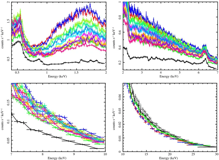
Figure3shows the overall XMM-Newton spectra during all observations (1−17) which clearly show the strong absorption that is affecting all the 0.3−10 keV spectra during the 2013 cam-paign (obs. 4−17, in color) when compared to the 2000−2001 archival unabsorbed spectra (obs. 1−3, in black). Figure4 fur-ther illustrates the complex and strongly energy-dependent vari-ability of the source during the campaign: the top two panels show the large and complex variability in the soft 0.4−2 keV (top left panel) and hard 2−7 keV (top right panel). The two bot-tom panels show the reduction in variability going from lower (7−10 keV) to higher (10−30 keV) energies. Because of the heavy and variable absorption affecting the source, the spectrum is very complex and model parameters (such as the photon in-dex Γ, the absorption column densities, and their covering fac-tors) are often strongly degenerate. Moreover, during the unob-scured, archival observations (A1→3) the source shows a very
significant, moderately strong, soft-excess (see e.g. Pounds et al. 2003b) which is however not easy to detect during the monitor-ing campaign (M1→14) because of the heavy obscuration.
To overcome, or minimize, the above limitations we de-cided to proceed in the following way: first, we used the three XMM-Newton spectra for which NuSTAR was simultaneously available, and used data at first only above 4 keV, to obtain the best possible constraints on the underlying source continuum components, in particular the reflection component. Second, we considered also the data below 4 keV, using all information from previous papers in this series and from literature, and also com-bine the information at soft X-rays obtained from the archival XMM-Newtonobservations. These two different steps and stud-ies (Sects. 4.1 and 4.2) are preliminary and crucial to then best characterize the obscurer variability using the whole dataset of XMM-Newtonobservations.
4.1. Hard (>4 keV) X-ray band: underlying continuum and constant reflection component
4.1.1. The three XMM-Newton+NuSTAR simultaneous observations
As mentioned above, we first considered only the data in the 4– 79 keV interval where the data are less sensitive to the precise modeling of the obscurer, in an attempt to minimize degenera-cies induced by the absorbers. XMM-Newton and NuSTAR spec-tra were fitted individually for each of the three simultaneous observations, with the same model, but letting all parameters free to vary, except for the normalizations of the two NuSTAR modules (FPMA/B), which were kept tied together. For plotting purposes only, and to better identify any systematic deviation from the fits, the spectra were then grouped together (using the setplot group command in XSPEC) and color-coded with pn spectra in black and NuSTAR spectra in red. Cross-normalization values among different instruments (FPMA vs. FPMB vs. pn) were always left free to vary but these were never larger than a few percent, typically 2−3%, in line with expectations (Madsen et al.2015).
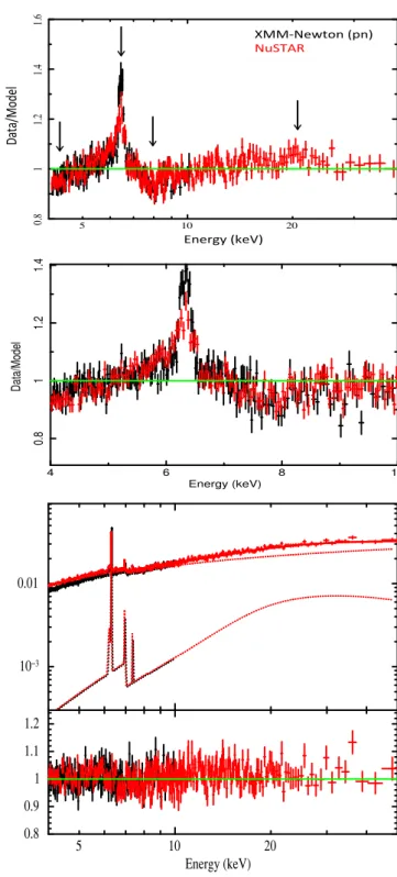
Figure 5 shows the ratios (between ∼4−50 keV) obtained from a fit of the 4−79 keV spectra with a single non-absorbed power-law model (with Γ ∼ 1.3−1.5). Low energy curvature, a narrow line at ∼6.4 keV and a high energy hump between 10−30 keV are readily seen in the data (see Fig.5, top). We thus added a cold absorption column density plus a Gaussian emis-sion line and a continuum reflection model (pexrav in XSPEC). Despite the possible presence of additional absorption feature(s) between 7−8 keV (see Fig. 5, bottom panel, and following anal-ysis in Sect. 4.5), the use of a more complex absorber, either partially covering or ionized, was not required here when fitting the continuum above 4 keV, likely because of the strongly curved low-energy cut-off which requires a substantially cold absorber to be modeled, with NH' 4–7 × 1022cm−2(Table2).
Best-fit parameters obtained from XMM-Newton only were in very good agreement (typically within a 1-σ error) with those obtained with NuSTAR only, except for a mildly flatter slope (by ∆Γ ∼ 0.1) required for XMM-Newton with regard to NuSTAR. Within each observation, we choose to tie all parameters ob-tained from both instruments, except for letting their cross-normalizations and photon index free to vary (to take into ac-count the remaining calibration uncertainties), but report here and below values of photon indices and fluxes obtained for the pn only to allow better comparison with observations with-out the NuSTAR simultaneous data. Best-fit values for the three
1 10 0.5 2 5
0.01
0.1
1
10
counts s
1keV
1 Energy (keV) Archival Observa.ons 1) 24/12/2000 2) 09/07/2001 3) 12/07/2001New Monitoring Campaign
4) 22/06/2013 11) 23/07/2013 5) 30/06/2013 12) 25/07/2013 6) 07/07/2013 13) 27/07/2013 7) 11/07/2013 14) 29/07/2013 8) 15/07/2013 15) 31/07/2013 9) 19/07/2013 16) 20/12/2013 10) 21/07/2013 17) 04/02/2014
Fig. 3.The 0.4−10 keV spectra of NGC 5548 obtained with the EPIC pn during the three archival observations (black) and during the 14
observa-tions of the 2013 summer campaign (color). Observaobserva-tions are summarized in Table 1.
0.5 1 1.5 2 0.5 1 1.5 2 counts s −1 keV −1 Energy (keV) 2 3 4 5 6 7 0.2 0.4 0.6 0.8 1 counts s −1 keV −1 Energy (keV) 7 8 9 10 0.05 0.1 0.15 counts s −1 keV −1 Energy (keV) 10 15 20 25 30 0 0.01 0.02 0.03 0.04 counts s −1 keV −1 Energy (keV)
Fig. 4.X-ray spectra obtained during the campaign (M1→M14, including the simultaneous M4N, M8N and M13N NuSTAR observations plotted
above 10 keV) plotted on linear scales, and with the same factor of ∼10 extension range (from bottom to top) in the y-axis scale intensities. These are shown to illustrate the important and complex variability as a function of energy up to 2 keV, and its gradual reduction above 2 keV, and up to 30 keV.
10 5 20 0.8 1 1.2 1.4 1.6 ratio Energy (keV) XMM-‐Newton (pn) NuSTAR Data/ Mo de l Energy (keV) 4 6 8 10 0.8 1 1.2 1.4 Data/Model Energy (keV) 10−3 0.01 keV 2 (Photons cm −2 s −1 keV −1 ) 10 5 20 0.8 0.9 1 1.1 1.2 Ratio Energy (keV)
Fig. 5.Top: data are plotted as the ratio to a single power-law
contin-uum model fitted to the grouped observations M4N, M8N, and M13N with XMM-Newton (black) and NuSTAR (red) simultaneous data. As in-dicated by the arrows, going from low to high energies, one can clearly note the presence of: a sharp low-energy cut-off, a narrow Fe K line at ∼6.4 keV, some absorption feature(s) between 7−8 keV, and a high en-ergy hump between 10−30 keV. Middle: same as top panel, but zoomed between 4 and 10 keV. Bottom: best-fit spectrum, model, and ratios plot-ted between 4−50 keV (see Sect. 4.1.1 for details).
observations are reported in Table2. These values are consistent with those obtained by Papers III and IV.
Given the neutral energy for the Fe K line, its nar-row width, and its constant intensity, the line is consistent with being produced by reflection from a cold and distant
reflector (see Sect. 5.1 for further discussion). This is consis-tent with our analysis below (Sect. 4.1.2) using the whole set of XMM-Newton observations. This agrees also with our pre-vious (model-independent) findings based on the source frac-tional variability amplitude (Sect. 3). The line equivalent width (EW ∼ 70–110 eV) with respect to the underlying continuum re-flection (R ∼ 0.56–0.91, see Table2) is consistent with the line being produced by a plane parallel neutral Compton thick re-flector, and solar abundance, thus we decide to choose, for sim-plicity, the XSPEC model pexmon (Nandra et al. 2007), which gives a self-consistent description of both the neutral Fe Kα
line and the Compton reflection continuum. This model also self-consistently generates the Fe Kβ, Ni Kα, and Fe Kα
Comp-ton shoulder expected from a CompComp-ton-thick reflecting medium. Following the results presented in Paper III, we assumed, and fixed, the parameters of the intrinsic continuum illuminating the reflection slab to typical values of Γ = 1.9, Ec = 300 keV,
in-clination =30 deg, and solar abundances. With this model, we obtained the best-fit parameters listed in Table2. These values are in agreement with those shown in Paper III.
From now on, in this analysis these values will be referred to as our baseline underlying continuum model. Moreover, mo-tivated by the fact that the line intensity did not vary significantly (neither in intensity nor in energy) during the other 14 available observations (see Sect. 4.1.2), we decided to freeze the reflec-tion component to the average value obtained from the three XMM-Newton+ NuSTAR simultaneous observations, i.e. a nor-malization at 1 keV of 5.7 × 10⁻³photons keV−1cm−2s−1, also in agreement with Paper III.
4.1.2. The whole 17 XMM-Newton observations
Given the above results, we thus proceeded in our analysis by adding to the previous observations (M4N, M8N, and M13N) the other 14 available XMM-Newton observations, including the three archival observations and the remaining 11 from the 2013 campaign. Again, the spectra were first considered only above 4 keV and focusing on the properties of the Fe K line and reflec-tion component before and during the campaign.
Following the previous analysis, we first fitted all the 17 XMM-Newton spectra with a single, cold, absorber plus an Fe Kα line, plus a pexrav continuum reflection model. This sim-ple model yielded a good characterization of all XMM-Newton spectra, as demonstrated by the grouped spectrum shown in Fig.6. The time-series for the Fe K line parameters during all 17 observations are shown in Fig.7. We note that the line energy during the campaign was slightly higher ('6.43 ± 0.01 keV) than during the first three archival observations ('6.39 ± 0.01 keV), and was also systematically higher than the energy '6.40 ± 0.01 keV obtained using only the MOS data. As discussed in Sect. 2, we attribute the energy shift, and slight broadening, of the FeK line to remaining CTI response degradation that has not properly been accounted for.
The line is consistent with being constant in intensity during all the 17 observations (Fig.7, bottom panel), i.e. not only dur-ing the campaign, but also after comparison with the (∼13 years) earlier archival observations. Overall, in agreement with our earlier findings, which are based on the fractional variability (Sect. 3), this analysis readily demonstrates that the Fe K line emission is neutral, narrow and, most importantly, constant in time. We thus choose again to model both line and continuum using the self-consistent cold reflection model pexmon, and fit all data with the reflection intensity fixed at its average value (5.7 × 10⁻³photons keV−1cm−2s−1) obtained in Sect. 4.1.1, and
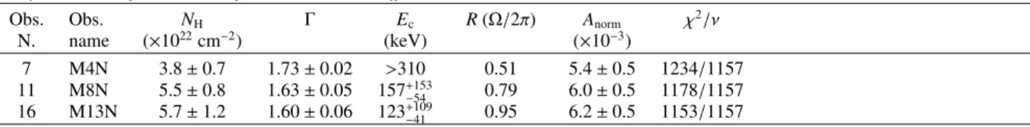
Table 2. Hard (4–79 keV) X-ray continuum emission (XMM-Newton +NuSTAR observations): Power law plus reflection models. Phenomenological reflection model (cut-off-PL + Fe Kαemission line+ pexrav)
Obs. Obs. NH Γ Ec Energy1 EW2 Int.3 R(Ω/2π) Anorm χ2/ν
N. name (×1022cm−2) (keV) (keV) (eV) (×10−5) (×10−3)
7 M4N 4.1 ± 0.5 1.74 ± 0.04 >313 6.35 ± 0.02 69 ± 9 3.0 0.56 5.9+0.9 −1.3 3535/3471 11 M8N 7.2+0.5 −1.0 1.75 ± 0.06 >212 6.38 ± 0.02 83 ± 10 3.0 0.65 6.2 +1.1 −1.4 3535/3471 16 M13N 5.8+0.6 −1.2 1.60 ± 0.04 129 +48 −30 6.42 ± 0.02 110 ± 10 3.7 0.91 5.9 +1.0 −0.5 3535/3471
Physical and self-consistent reflection model (cut-off-PL + pexmon)
Obs. Obs. NH Γ Ec R(Ω/2π) Anorm χ2/ν
N. name (×1022cm−2) (keV) (×10−3) 7 M4N 3.8 ± 0.7 1.73 ± 0.02 >310 0.51 5.4 ± 0.5 1234/1157 11 M8N 5.5 ± 0.8 1.63 ± 0.05 157+153 −54 0.79 6.0 ± 0.5 1178/1157 16 M13N 5.7 ± 1.2 1.60 ± 0.06 123+109 −41 0.95 6.2 ± 0.5 1153/1157
Notes.(1)Emission line rest-frame energy centroid, in units of keV.(2)Emission line rest-frame equivalent width in units of eV. The width of the
line was fixed to σ = 0.1 keV (see text for details).(3)2–10 keV flux in units of 10−11erg s−1cm−2.
0.01 5×10⁻³ 0.02 keV 2 (Photons cm −2 s −1 keV −1 ) 4 6 8 10 0.95 1 1.05 Ratio Energy (keV)
Fig. 6.The 4−10 keV band spectrum obtained from the individual fitting
of all the 17 XMM-Newton spectra, and the data/model ratios, grouped in a single dataset.
then freezing the zashift parameter to its best-fit value. We note that this simple analysis readily shows that, during the cam-paign, the photon index was flatter (Γ ∼ 1.5–1.7) than typically found during either the three archival observations or historically in this source (Γ ∼ 1.7–1.9, e.g. Dadina2007), and despite al-lowing in the fit for large absorption column densities with val-ues between log NH∼ 22–23 cm−2.
4.2. Soft (<4 keV) X-ray band: warm absorber, intrinsic soft-excess and scattered component
As mentioned above, the soft (E < 4 keV) X-ray spectrum of this source is known to be rather complex. Historically, it is known to require at least two components to be properly modeled, such as a complex, multi-temperature warm absorber, plus an intrinsic soft X-ray emission component (commonly called soft-excess). In this part of the spectrum, we require at least one additional component, a soft scattered component, to be consistent with
6.35 6.4 6.45
A1 A2 A3 M1 M2 M3 M4N M5 M6 M7N M8 M9 M10 M11 M12 M13N M14
Rest Energy (keV)
0 0.02 0.04 0.06 0.08 Line Width σ (keV) 5 10 15 2×10⁻⁵ 3×10⁻⁵ 4×10⁻⁵ Observation Number Line Intensity
Fig. 7.Time series of the FeK line best-fit parameters: Rest-frame
en-ergy (top, black) in keV, line width (middle, red) in keV, and line inten-sity (bottom, green) in photons cm−2s−1in the line. Best-fit values and
1-sigma (68%) errors for a fit with a constant value are shown.
earlier and present observations. Below, we briefly address the evidence and need for each of these three components, even be-fore considering the complex (and variable) obscurer found dur-ing the campaign, and which will be discussed only afterwards.
Warm absorber:following the analysis of Paper 0, we have added into our model a constant column density warm absorber model calculated from the same SED as discussed in Papers I and II. This component absorbs only the baseline underlying continuum model, and not the soft emission lines introduced be-low (which are already corrected for absorption from the WA, as discussed below), and it accounts for the historical multi
components highly ionized warm absorber that is clearly seen when the source is in its typical unobscured state (Kaastra et al. 2002,2004; Steenbrugge et al.2003,2005; Krongold et al.2010; Andrade-Velazquez et al.2010; Paper VI). Absorption from this warm absorber component was clearly detected during the unob-scured archival observations and, given the pn low energy reso-lution, its six WA ionization components could be approximated by only two warm absorber ionization components with ioniza-tion parameters2log ξ ' 1–2.7 erg cm s−1and low column
den-sity (log NH ' 21–22 cm−2), which is consistent with previous
literature results (Krongold et al.2010). The effect of this multi-component WA is less visible, but still significant, on the spectra during the campaign when the source is highly obscured (see the transmission curve of this component in Fig. S3 of Paper 0). Following Paper 0 and II, we also know from the UV spectra that the kinematics of the warm absorber have not changed over the last 16 years, and Paper VI shows that all historical data on NGC 5548 are consistent with a multi-component WA which is assumed to vary in response to changes in the underlying flux level only. For the obscured states, we thus kept the warm ab-sorber parameters frozen at their average value found by Paper 0, and calculated using an ionization balance, which assumes illu-mination from the average obscured SED.
Soft-excess intrinsic emission:NGC 5548 is known to have a clear and strong soft-excess intrinsic continuum (see e.g. Kaastra & Barr1989; Kaastra et al.2000,2002; Steenbrugge et al.2003, 2005). Even if there is no direct evidence for the presence of this same soft-excess during the campaign, because of the strong ob-scuration, it is important to model it to our best to reduce as much as possible the parameter degeneracies in our following analysis of the multilayer obscurer variability (see Sect. 4.3.2). We thus performed a re-analysis of the 3 XMM-Newton archival observa-tions (A1→A3), when the source was in its typical unobscured state. We first used the same baseline model (Power law plus reflection component) as for the high energy part of the spec-trum (Sect. 4.1.1) and the above warm absorber affecting only the lower energies. We confirm the results obtained by Pounds et al. (2003b) who analyzed the XMM-Newton spectra of A2+A3 to simultaneous data from the MECS+PDS onboard BeppoSAX: a weak soft excess is seen, after allowing for the overlying ab-sorption, as a smooth upward curvature in the X-ray continuum below ∼2 keV. Unlike Pounds et al. (2003b), we do not attempt here to test different models3for the soft-excess component, nor try to constrain in detail its shape nor intensity during A1→A3. This would be beyond the scope of this paper. Instead, we choose a Comptonization model, which is able to describe the soft X-ray continuum in a way that is consistent with the source UV-to-soft X-ray properties seen before, during, and after the campaign, as shown in Paper VII. In fact, the long-term and broad-band UV-to-soft X-ray analyses presented in Papers I and VII, us-ing Swift data, indicate a correlation between the far UV and soft-X-ray emission, which suggests the presence of an intrinsic emission component linking the UV to the soft-X-rays, similar to the one measured in Mrk 509 (Mehdipour et al.2011; Petrucci et al.2013), and is possibly due to thermal Comptonization. We thus include in our fits the same thermal Comptonization model 2 The ionization parameter ξ is defined here as ξ ≡ L
nHr2, where L
is the luminosity of the ionising source over the 13.6 eV-infinity band in erg s−1, n
Hthe hydrogen density in cm−3, and r the distance between
the ionised gas and the ionising source in cm.
3 The soft-excess could be modeled by Pounds et al. (2003b) either
by two black-body models, a single-temperature Comptonized thermal emission, or enhanced highly ionized reflection from an accretion disc.
(Comptt) as in Paper I, fixing the shape at the best-fit values found in Paper VII, but allowing its normalization to be a free parameter in our fits. A similar approach was taken in Paper IV, but fixing the normalization to the value expected by adopting the correlation measured by Paper I and VII.
Scattered component: in all our models we include a soft scattered component to account for the narrow emission lines that are clearly detected in the higher resolution data available from the RGS instruments between 0.3−2 keV in the obscured states. We make use of the results obtained from the detailed analysis of Paper V. Their analysis shows that the RGS spec-trum is clearly dominated by narrow emission lines (see their Fig. 1), and that these are consistent with being constant in flux during the whole campaign. We therefore prefer to use here, and include in our model, the average best-fit model obtained in Paper V using the whole 770 ks RGS stacked spectrum, rather than use the lower statistics observation by observation and, as a consequence, have to deal with cross-instrument calibration issues (but see Paper IV for addressing some of these issues). This average emission line model was calculated using the spec-tral synthesis code Cloudy (version 13.03; Ferland et al.2013), the unabsorbed SED calculated in Paper I, and was used as a fixed table model in the fit in XSPEC. This reproduces well, and self-consistently, all the narrow emission lines, including the He-like triplets of Neon, Oxygen, and Nitrogen, the radia-tive recombination continuum (RRC) features, and the (Thom-son electron) scattered continuum seen in the RGS spectrum (see Fig. 6 in Paper V). The best-fit parameters of the emitting gas are log ξ = 1.45 ± 0.05 erg cm s−1, log NH = 22.9 ± 0.4 cm−2
and log vturb = 2.25 ± 0.5 km s−1. The emission model also
requires, and includes, absorption from at least one of the six components of the warm absorber found by previous analyses of these and historical data (see Paper V for more details). For the purposes of the present broadband modeling, this same Cloudy model was extended up to E ∼ 80 keV, which corresponds to the high-energy limit of the NuSTAR spectral band, by accounting for Compton and resonant scattering up to these higher energies and including the expected weak FeK emission lines produced by this Compton thin layer of gas. The contribution from this component to the broad-band model is shown in the unfolded spectrum of Fig. 8 (dashed red line in panel e). Its contribution to the soft (0.5−2 keV) X-ray flux is ∼1.8 × 10⁻¹³erg cm−2s−1, and corresponds to about 8% of the total soft X-ray flux while, in the hard (2−10 keV) band, it is ∼4.8 × 10⁻¹³erg cm−2s−1(i.e.
∼2% of the total flux, and a factor of ∼3 lower than the reflection component). As discussed in Paper V, this component is consis-tent with being produced by (photo-ionized) scattered emission from a distant narrow line region (NLR) at a distance of ∼14 pc from the central source.
4.3. Total (0.4–78 keV) X-ray band: the multilayer obscurer(s)
4.3.1. The three XMM-Newton+NuSTAR simultaneous observations
We proceeded by now fitting the whole data down to 0.4 keV starting again with the three XMM-Newton+NuSTAR simulta-neous observations only to obtain a best-fit model over the full energy band available. As for the previous analysis, we fit the three observations independently, but using the same model and grouping the XMM-Newton spectra together, and then the NuSTAR spectra together. The grouping is intended to maxi-mize the statistical deviations (and residuals) from the adopted
Table 3. XMM-Newton +NuSTAR observations: 0.4–79 keV best-fit model (cut-off-PL + soft-excess Comptt emission + pexmon + scattered component + two partially covering ionized obscurers).
Obs. Obs. Γ log NH,1 Cf1 log ξ1 log NH,2 Cf2 log ξ2 Acomptt χ2red(χ2/ν)
N. name (cm−2) (erg cm s−1) (cm−2) (erg cm s−1)
7 M4N 1.56 ± 0.01 22.13 ± 0.01 0.87 ± 0.01 <–0.2 >23.1 0.21+0.02 −0.06 ≡–1 30.8 +21.6 −2.9 1.15(1555/1348) 11 M8N 1.60 ± 0.05 22.37 ± 0.03 0.87 ± 0.02 0.75+0.08 −0.41 23.2 ± 0.09 0.44 ± 0.05 ≡–1 21.4 +14.3 −12.3 1.03(1392/1348) 16 M13N 1.54 ± 0.06 22.35 ± 0.04 0.87 ± 0.01 0.50+0.18 −0.81 23.2 ± 0.09 0.46 ± 0.05 ≡–1 64.2 +26.5 −14.3 1.02(1371/1348)
model, thereby helping to identify any missing model compo-nent/feature that would be present in all three spectra, but not included in the model. Following the results discussed above, we incorporate in our broadband model the following emission components:
i) a power-law continuum;
ii) a cold and constant reflection component (Sect. 4.1.1); iii) a (soft) thermal Comptonization emission model (Sect. 4.2); iv) a scattered emission-line dominated component (Sect. 4.2);
v) the de-ionized WA, as given in Paper 0 (Sect. 4.2), and; vi) up to two new absorbing column densities (called
“ob-scurer" components hereinafter, following the name given by Paper 0 to distinguish them from the WA component) to account for the heavy and complex obscuration seen in the spectra.
We note that the obscurer only covers the power-law contin-uum plus the thermal Comptonization emission, while it does not cover either the reflection continuum or the scattered com-ponents. We started with one single neutral and fully covering obscurer, then left its ionization parameter free to vary, then its covering factor, and then both parameters. We then added a sec-ond obscurer along the LOS, and repeated the procedure until a best-fit was found, checking that every additional model param-eter was statistically required (using the F-test statistical test). Some of the data-to-model residuals obtained during this proce-dure are shown in Fig.8(panels a−e).
Large residuals are obtained when fitting the obscurer with a single, fully covering, either neutral absorber (panel a) or an ionized one (panel b). We made numerous attempts to fit the obscurer with a single, fully covering, ionized absorber using ei-ther a “standard” SED for the source (typical of when the source was in its unabsorbed state) or an “obscured” SED (typical of the source absorbed state during the campaign) as input for our Cloudy table model. No matter which SED was chosen nor the wide range of parameters used in these fits (log ξ ∼ 0.1– 4 erg cm s−1, log NH ∼ 20–24 cm−2), a single fully covering
ionized obscurer is clearly inadequate (panel b of Fig.8) in pro-ducing simultaneously the smooth curvature below 4 keV, fol-lowed by the upward emission below 1 keV. Actually, very little difference between the two SEDs were recorded in fitting the pn data, in either the best-fit parameters or residuals obtained. Much better fits and residuals were instead obtained when allowing for the obscurer to partially cover the source (panel c), yielding cov-ering factors of Cf,1∼ 0.84–0.94.
We then proceeded to add a second, independent, absorbing column density covering the same underlying continuum, and again contributing to explain the so-called flat low-energy cur-vature between 1−4 keV. The fit improvement was substantial (∆χ2∼ 200) and we reached satisfactory fits (χ2
ν∼ 1–1.2) with a
double obscurer partially covering the source, with Cf,2 ∼ 0.2–
0.4, and for which we allowed the ionization parameter of the lowest column density to be free to vary (Fig.8, panel d). Best-fit values are given in Table 3 and indicate that, based on this
first analysis of the 3 XMM-Newton+NuSTAR observations, the obscurer is better described by at least two different column den-sities, one of which is mildly ionized and the other one essen-tially cold, both of which paressen-tially cover the source (Fig.8, pan-els d and e). Using the same best-fit model, we then attempt to fit each of the remaining XMM-Newton observations individu-ally to understand which of the obscurer parameter(s) is driving the complex variability (Sect. 4.3.2).
We note that, despite our efforts to use physically well mo-tivated and sophisticated models (such as Cloudy), and apply these to all sets of observational data available during the cam-paign (from the UV to the hard X-rays, i.e. Papers I to VII of this series) in a consistent picture, we are left with residuals of emis-sion/absorption line-like features below 1 keV, around 2 keV, and around 6 keV. Albeit rather weak (typically a few eV equivalent width), they are statistically significant, owing to the very high statistics (>1 million counts in total) achieved when grouping the three XMM-Newton+NuSTAR spectra. We address these one by one. The residuals around 2 keV are probably ascribed to re-maining systematic calibration uncertainties owing to the detec-tor quantum efficiency at the Si K-edge (1.84 keV) and mirror ef-fective area at the Au M-edge (∼2.3 keV). This was also found in Papers 0, III, and IV, and it was then decided to cut this part of the spectrum out, also to avoid inconsistencies with the RGS spec-tra, which suffered less from such calibration effects. Features at energies lower than ∼1.5 keV could be modeled by a combina-tion of a few narrow absorpcombina-tion and/or emission lines at energies around ∼0.5−0.6 keV and 1−1.1 keV, and EW variable between ∼8−15 eV, depending on the line and observation considered. We estimate that the origin of these features could be ascribed to either remaining uncertainties in the CTI-energy scale at low energies in the pn data, which we know were important during these observations, or to an improper (or approximate) modeling of the emission and absorption lines. In the latter case, uncer-tainties may be ascribed to the use of the average best-fit models for the warm absorber and the scattered component (see Fig. 6 of Paper V), as well as a too approximate calculation for the Fe UTA atomic structures (at ∼0.7−0.8 keV, Behar et al.2001) in the Cloudy models. Also a different intrinsic broadening and/or blueshift of either the warm absorber, the scattered component and/or the obscurer itself, which the current pn data does not al-low to properly constrain, may also play a role here. Lastly, the possible origin of the remaining features at around 6−7 keV will be addressed below (Sect. 4.5) after investigation of also all the remaining XMM-Newton observations.
4.3.2. The whole 17 XMM-Newton observations: variability of the multi-layer obscurer
We then applied the best-fit model obtained for the 3 XMM-Newton + NuSTAR simultaneous observations to the whole set of 17 observations (Sect. 4.3.1), i.e. including a stant soft scattered component, a constant warm absorber, a con-stant reflection component, plus two absorbing column densities,
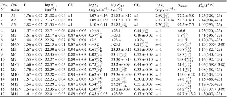
Table 4. Whole XMM-Newton and XMM-Newton+NuSTAR observations: 0.4–10 keV best-fit model (cut-off-PL + soft-excess Comptt emission + pexmon+ scattered component + two partially covering ionized obscurers).
Obs. Obs. Γ log NH,1 Cf1 log ξ1 log NH,2 Cf2 log ξ2 Acomptt χ2red(χ
2/ν)
N. name (cm−2) (erg cm s−1) (cm−2) (erg cm s−1)
1 A1 1.76 ± 0.02 21.38 ± 0.04 ≡1 1.07 ± 0.16 21.82 ± 0.17 ≡1 2.69+0.07 −0.15 72.2 ± 5.8 1.25(528/423) 2 A2 1.79 ± 0.02 21.32 ± 0.03 ≡1 1.05 ± 0.09 22.02 ± 0.07 ≡1 2.72 ± 0.04 58.3 ± 4.0 2.14(904/423) 3 A3 1.82 ± 0.02 21.33 ± 0.04 ≡1 1.10 ± 0.11 21.82+0.13 −0.20 ≡1 2.70 +0.05 −0.19 92.5 ± 7.5 1.40(593/423) 4 M1 1.57 ± 0.07 22.71 ± 0.06 0.84 ± 0.02 <0.66 >23.1 0.44+0.08 −0.16 ≡–1 <6.6 1.23(520/423) 5 M2 1.61 ± 0.07 22.17 ± 0.03 0.87 ± 0.03 0.57+0.03 −0.16 >23.1 0.19 ± 0.02 ≡–1 7.8 +2.3 −2.3 1.41(596/423) 6 M3 1.44 ± 0.08 22.28 ± 0.07 0.78 ± 0.04 <2.5 >23.4 <0.24 ≡–1 <11.5 1.12(473/423) 7 M4N 1.56 ± 0.07 22.13 ± 0.01 0.87 ± 0.01 <–0.2 >23.1 0.21+0.02 −0.06 ≡–1 30.8 +21.6 −2.9 1.15(1555/1348) 8 M5 1.67 ± 0.07 22.30 ± 0.03 0.94 ± 0.02 0.61+0.14 −0.18 23.33 ± 0.11 0.31 ± 0.09 ≡–1 69.8 +25.3 −33.8 1.14(482/423) 9 M6 1.55 ± 0.07 22.35 ± 0.05 0.88 ± 0.03 0.02+0.55 −0.02 23.11 +0.18 −0.42 0.22 ± 0.09 ≡–1 23.3 +21.6 −12.6 1.25(530/423) 10 M7 1.55 ± 0.08 22.27 ± 0.05 0.89 ± 0.03 0.67+0.10 −0.26 23.30 ± 0.13 0.37 ± 0.10 ≡–1 26.01 +19.7 −13.5 1.16(492/423) 11 M8N 1.60 ± 0.05 22.37 ± 0.03 0.87 ± 0.02 0.75+0.08 −0.41 23.2 ± 0.09 0.44 ± 0.05 ≡–1 21.4 +14.3 −12.3 1.03(1392/1348) 12 M9 1.70 ± 0.07 22.29 ± 0.03 0.93 ± 0.02 0.77+0.06 −0.12 23.31 +0.09 −0.12 0.33 ± 0.08 ≡–1 84.1 +68.3 −42.3 1.08(458/423) 13 M10 1.67 ± 0.07 22.28 ± 0.02 0.94 ± 0.02 0.62 ± 0.11 23.36 ± 0.09 0.32 ± 0.08 ≡–1 127.0 ± 48 1.17(503/423) 14 M11 1.57 ± 0.08 22.23 ± 0.04 0.91 ± 0.03 0.57+0.15 −0.24 23.26 +0.11 −0.17 0.30 ± 0.09 ≡–1 74.8 +47.2 −26.8 1.15(488/423) 15 M12 1.54 ± 0.08 22.29 ± 0.05 0.87 ± 0.04 0.54+0.23 −0.54 23.28 +0.12 −0.16 0.35 ± 0.07 ≡–1 30.5 +19.6 −13.4 1.12(475/423) 16 M13N 1.54 ± 0.07 22.35 ± 0.04 0.87 ± 0.01 0.50+0.18 −0.81 23.2 ± 0.09 0.46 ± 0.05 ≡–1 64.2 +26.5 −14.3 1.02(1371/1348) 17 M14 1.61 ± 0.06 22.01 ± 0.05 0.89 ± 0.02 0.85 ± 0.03 >23.39 0.17 ± 0.07 ≡–1 67.7 ± 13.2 1.43(605/423)
which partially obscure the primary power-law continuum, plus the Comptt soft-excess component. Each observation was fit-ted independently letting the parameters of the two ionized ab-sorber(s), the power law (its photon index and normalization), and the normalization of Comptt free to vary.
Best-fit values obtained for all 17 observations are shown in Table 4, and indicate that each observation was well de-scribed by the above best-fit model, where the obscurer is a combination of one mildly ionized (log ξ1 ∼ 0.5–0.8), which
almost totally covers (Cf1 ∼ 0.8–0.9) the source with a col-umn density of log NH1∼ 22.2–22.7 cm−2, plus one cold/neutral
(log ξ2 always less than 0.2, thus fixed at -1) absorber with a
larger column of log NH1 ∼ 23.2−23.4 cm−2, partially
cover-ing (Cf2 ∼ 0.2–0.4) the source. We note that during the first three archival observations, when the source was unobscured, the best-fit parameters of our Cloudy models converged into a two-component warm absorber solution that is consistent with the values reported by the Suzaku data (Krongold et al.2010), and which were considered a good approximation, at low energy resolution, of the multi-temperature warm absorber detected in grating Chandra and XMM-Newton spectra (Andrade-Velazquez et al.2010; Steenbrugge et al.2005; Paper VI). During the cam-paign, our best-fit values are overall in agreement with the av-erage values found by Paper 0 and the independent measure-ments from Di Gesu et al. (2015), except for the much larger value of ξ1 found here with respect to Paper 0 and Paper IV,
who found a log ξ1 = −1.2 ± 0.08. There are multiple possible
reasons for this apparent discrepancy. First, our analysis is per-formed observation-by-observation and accounts for the strong soft X-ray spectral variability, while our earlier analysis in Pa-per 0 reported the time-average values, and PaPa-per IV fixed their ionization parameters to the average values obtained in Paper 0. Second, we used Cloudy and the latest results from Paper V to model the ionized absorbers/emitters, while previous analy-sis in Paper 0 and Paper IV used the xabs model in SPEX. This may have introduced some systematic differences, in particular in modeling the RRC and Fe-UTA (see also Paper V). Finally, as mentioned above (Sect. 4.3.1), weak but statistically significant residuals are left below ∼1 keV, and between 1.8−2.5 keV, which may be attributed to remaining calibration uncertainties of the pn spectra. In Papers 0 and III, the first were fitted by adding a few
emission and absorption lines in the average spectra, while the latter energy band was excluded in their analysis. We tested on the three XMM-Newton+NuSTAR spectra that adding a few ad-hoc emission and/or absorption lines would indeed contribute to decrease the ionization parameter ξ1 down to values (∼0.3)
where it becomes rather unconstrained and degenerate with the other parameters, though maintaining an overall best-fit that is substantially unchanged. We thus attribute to at least one of the above reasons the apparent discrepancy in ξ1, which should not
however have any implication on theanalysis below and which focuses on the variability, i.e. the relative intensity, of the most intense features measured observation by observation. But we stress that the absolute value of this parameter must be consid-ered model- and calibration-dependent, thus poorly constrained, by the present analysis.
To further compare with Papers I, IV, and VII, we also tried to either (i) fix the intensity of the Comptonization component to those values predicted from the measured UV flux, and fol-lowing the UV-soft-X correlation found as given in Paper VII or (ii) to link any of the free parameters (Γ, NH1, Cf1, NH2, Cf2, Acomptt) listed in Table 4 to a same constant value. The fits
al-ways returned significantly worse statistical values (by at least ∆χ2> 10) in at least a few observations, supporting the need for
all those free parameters. The drawback here being that, in some observations, the model is clearly over-fitting the data and yields poorly constrained parameters (e.g. during M3).
We then investigated the time evolution of all those param-eters left free to vary, searching also for trends and correlations among them. In the top of Fig.9, we plot the 7−10 keV flux light curve, since the flux in this energy band should have very lit-tle, if any, sensitivity to the obscuration. Interestingly, the source fluxes between 7−10 keV during the archival observations (first three observations), the average historical values (Paper VI), and during the campaign (last 14 observations) are all comparable within a factor of ∼2. Moreover, except for observation M3, which shows the flattest of all photon index measurements (Γ ∼1.44), all other values of the photon index are within the lower and higher limits (i.e. 1.54−1.79, see Table3) found from the 3 XMM-Newton+ NuSTAR broadband fits, i.e. should really be in-dicative of the intrinsic power-law continuum underlying shape. This readily suggests that most of the flux and spectral variability
0 1 1 0.8 0.9 1 1.1 1.2 Ratio Energy (keV)
Single Obscurer: Full Cov. + Neutral a)
χ2= 13831 0 1 1 0.9 1 1.1 Ratio Energy (keV)
Single Obscurer: Full Cov. + Ionized b)
χ2= 5254 0 1 1 0.9 0.9 5 1 1.0 5 1.1 Ratio Energy (keV)
Single Obscurer: Partial Cov. + Ionized c)
χ2= 4502 0 1 1 0.9 0.9 5 1 1.0 5 1.1 Ratio Energy (keV)
Double Obscurers: 2 Partial Cov. 1 Ionized d)
χ2= 4301 10−6 10−5 10−4 10−3 0.01 keV 2 (Photons cm −2 s −1 keV −1) 0 1 1 0.9 1 1.1 ratio Energy (keV) e)
Fig. 8.Data-to-model ratios (panels a)–d)) of the 3 XMM-Newton+
NuSTARobservations for different models (see text for details) and plot of the unfolded best-fit spectrum of the grouped spectra (panel e)).
5 10 15 10 −11 5×10 −12 Flux (7−10 keV) Observation Number a) 5 10 15 1.4 1.6 1.8 Γ Observation Number b) 5 10 15 21 21.5 22 22.5 23 log N H1 Observation Number c) 5 10 15 0.6 0.7 0.8 0.9 1 Cf1 Observation Number d) 5 10 15 −1 0 1 2 log ξ1 Observation Number e) 5 10 15 21 22 23 24 logNH2 Observation Number f) 5 10 15 0 0.5 1 Cf2 Observation Number g)
Fig. 9.Interesting evolution of the spectral fit parameters versus the
observation number (where, for better clarity, the archival observations are indicated in black, while those from the campaign are indicated in red). From top to bottom: power-law flux between 7−10 keV, Γ, log NH1,
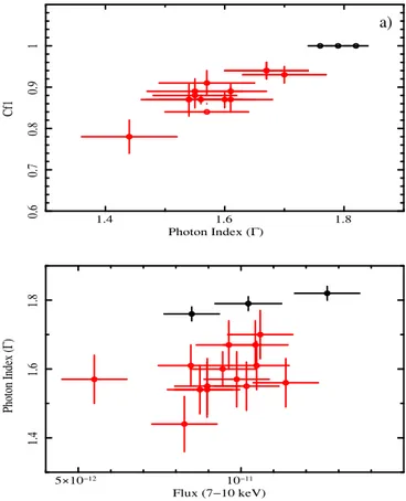
1.4 1.6 1.8 0.6 0.7 0.8 0.9 1 Cf1 Photon Index (Γ) a) 5×10⁻¹² 10−11 1.4 1.6 1.8 Photon Index ( Γ) Flux (7−10 keV)
Fig. 10.(Panel a)) Spectral fit parameters Γ versus Cf1 (panel a)) and
(panel b)) Γ versus power law F7−10 keV (panel b)). Archival
observa-tions are indicated in black, while those from the campaign are indicated in red.
seen at lower energies can be ascribed to the obscurer itself, with only little changes in the intrinsic continuum flux and shape. This is confirmed in panels b to g of Fig. 9, which show the time variability of the most interesting best-fit parameters of the two obscurer(s) as a function of the observation number. This is also confirmed by our independent analysis and model-ing of the fractional variability shown below. Overall, we find only weak (though statistically significant) variations of the ion-ization parameter ξ1, while ξ2 is consistent with being ∼0 (i.e.
neutral gas) since the start of the campaign, from observation M1. We note that, given the complexity of the multi-component spectral model used here, we did not find any single parameter that could be considered as being responsible, alone, for most of the observed spectral variability, but several parameters com-bined to produce the complex spectral variability shown below.
We then looked for trends and correlations among all the best-fit parameters listed in Fig.9. We find only one weak, but significant, correlation between Cf1and Γ, with Cf1' 0.5×Γ+0.1 for a Pearson linear correlation coefficient of 0.94, correspond-ing to a chance probability of <10−5 (see Fig. 10, panel a). The correlation also remains significant after deleting the three archival observations (correlation coefficient of 0.86, chance probability value of 8 × 10⁻⁵). Why would the covering factor,
which is a geometrical factor, depend on the power-law intrinsic shape? This is certainly puzzling and will be addressed later in the discussion (Sect. 5.2). However, another possibility could be that the correlation is driven by an intrinsic degeneracy of the model parameters. A quantitative estimate of this effect would require extensive simulations involving complex models that are beyond the scope of this paper, but this caveat should be kept
Fig. 11.Modelling of the Fvarspectrum using best-fit model and best-fit
parameters of Table4.
in mind. Finally, a general trend (but not a correlation) is also found (see Fig.10, panel b) where the source appears to be sys-tematically intrinsically flatter during the (absorbed) campaign than during the archival (unabsorbed) observations. This point will also be briefly discussed in Sect. 5.2.
4.4. Modeling of the XMM-Newton Fvarspectrum
We used the best fit spectral models during the campaign and described in Sect. 4.3.2 to derive the corresponding Fvarspectra
(Fmodel
var in the following), which we compared with the observed
Fvar spectrum of the campaign shown in Figs. 2 and11in an
attempt to single out the main parameters responsible for the ob-served spectral variability.
We first checked whether our best-fit model can reproduce the Fvar spectrum correctly by letting all the parameters of the
model vary within the corresponding range of best-fit values listed in Table4. The Fmodelvar curve is shown as a red dotted line in
Fig.11. The good agreement between the theoretical and the ob-served Fvardemonstrates, as expected given the Fvarcalculation
definition, that our best-fit spectral model is able to reproduce the correct flux variability at each energy. To obtain the Fmodel
var curve,
the excess variance has been normalized by the total flux (which also includes the contribution from constant components) as a function of energy. This explains the net decrease of variability in the soft band and at ∼6.4 keV, where the constant soft scat-tered component (Sect. 4.2) and the narrow FeK emission line (Sect. 4.1.2) give significant contributions.
Figure 12shows the theoretical Fmodelvar spectra obtained by
varying just one parameter of the best-fit model (or a combina-tion of parameters, normalizacombina-tion, and index, in the case of the power law) and leaving all the others fixed to the best-fit values of observation M7, chosen as a reference for its similarity to the average values. The variable parameter spans the 14 best-fit val-ues listed in Table4. These curves show the energy distribution of the variability power of the main parameters of the model. We note that the only components contributing to the soft band vari-ability are the normalization of the intrinsic soft excess (Acomptt),
and the covering fraction of the mildly ionized obscurer(Cf1). On the other hand, the main parameters contributing to the variabil-ity above ∼1 keV are the column densvariabil-ity of the mildly ionized obscurer, NH1, and the power-law normalization and spectral
in-dex. Interestingly, the Fvar, which was obtained by varying only
Nh1 Cf1 AcompTT Cf2 Nh2 Apow , !
Fig. 12.Spectral decomposition of the different model components
con-tributing to the total Fvarspectrum.
Nh1
Apow
Fig. 13. Spectral decomposition varying only the column density of
component 1 of the obscurer and the power-law normalization between 7−10 keV (see text for details).
the observed Fvar, with a peak at 1−1.5 keV and a sharp drop
in the soft band. We note also that the colder component of the obscurer (NH2and Cf2) brings only weak variability power, and mostly concentrated between 2−4 keV.
We verified whether variations of the NH1 parameter, plus
variations of the normalization of the power law alone (i.e. with-out variation of Γ, the corresponding Fvar being then constant
over the entire energy range), can account for most of the ob-served variability above ∼1 keV. To this aim we combined the theoretical Fvar curves obtained by varying the NH1 parameter
only, and the power law flux in the energy range 7−10 keV (see Fig.13). The 7−10 keV energy range was chosen (rather than the normalization at 1 keV, as given by XSPEC fits) so as to bet-ter constrain the intrinsic variations of the power-law normaliza-tion and avoid spurious contribunormaliza-tion from other parameters (see Fig.12). Figure13shows that most of the observed variability at E > 1 keV can be explained by variations of NH1and
power-law normalization/flux. The residual variability in the soft band might be attributed either to the Comptt component and/or the covering fraction of the mildly ionized obscurer.
A similar model-independent analysis is presented in Pa-per VII for the whole Swift long-term monitoring, which probes typically longer timescales of variability than here, i.e. 10 days up to ∼5 months. For those periods, when the Swift monitoring
10−4 10−3 0.01 keV 2 (Photons cm −2 s −1 keV −1 ) 0.9 1 1.1 ratio 3 4 5 6 7 8 9 10 −5 0 5 10 15 sign(data−model) × ∆ χ 2 Energy (keV) a) b) c)
Fig. 14.The 3–10 keV band unfolded spectrum obtained from the
spec-tra of the 3 XMM-Newton (black) + NuSTAR (in red) simultaneous ob-servations. Spectra (panel a)), the data/model ratio (panel b)), and the residuals in units of ∆χ2(panel c)).
included also the XMM-Newton campaign, the Fvarrecorded by
Swift was consistent in shape with the XMM-Newton one, al-though with significantly lower statistical quality. Swift was not sensitive enough to constrain variations in column density, which was thus fixed at a constant value of 1.2 × 1022cm−2as obtained from the time-averaged data presented in Paper 0, and most of the spectral variability was attributed to variations of the cov-ering fraction of the obscurer only. Moreover, the signature of the NH1variability, the very sharp “drop” below ∼1 keV in the
pn Fvarspectrum, was not apparent in the Swift data either. Given
the lower S/N data and the longer timescales probed by Swift, we consider their results in agreement with the more detailed ones presented here.
4.5. Additional emission and absorption complexities in the Fe K energy band
As mentioned above (Sect. 4.3), after reaching a best-fit broad-band model of the 3 XMM-Newton + NuSTAR observations, we are still left with additional, albeit weak, features in the Fe K en-ergy band, namely one moderately broad emission line feature below 6 keV, and a set of at least two absorption features, around 6.7−6.9 keV and ∼8 keV (see Fig. 14). As shown in Fig.14, these features are seen in both pn (black) and NuSTAR (red), the latter having lower energy resolution but greater effective area than the pn at energies above 7−8 keV. The 6.7−6.9 keV feature was also detected in the MOS, while at higher energies the MOS statistics are not sufficient to either confirm or dis-prove the 8 keV line as well. The features are also seen, and at the same significance, if the background is not subtracted from the source+background spectra. F-tests indicate that both absorption lines are significant (at >99%), with ∆χ2 ∼ 25–30