UNIVERSITÀ DEGLI STUDI DI ROMA
"TOR VERGATA"
FACOLTA' DI INGEGNERIA
DOTTORATO DI RICERCA IN
INGEGNERIA DELL'ENERGIA-AMBIENTE
XXII CICLO DEL CORSO DI DOTTORATO
New Transport Equations for Turbulent flow with variable Transport Properties.
Biomedical Applications of Non-Newtonian Blood Flow in Coronary Stent and
Stenosed Carotid Artery
Andrea Boghi
A.A. 2009/2010
Docente Guida/Tutor: Prof. Fabio Gori
“Big whirls have little whirls, That feed on their velocity, and little whirls have lesser whirls, and so on to viscosity.” Lewis F. Richardson, Weather Prediction by Numerical Process, 1920
Contents
Abstract vii
1 INTRODUCTION 1
1.1 Variable Physical properties 1
1.2 Turbulence Modeling 2
1.3 Second Order Turbulence Closures 3
Nomenclature for Second Order Moments Equations 5
1.4 Second Order Moments equations 7
1.5 Computational Methods 10
References of Chapter 1 12
2 NUMERICAL METHOD 13
2.1 Finite Volume Method (FVM) in a two-dimensional flow 13
2.2 Boundary Conditions 18
2.2.1. Entry conditions: VELOCITY INLET 18
2.2.2. Condition of wall: WALL 20
2.2.3. Output condition: OUTFLOW 21
2.2.4 Pressure condition imposed: CONSTANT PRESSURE 22
2.2.5 Treatment of Edges 22
2.3 Resolution of The System of Equations 22
2.4 Pressure-Velocity Coupling 24
2.6 The SIMPLER Algorithm 27
2.7 The SIMPLEC Algorithm 28
2.8 The PISO Algorithm 28
2.9 Boundary Conditions For Pressure Correction Equation 29
2.9.1 Entry condition: VELOCITY INLET 29
2.9.2 Condition of wall: WALL 29
2.9.3 Output condition: OUTFLOW 29
2.9.4 Pressure condition imposed: CONSTANT PRESSURE 30
2.10 Comparison of Pressure Velocity Coupling Methods 30
2.11 Properties of discretisation schemes 31
2.11.1 Conservativeness 31
2.11.2 Boundedness 31
2.11.3 Transportiveness 32
2.11.4 Assessment of the central differencing scheme 32
2.11.5 UPWIND, HYBRID and POWER-LAW Schemes 33
2.12 Turbulence modelling 33
Nomenclature for k-ε Model 34
2.13 Equations 36
2.14 Grid 37
2.15 Results 38
3 PASSIVE SCALAR EQUATION WITH VARIABLE DIFFUSIVITY IN
TURBULENT FLOW 51
Nomenclature for Passive Scalar equation 51
3.1 Passive scalar equation 52
3.2 Modelling fluctuating diffusivity 55
3.3 Turbulence modelling 57
References of Chapter 3 60
4 ON A NEW PASSIVE SCALAR EQUATION WITH VARIABLE MASS DIFFUSIVITY: FLOW BETWEEN PARALLEL PLATES 61
4.1 Introduction 61
Nomenclature for Mass Transfer Model 66
4.2 Mass diffusion equation 68
4.3 Modelling fluctuating mass diffusivity 69
4.4 Turbulence modelling 71
4.5 Numerical solution and boundary conditions 72
4.6 Results 74
4.7 Discussion on the model 84
4.8 Conclusions 86
5 ON A NEW TURBULENT ENERGY EQUATION WITH VARIABLE
THERMAL CONDUCTIVITY 91
5.1 Introduction 91
Nomenclature for Heat Transfer Model 93
5.2 Energy conservation equations 94
5.3 Modelling the fluctuating Thermal Conductivity 96
5.4 Turbulence modelling 100
5.5 Numerical Model
102
5.6 Results
102
5.7 Discussion On The Model 106
5.8 Conclusions 108
References of Chapter 5 108
6 TWO NEW DIFFERENTIAL EQUATIONS OF TURBULENT DISSIPATION RATE AND APPARENT VISCOSITY FOR NON-NEWTONIAN FLUIDS 112
6.1 Introduction 112
Nomenclature for Non-Newtonian Model 115
6.2 Constitutive equation 116
6.3 Conservation equations of mass, momentum and turbulent kinetic energy 116
6.4 Discussion on the turbulent kinetic energy 118
6.8 Discussion on the conservation equation for the dissipation rate 125
6.9 Order of Magnitude Analysis 127
6.10 Discussion on the equations simplified with the order of magnitude analysis 132
6.11 Conclusions 134
Appendix 135
A. Transport equation for turbulent kinetic energy 135
B. Transport equation for the shear rate 136
C. Transport equation for $2 137
D. Transport equation for the dissipation rate of turbulent kinetic energy 139
E. Order of magnitude analysis of turbulent kinetic energy 142
F. Order of magnitude analysis of the dissipation rate of turbulent kinetic energy 143
References of Chapter 6 153
7 INFLUENCE OF THE NON-NEWTONIAN BEHAVIOUR IN AN IMAGE-BASED COMPUTATIONAL MODEL OF FLOW DYNAMICS IN STENOSED CAROTID ARTERY 157 7.1 Introduction 157 7.2 Model construction 160 7.3 Boundary Conditions 161 7.4 Numerical methods 163 7.5 Results 166
7.5.2 Non-Newtonian Importance Factor 174
7.6 Discussion 178
7.7 Conclusion 181
References of Chapter 7 182
8 THREE-DIMENSIONAL NUMERICAL SIMULATION OF BLOOD FLOW IN TWO CORONARY STENT 185
8.1 Introduction 185
8.2 Geometry 186
8.3 Governing equations 189
8.4 Fluid dynamics parameters 190
8.5 Results 192
8.5.1 Mesh 192
8.5.2 Steady state simulations 193
8.5.3 Unsteady state simulations 196
8.6 Non-Newtonian model 202
8.6.1 Steady State Results 204
8.6.2 Unsteady State Results 205
8.7 Discussion 208
8.8 Conclusions 211
Abstract
Transport properties such as thermal conductivity, mass diffusivity and viscosity of aqueous solutions are important in many industrial processes, scientific applications such as biological processes of living organisms, and in prediction of heat and mass-transfer coefficients under turbulent regimes. Available theoretical models frequently cannot describe real systems as they are met in practice. Better predictive models can be developed based on reliable experimental information on thermodynamic and transport properties. Only few works have dealt with the variability of physical properties in turbulent flow. In the previous models the equations are deduced with the assumption of constant physical properties and later the dependence on the transported variable is introduced. The present paper is aimed to investigate the influence of the variability of physical properties on the transport equations of mean variables and second order moments in turbulent flow. We focus on heat, mass and momentum transfer. As well established in Non-Newtonian fluid mechanics, besides the Reynolds ones, new terms, depending of the variability of physical properties, appear which are involved in energy transfer between large and small scales of turbulence. Concerning mass and heat transfer properties these new terms are achieved, modelled and a FORTRAN Finite Volume code is written to give the order of magnitude of the influence of these terms. Concerning the momentum transfer a new transport equation for turbulent kinetic energy dissipation rate is proposed. In the last two sections we show two examples of Non-Newtonian fluid momentum transfer: blood flow in coronary stent and carotid artery solved by commercial code FLUENT. Despite in the last problem we have turbulent flow, we have treated it in laminar regime because a closure for the turbulent dissipation rate equation proposed in this work is lacking yet.
Keywords: Turbulent Flow, Mass Diffusivity, Thermal Conductivity, Non-Newtonian, Carotid
Introduction
1.1 Variable Physical Properties
Transport properties (thermal conductivity, mass diffusivity and viscosity) of aqueous solutions are important in many industrial processes such as material transport, solid deposition, corrosion in steam generators, and electrical power boilers, and scientific applications such as calculation of design parameters, developments and utilization of geothermal and ocean thermal energy, efficient operation of high-temperature energy-generating systems, geology and mineralogy, hydrothermal synthesis, biological processes of living organisms, and in prediction of heat and mass-transfer coefficients under both laminar and turbulent regimes. Knowledge of pressure, temperature, and composition dependence of transport properties of aqueous electrolyte solutions are essential to understand a variety of problems in a number of technological and engineering applications as: chemical processes, desalination processes, geochemistry, calculation of design parameters, development and utilization of geothermal and ocean thermal energy, geology and mineralogy, prediction of heat and mass-transfer coefficients, environmental applications, and treatment of wastewater.
To understand and to control the processes using electrolyte solutions, requires the knowledge of their thermodynamic and transport properties. Thermal conductivity and viscosity
such systems. Electrostatic interactions govern thermodynamic and transport properties of ionic electrolyte solutions.
Available theoretical models frequently cannot describe real systems as they are met in practice. Better predictive models can be developed based on reliable experimental information on thermodynamic and transport properties. However, measurements of thermal conductivity and viscosity of aqueous salt solutions have so far been limited to rather narrow ranges of temperature, pressure, and concentration with less than satisfactory accuracy [1.1].
1.2 Turbulence Modeling
Much of the efforts in developments of turbulence models focus on ensuring a strict compliance with physical constraints and mathematical formalism, which are “per se” supposed to ensure a higher degree of model generality. Physical constraints are in part identified with the compliance with turbulence asymptotic and limiting states (infinite and vanishing Reynolds numbers, two-dimensional turbulence and others). The ability to reproduce the behavior of individual terms in transport equations for turbulent stresses and scale-supplying variable in various flows is also regarded as a criterion for the validation of physical foundation of the modeling concept.
Some of the mathematical constraints, such as coordinate invariance, are ensured by most second-moment closures. A strict fulfillment of others, such as frame indifference, or various realizable constraints, often imposes a degree of model complexity which aggravates the application of the models to the computation of real flows, although the conditions in which these constraints may come into prominence, are rarely encountered in such flows. The true validation of turbulence models is in their ability to reproduce and predict a wide range of real flows with acceptable accuracy. A compromise is often needed between the strict compliance
with various constraints and computational sturdiness, which will allow the model to be incorporated into an efficient numerical algorithm and applied to the solution of real flows [1.2].
1.3 Second Order Turbulence Closures
Second-order or second-moment turbulence closures which originated with the work of Rotta [1.3], have been extensively used for the numerical simulation of turbulent flows. With turbulence models of this type, the second-moment correlations representing the turbulent transport of momentum, heat or any other scalar are found directly from their own (necessarily approximate) transport equations [1.4]. The approach may be contrasted with the usual phenomenological treatment in which, by analogy with molecular transport, models are devised for the effective turbulent viscosity and effective turbulent Prandtl or Schmidt number.
The transport equations for the second-moments, which serve as the basis for all one-point closures, including eddy-viscosity models, describe in essence the dynamics of large scales, energy-containing motion: the second-moments are of the same order of magnitude as the kinetic energy, providing thus information on the overall characteristic turbulent velocity scale. In order to close the unknown terms in these equations, it is necessary to introduce another scale, in length or time. The most common choice is the scalar dissipation rate of turbulence kinetic energy (or a combination of k and , such as k), because this quantity appears as a sink term in the kinetic energy equation, and its physical interpretation is straightforward. The entire turbulent field is then described by a unique set of the characteristic time and spatial scales. This is one of the major assumptions underlining the one-point statistical turbulence closures.
assumptions are inherent in modeling some of the terms in transport equations, or are invoked when defining some of the model coefficients. This implicitly assumes that all spatial information can be given by a unique length scale for the whole spectrum and that various eddy and the major processes associated with them are linked together by a spectral transfer of energy at a constant rate. Therefore, the dissipation process, acting on small eddies, is assumed to respond with the same characteristic time to any change imposed or occurring on the energy containing eddies located in the large-scale spectrum range. Despite this obvious oversimplification of the realistic spectral dynamics, such an assumption seems to be satisfactory for a wide range of flows of practical interest. That is why the single-scale modeling approach has been so successful ever since the early development.
There are, however, many flows where such a spectral equilibrium is not attained. Typical examples include several non-equilibrium flows, attached and with separation and reattachment, flow impingement and stagnation, longitudinal vortices, secondary motion, swirl, system rotation. These models cannot reproduce satisfactorily the evolution of any flow which departs significantly from equilibrium conditions. Indeed, the rudimentary forms of modeled transport equations with single source and sink terms, tuned in equilibrium flows, do not offer much flexibility. However, the full second-moment closure in differential form may still serve as a sound basis for accounting for the dynamics of each individual stress component. Handling extreme cases when the flow is subjected to strong time or space variation or abrupt changes of external conditions requires further extension of the model to account for various specific phenomena, as well as further refinements of the current models for each term. In order to capture the non-equilibrium dynamics of such flows, it is necessary to introduce different scales by which to describe eddies of different sizes, their evolution and mutual interaction.
Several multiple-scale approaches within the one-point methodology have been proposed in the literature aimed at distinguishing different scales associated with various processes in the dynamics of turbulence. The statistical two-point description of turbulence has been regarded as a convenient mathematical framework for better understanding and modeling of the one-point quantities allowing deriving a transport equation for the Reynolds stress tensor and others second moments, transport equations for the length-scale tensor, providing a better insight in the closure of the classical one-point dissipation equation and develop multiple-scale models. The reason for preferring a second-moment model is that the turbulent interactions which generate the turbulent stresses and heat fluxes can be treated exactly: moreover, for those processes which cannot be so handled, a more rational and systematic set of approximations can be devised than for schemes founded on the notion of effective turbulent transport coefficients.
Nomenclature for Second Order Moments Equations
Symbol Definition SI Unit
Latin
2
i i
k u u Turbulent kinetic energy m2·s-2
2
i i
ku u Instantaneous turbulent kinetic energy m2·s-2
P Mean pressure Pa p Fluctuating pressure Pa 1 1 2 3 j i k ij ij j i k U U U S x x x
1 1 2 3 j i k ij ij j i k u u u S x x x
ij-component of fluctuating rate of shear tensor
s-1
t Time s
i
U i mean velocity component m·s-1
i
u i fluctuating velocity component m·s-1
,
R ij i j
T u u ij-component of Reynolds stress tensor Pa
,
R ij i j
T u u ij-component of instantaneous Reynolds stress tensor
Pa
i
x i coordinate m
Greek
Passive Scalar Diffusivity m2·s-1
2 S Sij ij
Turbulent dissipation rate m2·s-3
2 S Sij ij
Instantaneous turbulent dissipation rate m2·s-3
Molecular kinematic viscosity m2·s-1
Density kg·m-3
Mean passive scalar
Fluctuating passive scalar
Passive Scalar root Mean Square
1 2 j i ij j i U U x x
1 2 j i ij j i u u x x
ij-component of fluctuating rotation rate tensor
s-1
1.4 Second Order Moments equations
In this section we will list the mainly used Second Order Moments equations for an incompressible non-Newtonian fluid in their exact form.
Turbulent Kinetic Energy Conservation equation:
, , , , 1 1 2 k j j k j j k R ij ij R ij k j j j j i ij ij T k k U P t x x P T S T p k T k u u x x S S (1.1)
Turbulent Dissipation Rate Conservation equation:
, , 1 4 8 4 4 1 4 2 2 j j j j kj ik ij kj ik ij kj j k ik ik ij kj ik ij kj j ik j j jk j k j ik ik T U P D t x x S p P S S S S x x S S S S S u S x p T S u x x S S D x x (1.2)Reynolds Stresses Conservation equation: , , 1 2 1 1 i k i k i k i k i k i k i k i u u j i k i k j u u u u u u j j i k u u k j i j ki j j k i u u i k i k u u j j i k j u u T u u u u U P D t x x U U P u u u u p S x x u p u p D x x u u T u u u x 2 k i k j j u u x x (1.3)
Passive Scalar Variance Conservation equation:
, , 2 2 2 2 j j j j j j j j j j j T U P t x x P u x T u x x x (1.4)
Passive Scalar Variance Dissipation Rate Conservation equation: , , 2 2 2 2 2 j j j j j j j k k j k k j j k j k k k j j j j j k j k T U P t x x u U P x x x x x x u u x x x x x x T u x x x x x (1.5)
Passive Scalar Turbulent Flux Conservation equation:
, , 1 1 i i i i i i i i u j i i j u u u j j i u j j i j j i u i i u j j i i j j i u T u u U P D t x x U P u u u p x x x p D x u T u u u x x u x x (1.6)1.5 Computational Methods
Confidence in CFD can be gained only by proving that basic errors of numerical simulations are efficiently reduced, i.e. iteration, discretization and modeling errors. The discretization error, which is the difference between the exact solution of the differential equations and the exact solution of discretized algebraic system of equations, can be reduced by grid refinement and by employing more accurate approximations. The iteration error, which is the difference between the iterative and the exact solution of the algebraic equation systems, can also be reduced to negligible levels. On the modeling side, turbulence models appear to be the largest and the most common source of error in numerical simulation of Reynolds-averaged Navier–Stokes (RANS) equations, because flows in practice are predominantly turbulent.
Therefore to date, the most common turbulence models implemented in CFD codes are of the eddy viscosity type, e.g. standard k , non-linear k and k models. Even though limitations of these models are very well known, they are used due to numerical robustness and the fact that parametric studies do not often require absolute accuracy but rather calculation of relative differences, caused by specific parametric variations [1.5].
Differential second-moment (Reynolds-stress) turbulence closure models (DSM) have long been expected to replace the currently popular eddy viscosity models (EVM) as the industrial standard for Computational Fluid Dynamics (CFD). Yet, despite almost three decades of development and indisputable progress, only a few commercial CFD vendors offer DSM as a modeling option. Even fewer industrial users recognize the natural superiority of the DSM. These models, used and researched mainly within academic community, are still viewed as a development target rather than as a proven and mature technique for solving complex flow phenomena. Moreover, the second-moment closure require careful use and deeper understanding
of the basic features of flows, e.g. many oscillating convergence behaviors during steady state calculations may be related to capturing some transient phenomena and not to the model’s numerical instability, and hence transient calculations are required to obtain numerically and physically accurate results. However, more reliable and refined turbulence models than those of the eddy-viscosity type are clearly required. In the case of the second-moment closure, attempts of using it for complex industrial applications have been reported, but commercial CFD vendors still do not recommend it for ‘everyday’ applications. It seems that so far, a robust numerical algorithm is not available for the second-moment closure.
In the last decade, a number of papers have been reported on the implementation of the second-moment closure in finite volume codes. The starting point of most of the work in this area is the set of governing Reynolds-Averaged Navier–Stokes equations solved for dependent variables in Cartesian co-ordinates and by using collocated variable arrangements. The same approach is also used in many commercial CFD codes, e.g. STAR-CD, FLUENT, CFX, AVL FIRE/SWIFT, etc. The advantages of this approach, like having a single set of computational cells covering a non-orthogonal calculation domain, easier implementation of boundary conditions and general simplicity without diminishing the accuracy of simulations, encourage many CFD developers to follow such practice. Numerical algorithms based on the control volume method often differ in interpolation techniques employed which allow for different types of grids [1.5].
References of Chapter 1
[1.1] I. M. Abdulagatov and N. D. Azizov, Thermal Conductivity and Viscosity of Aqueous K2SO4 Solutions at Temperatures from 298 to 575K and at Pressures up to 30MPa International Journal of Thermophysics, Vol. 26, No. 3, May 2005
[1.2] B. Basara, Employment of the second-moment turbulence closure on arbitrary unstructured grids Int. J. Numer. Meth. Fluids 2004; 44:377–407
[1.3] J. Rotta, Turbulent boundary layers in incompressible flow, in Progress in Aeronautical
Science, Vol. 2. Pergamon, Oxford (1962). 37.
[1.4] B. E. Launder and D. S. A. Samaraweera Application of A Second-Moment Turbulence Closure To Heat And Mass Transport In Thin Shear Flows-I. Two-Dimensional Transport Inf J Hmr, Muss Trunsfir. Vol. 22. Pp 1631-1643
[1.5] A. Cadiou, K. Hanjalić, K. Stawiarski, A two-scale second-moment turbulence closure based on weighted spectrum integration Theoret. Comput. Fluid Dynamics (2004) 18: 1–26
Numerical Method
2.1 Finite Volume Method (FVM) in a two-dimensional flow.
Let list the equations involved in Cartesian coordinates for a Newtonian incompressible fluid with variable diffusivity. The equations have the following form
div u div S t (2.1) The finite volume discretization is treated first in steady case and its generalization to unsteady case is simple. At first the equations are discretized in a FVM approach and the algorithm to solve the pressure-velocity coupling is choosen later. In a FVM approach the integration over a control volume,in a rectangular mesh, givesˆ ˆ dV u ndA ndA S dV t
(2.2)
, , 1 1 , , , , 2 2 1, , , , , , 1, , 1, , , , 1, , 2 ˆ 2 2 ˆ p p I J K i j k I J K i j k I J K I J K I J K I J K I J K i J K j k i J K j k j k j i I J K i dV x y z t t u ndA u x x u x x u x x u x x ndA x x x x x
1, , 2 1, , , , 1, , , , 1, , , , , , 1, , , , 2 2 k I J K I J K I J K I J K I J K I J K I J K I J K I J K j k j k i i I J K x x x x x x x S dV S x y z
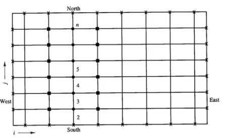
(2.3)The scheme is a second-order Central Difference with the variables calculated on the edges of the control volume with a linear interpolation and a dummy node is considered on the edge, Fig. 2.1. Following Patankar [2.1], the staggered grid is adopted, due to the natural grid for a fluid dynamic problem. For x-velocity, Fig. 2.2, the cell contours in y direction coincide with those of the scalar one, while the contours along x direction are moved to mid-cell along x. For y-velocity, Fig. 2.3, the cell contours along x direction coincide with those of the scalar one, while the contours along y direction are moved to mid-cell along y. For the velocity components a fictitious grid is used, the longitudinal middle column is shifted forward and between the nodes
j ip, p
and
J I, 1
is present the node
J i, p . The transverse node is shifted of a half-1
forward line between the nodes
j i and p, p
J1,I
, i.e.the node is
jp 1,I
.Figure 2.1 Control volume for scalar variables.
, 1, , , , , 1 , 1, 1 1 , , 1, , , , 1 , , 1 1 , , 1 , , , ; ; 2 2 ; ; 2 2 2 p p p p p p p p p p e I J I J e e e j j e i J j j I I w I J I J w w w j j w i J j j I I n I J n n n F a D D y y F u y y x x F a D D y y F u y y x x F a D D
, 1 , , 1 1 1 , , , 1 , , , 1 , , 1 1 , , , , , , , , , , , , , 1, ; 2 ; ; 2 2 p p p p p p p p p p I J i i n I j i i J J s I J I J s s s i i s I j i i J J p e w n s e w n s p I J K e I J x x F v x x y y F a D D x x F v x x y y a a a a a F F F F a a , , 1, , , , 1, , , 1,
1
1
p p p p K aw I J K an I J K as I J K S x i xi yj yj (2.4)Figure 2.2 Control volume for the velocity component (u).
, 1, , 1, , , , 1 , 1 1 , 1, , , , , , 1 , 1 1 , ; ; ; 2 2 ; ; ; 2 2 p p p p p p p p p p p p p p p p i J i J u w I J u w u w u w j j u w j j i i i J i J u e I J u e u e u e j j u e j j i i u s u u F a D D y y F y y x x u u F a D D y y F y y x x a D
1, , , 1, , 1, 1 , 1 , , 1 , 1 1 1, , 1, 1 , 1 1, , , , , 1 , 1 ; ; ; 2 4 2 ; ; 2 4 p p p I j I j u s I J I J I J I J u s u s I I u s I I J J I j u n I J I J I J I J u n u n u n I I u n J J v v F D x x F x x y y v F a D D x x F y y
1 , 1 1 , 1, , , , 1, , , 1 1, 1 , , 1, , , , , , , , , , , , , 1, , 1, , , 1 , ; 2 ; ; p p p p p p p p p p p p p I j I I u u e i J i J u w i J i J u n I j I j u s I j I j u p u e u w u n u s u e u w u n u s u p i J u w i J u e i J u s i J u n v x x b D u u D u u D v v D v v a a a a a F F F F a u a u a u a u a , 1
, 1,
1
p p p i J u I J I J j j u b p p y y (2.5)Figure 2.3 Control volume for the velocity component (v).
1, , , 1, 1 , 1 1, , , , , 1 , 1 1 , , 1 1, 1 , 1, , , , 1 , 1 ; ; ; 2 4 2 ; ; 2 4 p p J i i J v w I J I J I J I J v w v w v w J J v w J J I I J v e I J I J I J I J v e v e v e J J v e I I u u F a D D y y F y y x x u F a D D y y F x x
1, 1 1, 1 , 1 , , , 1 , , , 1 , 1 1 , , , , , , 1 , 1 ; 2 ; ; ; 2 2 ; ; 2 p p p p p p p p p p p p p p i i J J J I j I j v s I J v s v s v s i i v s i i j j I j v n I J v n v n v n i i v n j j u y y y v v F a D D x x F x x y y v F a D D x x F y y
, 1 1 , 1, 1, 1 , , 1, , , 1 , , , , 1 , , , , , , , , , , , , 1, , 1, , , 1 ; 2 ; ; p p p p p p p p p p p p p p p p I j i i v v e i J J i v w i J J i v n I j I j v s I j I j v p v e v w v n v s v e v w v n v s v p I j v e I j v w I j v n I j v v x x b D u u D u u D v v D v v a a a a a F F F F a v a v a v a v a ,s I jv,p bv
pI J, pI J, 1
xip1xip
(2.6)2.2 Boundary Conditions
Implementation of boundary conditions is complicated by the presence of the staggered grid, because many nodes do not coincide with the actual physical boundary of the grid. It is then necessary to borrow the given conditions on the physical boundary-free nodes, i.e. those in the middle between nodes. The presence of staggered grids introduced phantom nodes, where the values of the variables do not need to be calculated.
Boundaries of the passive scalar mesh coincides with the physical contour of the control volume, and nodes surrounding the edges are used for the boundary conditions. It follows that the boundary conditions are introduced changing the discretized equations relative to the nodes adjacent to walls, deleting the link with the boundary nodes and inserting appropriate source terms S and p S . The coefficient of the equation is equal to zero in its boundary and the flow u
that comes from there, exact or linearly approximated, is introduced through Sp and Su. This is
usually done when the flow at a given cell is imposed, but can also be done when is necessary to capture the value in internal nodes of a domain, as, for example, in presence of an obstacle. In that case an arbitrarily large value, like 1030, is imposed to S
p and Su 10 is multiplied by the 30
value of the variable required on that node.
2.2.1. Entry conditions: VELOCITY INLET
The velocity distribution at the entrance of the duct must be specified and the equations must be solved from I , 21 ip . Axial velocity can be imposed by setting the profile
,2 ,
J imposed J
u u (2.7)
The transverse velocity is more complicated because no velocity is present on that node and the source equivalent to the equation I must be solved. In this case it is not necessary to calculate 1
the velocity as the average between a cell and an adjacent one because the value in the middle of the cell is the value to be imposed as boundary conditions. The diffusive and convective terms, relative to the cell, are altered. The convective term is substituted by a fixed flow, and the diffusive term by the gradient calculated on the middle of the cell. Three terms are altered in the equation for v on the node I . 1
, , ,1 1 , 1 , , 1 , , , ,1 1 1 , 1 , , 2, 2, 1 1, 1, 1 , 1, 1 , 1, 1 1, , 1, 1, 0; 2 ; 2 2 2 p p p p p p p p p p p p p p u v j j j in J in J in J in J p v j j j i i in J in J v e J J J J v j i i v n j j v s j S y y u u S y y x x b D u u u u x x D v v D v v
, , ,1 1 1 , , ,1 , , , , , , , , , , ; 0; ; p p p p p u v j j i i v w j v p v e v w v n v s p v v e v w v n v s S x x a a a a a a S F F F F (2.8)Let write the conditions for scalar variables considering two different ones for the passive scalar, i.e. Dirichlet or Neuman type condition.
1 , 1 1 , , , , , , , , , , , , , , 1, , 2, , 1, 1 , 1, 1 , 2 ; ; 0; ; ; p p p p p p j j p in in j j i i u p in w p e w n s p e w n s p J e J n J s J u y y S u y y x x S S a a a a a a S F F F F a a a a S (2.9)2.2.2. Condition of wall: WALL
The most common boundary condition for the two walls, the first for jp and the 1 second for jp Ny . As far as the transverse velocity on the wall is concerned, the boundary 1 conditions are 1,I wall I,1, v v (2.10) 1, , 1, Ny I wall Ny I v v (2.11)
As far as the longitudinal velocity is concerned the equation for J 1 needs to be altered in order to take into account of the value on the wall .
, ,1, , 1 , , ,1, 1 1 , ,1, , 1, 1 2, , 1, 2, 1 , ,2 1,2 1 , ,1, , , , , , , , 0; 2 ; 2 ; 0; p p p p p p p p p p p p p p u u i wall I wall I p u i i i j j u u i u u e i i u w i i u n I I j j u s i u p u e u w u n u s p u u e S S x x y y S b D u u D u u D v v y y a a a a a a S F
Fu w,
Fu n, Fu s,
; (2.12)Let write the conditions for scalar variables.
, , 1 , , ,1, , , , , , , , , , , , ,1 , 1,1 , 1,1 , ,2 , ; 0; 0; ; ; p p u wall I i i p s I p e w n s p e w n s p I e I w I n I u S J x x S a a a a a a S F F F F a a a a S (2.13)2.2.3. Output condition: OUTFLOW
If the output is far from disturbances of geometric type, and the fluid reachs a fully developed flow, the exit condition of type OUTFLOW is implemented. The gradients of all the flow variables are zero in the direction of the main flow except the pressure gradient. The output is placed on the nodes ip Nx , which are immediately following 1 I Nx. The calculations then proceed to ip Nx and 1 I Nx, which are the nodes where the equations require a modification.
, 1 ,
J Nx J Nx
u u (2.14)
The transverse velocity is
, , , 1 , , , 1 , , , 1 1 , , , 1 , , , , 1 1 , , , , , , , , , , , 0; 0; 2 ; 0; ; p p p p p p p p u v p v out J out J v Nx J Nx J v w Nx J Nx J i i u v v n Nx j Nx j v s Nx j Nx j i i v e v p v e v w v n v s p v v e v w v n v s S S b u u D u u x x S D v v D v v x x a a a a a a S F F F F (2.15)
, , , , , , , , , , , , , , , , 1, , , 1 , , 1 , 0; 0; 0; ; ; u p e p e w n s p e w n s p Nx J w Nx J n Nx J s Nx J u S S a a a a a a S F F F F a a a a S (2.16)2.2.4. Pressure condition imposed: CONSTANT PRESSURE
The boundary condition requiring imposition of pressure is used when the values of the pressure boundary are known. Typical problems of this kind are flows on outer surfaces, around objects, free surfaces, buoyancy-driven flows, natural convection, flames propagation, internal flows with multiple outputs. A convenient method of treating this condition is to determine the pressure just inside the edge of the physical domain, that is I , 1 I Nx.
The axial velocity equation is solved from ip to 2 ip Nx, and the other scalar variables from I to 1 I Nx. The main problem is the calculation of the longitudinal velocity because the entry value is determined by the conditions within the domain. This difficulty is resolved by generating a velocity boundary that satisfies the continuity equation.
2.2.5. Treatment of Edges
In dealing with the boundary conditions we must be very careful to what happens in the points of different boundaries, i.e. the edges.
2.3 Resolution of The System of Equations
There are two families of methods: direct ones, which belong to the method of inversion with the Cramer Gauss elimination, and iterative ones. In a direct method the number of operations to solve a system of N equations in N unknowns is of the order of N , because is 3
required the simultaneous storage in memory of all the N variables, the matrix coefficients, for 2 N times..
The iterative methods are based on the repetition of a relatively simple algorithm that leads to convergence after a certain number of calculations. Examples are the algorithms of
Jacobi and Gauss-Seidel. The total number of iterations is N times the number of iterations, not predictable in advance. It is guaranteed in advance the convergence of iterative method, unless meeting certain assumptions. The main advantage of iterative methods is that only non-zero coefficients of the system must be stored in memory, because most of the factors that resolve the system with a direct method are zeros. The methods of Jacobi and Gauss-Seidel are simple to implement, but can lead to slow convergence. In 1949, Thomas proposed a technique to solve tridiagonal systems, called tri-diagonal matrix algorithm (TDMA), which is a direct method for one-dimensional problems, but can be used also for two and three dimensions iteratively. From the computational point of view is very economical and requires a minimum number of variables stored in memory.
The Thomas algorithm consists of two steps: forward-elimination, which consists of eliminating the unknown node's previous system of equations, and back-substitution of a node according to the values of the unknown in the next node.
, , , 1 , , , , , , , , , 1 , , , 1 , , , , , , , 1 , , , 1, , 1, , I J I J I J I J n I J p s I J s I J I J I J p s I J I J e I J w I J u A C a A a a A a C C C a a A C a a S (2.17)
In this system, the boundary conditions must be given. Iterations proceed from J 2 to 1
J Ny , and along x from ip , 2 ip Nx, [2.2].
, ,1 , ,1 0 0 I I A C
Figure 2. 4 Thomas Algorithm.
2.4 Pressure-Velocity Coupling
In this way a system of N equations in N1unknown is written,missing the pressure conservation equation, which is not exhisting. The calculation of pressure, which is a state variable, can be done by the knowledge of other state variables as density and temperature. For example in the case of ideal gases
pRT (2.19)
or for a Van der Waals equation of state
2 1 RT p a b (2.20)
During the iterative calculation the pressure can be obtained once density and temperature are calculated.
For incompressible flow the density is constant and cannot be linked to the pressure and a system of N equations in N unknowns is present. The problems associated with non-linear equations and the coupling between pressure and velocity can be solved by adopting an iterative procedure like that proposed with the SIMPLE algorithm, Patankar and Spalding (1972). In this
algorithm and its later developments, the coefficients of the system are evaluated according to the guessed-variables, which translate into those evaluated during the previous iteration. In this way the coefficients can be calculated and a linear system must be solved. The pressure needs to be estimated in order to make the calculation of velocity, and the pressure correction equation is obtained from the continuity one. The pressure correction equation is used to update pressure and velocity components and the algorithm proceeds until convergence. The estimated variables are marked with an asterisk:
* * * * * * * , , , 1, , 1, , , 1 , , 1 , 1, 1 * * * * * * * , , , 1, , 1, , , 1 , , 1 , , 1 1 * * , , , 1, p p p p p p p p p p p p p p u p i J u w i J u e i J u s i J u n i J u I J I J j j v p I j v e I j v w I j v n I j v s I j v I J I J i i p I J e I J a u a u a u a u a u b p p y y a v a v a v a v a v b p p x x a a a * * * ,w I 1,Ja,n I J, 1a,s I J , 1Su, (2.21)2.5 The SIMPLE Algorithm
The acronym SIMPLE, standing for Semi-Implicit Method for Pressure-Linked Equation, was introduced by Patankar and Spalding in 1972 and is essentially a guess-and-correct procedure.
The variable correction is defined as the difference between the true value of the variable and the variable estimated, therefore
* * * p p p u u u v v v (2.22)
Substituting the correct pressure field equation the correct velocity is obtained. Subtracting Eq. (2.5) to (2.21) and Eq. (2.6) to (2.22) the transport equation linking the variables
, , , 1, , 1, , , 1 , , 1 , 1, 1 , , , 1, , 1, , , 1 , , 1 , , 1 1 p p p p p p p p p p p p p p u p i J u w i J u e i J u s i J u n i J u I J I J j j v p I j v e I j v w I j v n I j v s I j v I J I J i i a u a u a u a u a u b p p y y a v a v a v a v a v b p p x x (2.23)The main approximation of the SIMPLE algorithm is done supposing that the contribution of these terms is negligible as compared to the pressure correction, by writing
, 1, 1 , , , , 1 1 , , p p p p p p I J I J j j i J u p I J I J i i I j v p p p y y u a p p x x v a (2.24)Substituting the expressions into the continuity equation it is obtained a linear equation for the pressure correction.
, , , 1, , 1, , , 1 , , 1 ,
p p I J p w I J p e I J p s I J p n I J I J
a p a p a p a p a p b (2.25)
The coefficients are defined as follows:
* * * * , 1, , 1 , 1 , 1 2 2 1 1 , , , , , , , , 1 2 2 1 1 , , , , , , , 1, , , , , , ; ; ; ; ; p p p p p p p p p p p p p p p p p p p p I J i J i J j j I j I j i i j j j j p w p e u p J i u p J i i i i i p s p n v p j I v p j I p p p w p e p s p n b u u y y v v x x y y y y a a a a x x x x a a a a a a a a a ; (2.25)Note that if the estimated variables are correct, the continuity equation is automatically satisfied, and therefore the source of the pressure correction equation is zero, which means that it is correct. Finally, the simplification made in Eqs. (2.24) does not influence the final solution, because in a convergent solution pressure and velocity must be zero. This simplification is due to
the need to calculate an unknown variable as a function of known variables (guessed ones).
* * * 1 1 new p new old u u new old v v p p p u u u u v v v v (2.26)The α are the coefficients of under-relaxation which are between 0 and 1 and cannot be known in advance. This value must be close to unity for faster convergence, but far away from the unit to have a stable solution [2.1-2.2].
2.6 The SIMPLER Algorithm
The algorithm SIMPLER (SIMPLE Revised), Patankar (1980), is an improved version of SIMPLE. The continuity equation is used to derive a transport equation for the pressure, that will calculate a pressure field satisfying the interim continuity equation. This is done through a different arrangement of the momentum equation. Let
, 1, 1 , , , , , 1 1 , , , ˆ ˆ ˆ ˆ ˆ ˆ p p p p p p p p I J I J j j i J i J u p I J I J i i I j I j v p p p y y u u a p p x x v v a (2.27) * * * * , 1, , 1, , , 1 , , 1 , , * * * * , 1, , 1, , , 1 , , 1 , , ˆ ˆ p p p p p p p p p p u w i J u e i J u s i J u n i J u i J u p v e I j v w I j v n I j v s I j v I j v p a u a u a u a u b u a a v a v a v a v b v a (2.28)Requiring that velocities satisfy the continuity equation
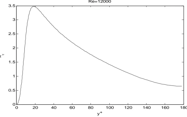
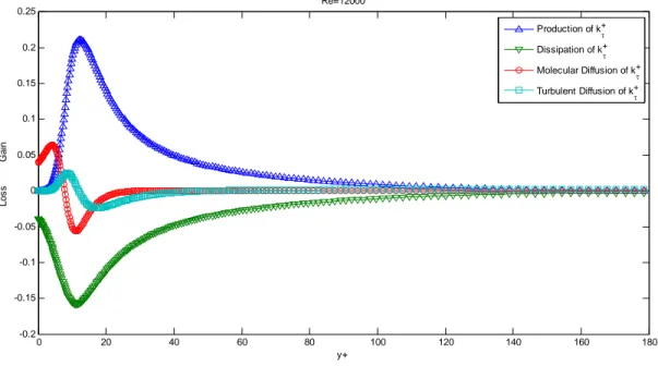
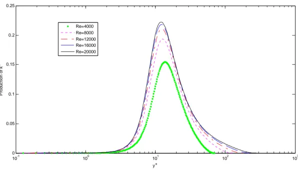
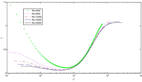
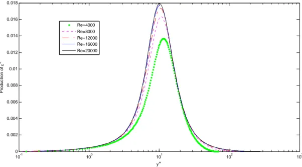
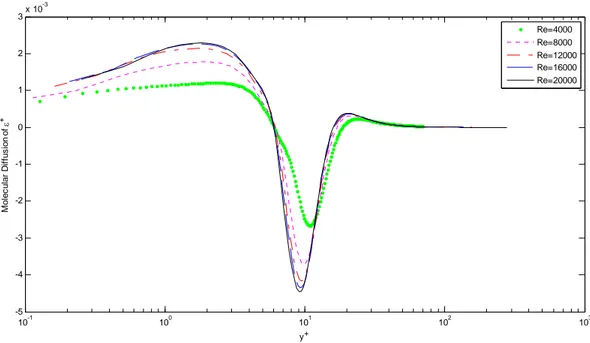
![Figure 2.10 presents the results for Dimensionless turbulent dissipation rate and Figure 2.11 those for Dimensionless turbulent kinetic energy, both comparable with [2.6-2.8]](https://thumb-eu.123doks.com/thumbv2/123dokorg/7600316.114270/49.918.167.777.524.929/figure-presents-dimensionless-turbulent-dissipation-dimensionless-turbulent-comparable.webp)