An Approximate KAM-Renormalization-Group Scheme for
Hamiltonian Systems
C. Chandre1, H. R. Jauslin1, and G. Benfatto2
1Laboratoire de Physique, CNRS, Universit´e de Bourgogne, BP 400, F-21011 Dijon, France 2Dipartimento di Matematica, Universit`a di Roma “Tor Vergata”, Via della Ricerca Scientifica,
I-00133 Roma, Italy (July 25, 2011)
Abstract
We construct an approximate renormalization scheme for Hamiltonian systems with two degrees of freedom. This scheme is a combination of Kolmogorov-Arnold-Moser (KAM) theory and renormalization-group tech-niques. It makes the connection between the approximate renormalization procedure derived by Escande and Doveil, and a systematic expansion of the transformation. In particular, we show that the two main approximations, consisting in keeping only the quadratic terms in the actions and the two main resonances, keep the essential information on the threshold of the breakup of invariant tori.
PACS numbers: 05.45.+b, 64.60.Ak
I. INTRODUCTION
In 1981, Escande and Doveil [1] set up an approximate renormalization scheme for Hamil-tonian systems with two degrees of freedom, in order to study the breakup of invariant tori, and especially to compute the threshold of stochasticity. Their scheme was motivated by Chirikov’s resonance overlap criterion [2], and by Greene’s results [3] about the link between the existence of a torus with the stability of neighboring periodic orbits. They established the relevance of a sequence of these periodic orbits for the breakup of invariant tori, by set-ting an approximate transformation which focuses successively on smaller scales, i.e. acset-ting like a microscope in phase space.
Due to the complexity of the phase space of a non-integrable Hamiltonian, their method re-quires strong approximations to obtain explicit expressions. Basically, two approximations were involved:
(1) a quadratic approximation in the actions: their transformation produces terms that are higher than quadratic in the actions; in order to remain in the same class of Hamiltonians, they neglect these higher order terms,
(2) a two-resonance approximation: they only keep the two main resonances at each itera-tion of the transformaitera-tion.
The idea was to keep only the most relevant features of the mechanism of the breakup of a given torus.
In this article, we construct an approximate scheme using the same two approximations. We establish the connection between Escande’s scheme [1,4] and the KAM-RG transformation derived in Refs. [5–7]. The aim is to show that an exact renormalization transformation can be approximated by a simple transformation: It can be useful to derive approximate explicit expressions of universal parameters, and to see what are the most relevant terms responsible for the breakup of invariant tori. The results we obtain support the general idea that the irrelevant terms of the renormalization transformation can be eliminated with little loss of accuracy in the parameters associated to the breakup of invariant tori.
The transformation R we define has two main parts: a KAM transformation which is a canonical change of coordinates that reduces the size of the perturbation from ε to ε2, and a renormalization transformation which is a combination of a shift of the resonances and a rescaling of momentum and energy.
It acts on the following class of Hamiltonians with two degrees of freedom, quadratic in the action variables A = (A1, A2), and described by three even scalar functions of the angles
φ = (φ1, φ2):
H(A, φ) = 1
2(1 + m(φ)) (Ω· A) 2 + [ω
0+ g(φ)Ω]· A + f(φ), (1.1)
where m, g, and f are of zero average. The vector ω0 is the frequency vector of the consid-ered torus and Ω = (1, α) is some other constant vector not parallel to ω0. The perturbation (m, g, f ) is of order O(ε).
The renormalization-group approach is based on the following general picture: The idea is to construct the transformation R as a generalized canonical change of coordinates acting on some space of Hamiltonians such that the iteration ofR converges to a fixed point. If the perturbation is smaller than critical,R should converge to a Hamiltonian of type (1.1) with (m, g, f ) = 0, which is integrable, and the equations of motion show that the torus with fre-quency vector ω0 is located at A = 0. All Hamiltonians attracted by this trivial fixed point have an invariant torus of that frequency (this can be considered as an alternative version of the KAM theorem [8]). If the perturbation is larger than critical, the system does not have a KAM torus of the considered frequency and the iteration of R diverges. The domain of convergence to the trivial fixed point and the domain of divergence are separated by a critical
surface invariant under the action ofR. The main hypothesis of the renormalization-group
approach is that there should be another nontrivial fixed point (or more generally, a fixed set) on this critical surface, that is attractive for Hamiltonians on that surface. From its existence, one can expect to deduce universal properties in the mechanism of the breakup of invariant tori.
results in the perturbative regime [8], by numerical works [6,7,9,10], and by analogies with the related problem for area-preserving maps [11,12]. In particular, the relation between the properties of the nontrivial renormalization fixed point and the geometric properties of the invariant torus at the instability threshold are not well established. The coincidence of the critical coupling of one-parameter families at which a torus breaks up, with the boundary of attraction of the trivial fixed point is supported by numerical studies [6,7,9].
In Sec. II, we describe the KAM part of the transformation, and we make explicit the two approximations involved in this scheme: the quadratic approximation and the two-resonance approximation. In Sec. III, we present the renormalization transformation which is a combination of the KAM part, a shift of the resonances, and rescalings of actions and energy. In Sec. IV, we give our numerical results, and in particular, we show that the approximate scheme contains the essential features of the exact one.
II. KAM TRANSFORMATION
We perform a canonical transformation UF : (φ, A) 7→ (φ′, A′) defined by a generating
function F (A′, φ) [13,14] characterized by a scalar function X of the action and angle
variables, of the form
F (A′, φ) = A′· φ + X(A′, φ), (2.1) leading to A = ∂F ∂φ = A ′+ ∂X ∂φ, (2.2) φ′ = ∂F ∂A′ = φ + ∂X ∂A′. (2.3)
The function X is constructed such that inH ◦ UF the perturbation terms of first order in ε
are equal to zero. Inserting Eq. (2.2) into Hamiltonian (1.1), one obtains the expression of the Hamiltonian in the mixed representation of new action variables and old angle variables:
˜ H(A′, φ) = (Ω· A′)2/2 + ω0· A′+ ω(A′)· ∂X ∂φ + h(A ′, φ) +O(ε2), (2.4) where ω(A′) = ω0+ (Ω· A′)Ω, (2.5) h(A′, φ) = 1 2m(φ)(Ω· A ′)2+ g(φ)Ω· A′+ f (φ). (2.6)
The equation that determines X is thus:
ω(A′)· ∂X
∂φ + h(A
′, φ) = 0. (2.7)
We recall that the functions m, g, and f are of order O(ε); as a consequence, X is also of order O(ε). Equation (2.7) has the solution
X(A′, φ) = ∑
ν∈Z2
Xν(A′) sin(ν· φ), (2.8)
where, if we write h(A, φ) =∑νhν(A) cos(ν· φ),
Xν(A′) =−
hν(A′)
ω(A′)· ν. (2.9)
The denominator of Xν depends on the actions: thus, by power expansion, it generates
terms that are higher than quadratic in the actions. In order to remain in the same space of Hamiltonians (1.1), we expand the Hamiltonian to the second order in the actions and ne-glect the order O(A3). The justification for such an approximation is that we are interested in the torus with frequency vector ω0 which is located at A = 0 for the trivial fixed point. We consider Hamiltonians (1.1) with only two Fourier modes which are the two main reso-nances defined as follows: For a frequency vector ω0, the resonances are given by the vectors
νn = (pn, qn) which are the sequence of the best rational approximations. They are
char-acterized precisely by the following property: |ω0 · νn| < |ω0· ν|, for any ν ≡ (p, q) ̸= νn
such that |q| < qn+1. For the frequency vector ω0 = (1/γ,−1) with γ = (1 +
√
5)/2, we define the two main resonances as ν1 = (1, 0) and ν2 = (1, 1). Well known properties of continued fractions (see, for example, [15]) imply that the vectors νn satisfy the recursion
relation νn+1 = N νn, where N = 1 1 1 0 .
The scalar functions m, g and f will have expressions of the form
f (φ) = fν1cos(ν1· φ) + fν2cos(ν2· φ). (2.10)
The KAM part of the transformation R will generate a large set of Fourier modes from these two main resonances. The purpose of the renormalization is to relate these two main resonances representing the main scale, to the next pair of resonances (called the daughter
resonances) representing the next smaller scale. For the frequency vector ω0 = (1/γ,−1),
the daughter resonances are ν3 = (2, 1) and ν4 = (3, 2). As the canonical transformation (2.2)-(2.3) is linear in cos(ν · φ) and sin(ν · φ), νn = νn−1 + νn−2 and the three scalar
functions (m, g, f ) are of orderO(ε), the lowest order to which the resonances ν3 and ν4 are produced, is respectively O(ε2) and O(ε3). Thus we neglect the order O(ε4) of the KAM transformation.
The next step is to express the Hamiltonian in the new angle variables using Eq. (2.3). We notice that this equation has to be inverted. As we need the Hamiltonian expressed in the new coordinates to order O(ε3), we have to invert Eq. (2.3) up to order O(ε), since the functions to be expressed in the new angles are already of orderO(ε2). Moreover, these new angle variables depend on the actions, which we develop to order O(A2). The development can thus be summarized by expressing cos[ν.φ(φ′)] as a function of cos(ν.φ′) and sin(ν.φ′), neglecting the orders O(ε2, A3).
The final step is a translation in the A′ variables such that the linear term is again of the form ω0· A′.
The Hamiltonian expressed in the new variables becomes:
H′(A′, φ′) = 1
2(Λ + m
′(φ′)) (Ω· A′)2+ (ω
0+ g′(φ′)Ω)· A′+ f′(φ′), (2.11) where m′, g′ and f′ are given as functions of m, g and f . The constant Λ results of the fact that the mean value of m′ is required to be equal to zero. We notice that the KAM
transformation does not change Ω = (1, α).
The two-resonance approximation consists in retaining only the two daughter resonances and neglect all the other Fourier modes. Therefore the approximate KAM transformation
˜
UF is a map acting on a low-dimensional space of Fourier coefficients:
˜
UF (1; mν1, gν1, fν1; mν2, gν2, fν2) = (
Λ; m′ν3, g′ν3, fν′3; m′ν4, gν′4, fν′4). (2.12) The explicit expression of this map is given in the Appendix.
III. RENORMALIZATION TRANSFORMATION
We construct the approximate transformation by combining two parts: a KAM transfor-mation (m, g, f, α)7→ (m′, g′, f′, α) as defined above, and a renormalization (RG) consisting
of a shift of the resonances and a rescaling of the actions and of time (m′, g′, f′, α) 7→
(m′′, g′′, f′′, α′). The renormalization scheme described in this section is for a torus of fre-quency vector ω0 = (1/γ,−1) where γ = (1 +
√
5)/2. It is straightforward to adapt it to quadratic irrationals.
The approximate KAM-RG transformation is composed of four steps:
1) a KAM transformation described in the previous section, which is a change of coordinates that eliminates terms of orderO(ε), where ε is the size of the perturbation; this transforma-tion produces terms of orderO(ε2), terms that are higher than quadratic in the actions, and a large set of Fourier modes. We neglect terms of orderO(A3, ε4), and also, all the Fourier modes except the two daughter resonances ν3 and ν4. We notice that this transformation does not change Ω.
2) a shift of the resonances: a canonical change of coordinates that maps the pair of daughter resonances (ν3, ν4) into the two main resonances (ν1, ν2).
3) a rescaling of energy (or equivalently of time).
4) a rescaling of the action variables (which is a generalized canonical transformation). The aim of this transformation is to treat one scale at the time. The steps 2), 3) and 4) are
implemented as follows: The two main resonances (1, 0) and (1, 1) are replaced by the next pair of daughter resonances (2, 1) and (3, 2), i.e. we require that cos[(2, 1)·φ′] = cos[(1, 0)·φ′′] and cos[(3, 2)· φ′] = cos[(1, 1) · φ′′]. This change is done via a canonical transformation (A′, φ′)7→ (N−2A′, N2φ′) with N2 = 2 1 1 1 .
This linear transformation multiplies ω0 by γ−2 (since ω0 is an eigenvector of N ); therefore we rescale the energy by a factor γ2in order to keep the frequency fixed at ω0. A consequence of the shift of the resonances is that Ω is changed into Ω′ = (1, α′), where α′ = (α+1)/(α+2). Then we perform a rescaling of the action variables: we change the Hamiltonian H′ into
ˆ H′(A′, φ′) = λH′ ( A′ λ , φ ′ )
with λ such that Hamiltonian (2.11) becomes of the form (1.1). Since the rescal-ing of energy and the shift N2 transform the quadratic term of the Hamiltonian into
γ2(2 + α)2[Λ + m′(φ′)](Ω′ · A′)2/2, this condition leads to λ = γ2(2 + α)2Λ. This con-dition has the following geometric interpretation in terms of self-similarity of the resonances close to the invariant torus: the rescaling magnifies the size of the daughter resonances, and places them approximately at the location of the original main resonances [7].
In summary, the renormalization rescales m, g, f and Ω = (1, α) into
m′′(φ) = m ′(N−2φ) Λ , (3.1) g′′(φ) = γ2(2 + α)g′(N−2φ), (3.2) f′′(φ) = γ4(2 + α)2Λf′(N−2φ), (3.3) α′ = 1 + α 2 + α. (3.4)
The iteration of the transformation (3.4) converges to α∗ = γ−1. It means that Ω converges under successive iterations to Ω∗ = (1, 1/γ), which is orthogonal to ω0 and is the unstable eigenvector of N2 with the largest eigenvalue γ2.
IV. DETERMINATION OF THE CRITICAL COUPLING; AN APPROXIMATE NONTRIVIAL FIXED POINT
We start with the same initial Hamiltonian as in Refs. [4,6,7]
H(A, φ) = 1 2(Ω· A) 2+ ω 0 · A + εf(φ) , (4.1) where Ω = (1, 0), ω0 = (1/γ,−1), γ = (1 + √ 5)/2, and a perturbation f (φ) = cos(ν1· φ) + cos(ν2· φ), (4.2) where ν1 = (1, 0) and ν2 = (1, 1).
We take successively larger coupling ε, and determine whether the approximate KAM-RG iteration converges to a Hamiltonian with (m, g, f ) = 0, or whether it diverges (m, g, f )→
∞. By a bisection procedure, we determine the critical coupling εc = 0.02885. As a
comparison, Escande’s scheme [4] gives εc = 0.02908. The KAM-RG transformation [6,7,9]
yields εc= 0.02759 (Greene’s criterion gives also εc = 0.02759). The two-resonance scheme
gives the result within 5%. Thus, the approximate scheme gives a fairly good description of the critical surface of the breakup of the torus.
The renormalization operator has two fixed points: a trivial fixed point which corresponds to the Hamiltonian H(A, φ) = (Ω∗· A)2/2 + ω
0· A, and a nontrivial fixed point which lies on the boundary of the basin of attraction of the trivial fixed point. The critical surface which is the stable manifold of the nontrivial fixed point is of codimension 1. The relevant critical exponent is δ = 2.7135. This value is close to the one obtained by Escande et al. [16]
δ = 2.7480, or by KAM-RG schemes [9,10] δ = 2.6502, and by MacKay for area-preserving
maps [11] δ = 2.6502.
The fact that δ is close to γ2can be understood by the following heuristic arguments: To the first main resonance ν1 corresponds a Fourier component M exp[i(1, 0)·φ], and to the second one P exp[i(1, 1)· φ]. The first daughter resonance ν3 is represented by M′exp[i(2, 1)· φ]. The transformation is a polynomial change of coordinates that generates a set of Fourier
modes from the two main resonances. The way to generate the first daughter resonance at the lowest order is to combine one resonance ν1 and one resonance ν2. For the second daughter resonance, the change of coordinates must combine one resonance ν1 and two resonances ν2. We rescale the phase space in such a way that the daughter resonances become of the same size as the main resonances. These arguments give the following renormalization relations:
M′ = k1M P, (4.3)
P′ = k2M P2, (4.4)
where k1 and k2 are two constants that depend on how the transformation is performed. An analysis of this scheme shows that it has two fixed points: a trivial one M = 0, P = 0 and a nontrivial one M∗ = k1k−12 , P∗ = k1−1. The nontrivial fixed point has a stable manifold of codimension 1 characterized by a relevant critical exponent; the only eigenvalue greater than one of the linearized map at the nontrivial fixed point is δ = γ2. This relevant critical exponent does not depend on k1 and k2. This is in agreement with the general ideas of the renormalization group. Also, it shows that the relevant critical exponent of the approximate and exact KAM-RG transformation should be expected to be close to γ2.
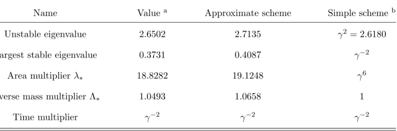
For the scaling factor at the nontrivial fixed point, we obtain numerically λ∗ = 19.1248. This value can be compared with λ∗ = 18.8282 obtained in Refs. [17,18,11,9,10]. Table 1 lists some of the universal parameters associated with the breakup of golden tori.
The approximate renormalization transformation has another fixed set which is a cycle of period three as it had also been encountered in area-preserving maps [12,19] and in the KAM-RG transformation [7]. This cycle is simply related to the nontrivial fixed point by symmetries. In particular, it belongs to the same universality class as the fixed point.
ACKNOWLEDGMENTS
We thank A. Celletti for providing the program to determine the critical coupling by Greene’s criterion. We acknowledge useful discussions with G. Gallavotti, R. S. MacKay, and
H. Koch. Support from EC contract No. ERBCHRXCT94-0460 for the project “Stability and universality in classical mechanics” and from the Conseil R´egional de Bourgogne is acknowledged.
APPENDIX: TWO-RESONANCE SCHEME FORMULAE
We denote cν = cos(ν· φ), c′ν = cos(ν· φ′), and s′ν = sin(ν· φ′). The expression of the
Hamiltonian in the mixed representation of new actions and old angles is
˜ H(A′, φ) = 1 2(Ω· A ′)2+ ω 0· A′ +∑ ν1,ν2 Pν1ν2(A ′)c ν1cν2 + ∑ ν1,ν2,ν3 Qν1ν2ν3(A ′)c ν1cν2cν3, (4.5) where
Pν1ν2(A) = Ω· ν1Xν1(A) [Ω· ν2Xν2(A)/2 + gν2 + mν2Ω· A] , (4.6)
Qν1ν2ν3(A) = Ω· ν1Ω· ν2Xν1(A)Xν2(A)mν3/2. (4.7)
We recall that X is of order O(ε), and is given by Eq. (2.9); as a consequence, P is of order
O(ε2), and Q is of order O(ε3).
Next, the expression of this Hamiltonian in the new angles requires the inversion of Eq. (2.3) to the order O(ε). The expression of cν as a function of s′ν and c′ν is
cν1 = c ′ ν1 + ∑ ν2 Rν1ν2(A ′)s′ ν1s ′ ν2 +O(ε 2 ), (4.8) where Rν1ν2(A) = ν1· ∂Xν2 ∂A .
The Hamiltonian (1.1) expressed in the new variables becomes
H′(A′, φ′) = 1 2(Ω· A ′)2+ ω 0· A′ +∑ ν1,ν2 Pν1ν2c ′ ν1c ′ ν2 + ∑ ν1,ν2,ν3 Qν1ν2ν3c ′ ν1c ′ ν2c ′ ν3 + ∑ ν1,ν2,ν3 (Pν1ν2 + Pν2ν1)Rν2ν3c ′ ν1s ′ ν2s ′ ν3 +O(ε 4). (4.9)
The next approximation is the Taylor expansion of H′(A′, φ′) to the second order in the actions e.g. Pν1ν2(A) = P (0) ν1ν2 + P (1) ν1ν2Ω· A + P (2) ν1ν2(Ω· A) 2+O(A3). (4.10)
In the next step, we neglect all the resonances different from the daughter resonances (2, 1) and (3, 2) using the following relations
c′ν1c′ν2 = 1 2 ( c′ν1+ν2 + c′ν1−ν2), (4.11) c′ν1s′ν2s′ν3 = 1 4 ( c′ν1+ν2−ν3+ c′ν1−ν2+ν3 − c′ν1+ν2+ν3 − cν′1−ν2−ν3), (4.12) c′ν1c′ν2c′ν3 = 1 4 ( c′ν1+ν2−ν3 + c′ν1−ν2+ν3 + c′ν1+ν2+ν3 + cν′1−ν2−ν3). (4.13)
In the following formulas, the subscripts 1, 2, 3 and 4 denote respectively the resonances (1, 0), (1, 1), (2, 1), and (3, 2). The Hamiltonian (4.9) becomes
H′(A′, φ′) = 1 2(Ω· A ′)2 + ω0· A′ + 1 2(P11+ P22) +1 2(P12+ P21)c ′ ν3 + 1 4(Q221+ Q212+ Q122− S122)c ′ ν4, (4.14)
where S122 = 2P22R21+ (P21+ P12)(R12+ R22). Equation (4.14) gives the expression of the Fourier coefficients of the daughter resonances
Λ = 1 + P11(2)+ P22(2), (4.15) m′ν 3 = P (2) 12 + P (2) 21 , (4.16) m′ν4 = 1 2 ( Q(2)221+ Q(2)212+ Q(2)122− S122(2) ) , (4.17) g′ν3 = 1 2 ( P12(1)+ P21(1) ) , (4.18) g′ν4 = 1 4 ( Q(1)221+ Q(1)212+ Q(1)122− S122(1) ) , (4.19) fν′3 = 1 2 ( P12(0)+ P21(0) ) , (4.20) fν′4 = 1 4 ( Q(0)221+ Q(0)212+ Q(0)122− S122(0) ) . (4.21)
TABLES
TABLE I. Universal parameters associated with the breakup of the golden mean torus.
Name Value a Approximate scheme Simple scheme b
Unstable eigenvalue 2.6502 2.7135 γ2 = 2.6180
Largest stable eigenvalue 0.3731 0.4087 γ−2
Area multiplier λ∗ 18.8282 19.1248 γ6
Inverse mass multiplier Λ∗ 1.0493 1.0658 1
Time multiplier γ−2 γ−2 γ−2
agiven in Refs. [12,4] bderived in Refs. [4,16]
REFERENCES
[1] D. F. Escande and F. Doveil, J. Stat. Phys. 26, 257 (1981).
[2] B. V. Chirikov, Phys. Rep. 52, 263 (1979).
[3] J. M. Greene, J. Math. Phys. 20, 1183 (1979).
[4] D. F. Escande, Phys. Rep. 121, 165 (1985).
[5] G. Gallavotti and G. Benfatto (unpublished, 1987).
[6] M. Govin, C. Chandre, and H. R. Jauslin, Phys. Rev. Lett 79, 3881 (1997).
[7] C. Chandre, M. Govin, and H. R. Jauslin, Phys. Rev. E 57, 1536 (1998).
[8] H. Koch, archived in mp [email protected], #96-383. To appear in Erg. Theo. Dyn. Syst. (1998).
[9] C. Chandre, M. Govin, H. R. Jauslin, and H. Koch, Phys. Rev. E 57, XXX (1998).
[10] J. J. Abad, H. Koch, and P. Wittwer, archived in mp [email protected], #98-261.
[11] R. S. MacKay, Physica D 7, 283 (1983).
[12] R. S. MacKay, Renormalisation in Area-preserving Maps (World Scientific, 1993).
[13] H. Goldstein, Classical Mechanics (Addison-Wesley, Reading, Mass., 1980).
[14] G. Gallavotti, The Elements of Mechanics (Springer-Verlag, New York, 1983).
[15] H. Davenport, The Higher Arithmetic (Dover, New York, 1983).
[16] D. F. Escande, M. S. Mohamed-Benkadda, and F. Doveil, Phys. Lett. A 101, 309 (1984).
[17] L. P. Kadanoff, Phys. Rev. Lett. 47, 1641 (1981).
[18] S. J. Shenker and L. P. Kadanoff, J. Stat. Phys. 27, 631 (1982).