Deep Learning Based Robotic Tool Detection and Articulation Estimation with Spatio-Temporal Layers

(1)

Deep learning based robotic tool detection and

articulation estimation with spatio-temporal layers

Emanuele Colleoni

1∗

, Sara Moccia

2∗

, Xiaofei Du

3

, Elena De Momi

1

, Senior Member, IEEE,

Danail Stoyanov

3

, Member, IEEE

Abstract—Surgical-tool joint detection from laparoscopic im-ages is an important but challenging task in computer-assisted minimally invasive surgery. Illumination levels, variations in background and the different number of tools in the field of view, all pose difficulties to algorithm and model training. Yet, such challenges could be potentially tackled by exploiting the temporal information in laparoscopic videos to avoid per frame handling of the problem. In this paper, we propose a novel encoder-decoder architecture for surgical instrument joint detection and localization that uses 3D convolutional layers to exploit spatio-temporal features from laparoscopic videos. When tested on benchmark and custom-built datasets, a median Dice similarity coefficient of 85.1% with an interquartile range of 4.6% highlights performance better than the state of the art based on single-frame processing. Alongside novelty of the network architecture, the idea for inclusion of temporal information appears to be particularly useful when processing images with unseen backgrounds during the training phase, which indicates that spatio-temporal features for joint detection help to generalize the solution.

Index Terms—Surgical-tool detection, medical robotics, com-puter assisted interventions, minimally invasive surgery, surgical vision.

I. INTRODUCTION

M

INIMALLY invasive surgery (MIS) has become the preferred technique to many procedures that avoids the major drawbacks of open surgery, such as prolonged patient hospitalization and recovery time [1]. This, however, comes at the cost of a reduced field of view of the surgical site, which potentially affects surgeons’ visual understanding, and similarly restricted freedom of movement for the surgical instruments. [2]. To improve the surgeons’ ability to perform tasks and precisely target and manipulate the anatomy, it is crucial to monitor the relationship between the surgical site and the instruments within it to facilitate computer assisted interventions (CAI).

Manuscript received: February, 24, 2019; Revised: April, 27, 2019; Ac-cepted: April, 27, 2019.

This paper was recommended for publication by Editor Pietro Valdastri upon evaluation of the Associate Editor and Reviewers’ comments.

*These authors equally contributed to the paper

1_{E. Colleoni and E. De Momi are with the Department of} Electron-ics, Information and Bioengineering, Politecnico di Milano, Milan (Italy) emanuele1.colleoni@mail.polimi.it

2_{S. Moccia is with the Department of Information Engineering, Universit`a} Politecnica delle Marche, Ancona (Italy) and the Department of Advanced Robotics, Istituto Italiano di Tencologia, Genoa (Italy)

3_{X. Du and D. Stoyanov are with the Wellcome/EPSRC Centre for} Interventional and Surgical Sciences (WEISS) and the UCL Robotics Institute, University College London (UCL), London (UK)

Digital Object Identifier (DOI): see top of this page.

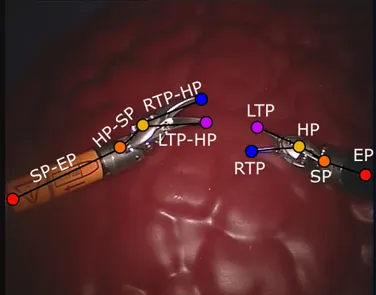
Fig. 1: Each surgical tool is described by five joints (coloured dots) and four connections (black lines). LTP: Left Tip Point, RTP: Right Tip Point, HP: Head point, SP: Shaft point and EP: End Point.

CAI promises to provide surgical support through advanced functionality, robotic automation, safety zone preservation and image guided navigation. However, many challenges in algorithm robustness are hampering the translation of CAI methods relying on computer vision to the clinical practice. These include classification and segmentation of organs in the camera field of view (FoV) [3], definition of virtual-fixture algorithms to impose a safe distance between surgical tools and sensitive tissues [4], and surgical instrument detection, segmentation and articulated pose estimation [5], [6].

Surgical-tool joint detection in particular has been investi-gated in recent literature for different surgical fields, such as retinal microsurgery [7] and abdominal MIS [8]. Information provided by algorithms can be used to provide analytical reports, as well as, as a component within CAI frameworks. Early approaches relied on markers on the surgical tools [9] or active fiducials like laser pointers [10]. While practical, such approaches require hardware modifications and hence are more complex to translate clinically but also they inherently still suffer from vanishing markers or from occlusions. More recent approaches relying on data driven machine learning such as multiclass boosting classifiers [11], Random Forests [12] or probabilistic trackers [13] have been proposed. With the

(2)

This article has been accepted for publication in a future issue of this journal, but has not been fully edited. Content may change prior to final publication. Citation information: DOI 10.1109/LRA.2019.2917163, IEEE Robotics and Automation Letters

2 IEEE ROBOTICS AND AUTOMATION LETTERS. PREPRINT VERSION. ACCEPTED MAY, 2019

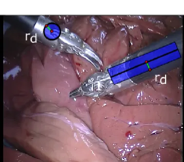
Fig. 2: Ground-truth example for shaft point (circle) and shaft-end point connection (rectangle). We used the same pixel number (rd) for both circle radius and rectangle thickness,

highlighted in green.

increasing availability of large datasets and explosion in deep learning advances, the most recent work utilizes Fully Con-volutional Neural Networks (FCNNs) [5], [14]. Despite the promising results using FCNNs, a limitation is that temporal information has never been taken into account, despite the potential for temporal continuity as well as articulation fea-tures to increase the FCNN generalization capability and also capture range.

A first attempt of including temporal information has been proposed in [15], where a 2D FCNN model is coupled with a spatio-temporal context learning algorithm for surgical joint detection. A different strategy could be to employ 3D FCNNs for direct spatio-temporal information extraction, which has been shown to be effective for action [16] and object [17] recognition, as well as for surgical-skill assessment [18]. In this paper, we follow this paradigm and propose a 3D FCNN architecture to extract spatio-temporal features for instrument joint and joint-pair detection from laparoscopic videos ac-quired during robotic MIS procedures performed with the da Vinci (Intuitive Surgical Inc, CA) system. We validate theR

new algorithm and model using benchmark data and a newly labelled dataset that we will make available.

The paper is organized as follows: Sec. II presents the structure of the considered instruments and the architecture of the proposed FCNN. In Sec. III we describe the experimental protocol for validation. The obtained results are presented in Sec. IV and discussed in Sec. V with concluding discussion in Sec. VI.

II. METHODS

A. Articulated surgical tool model and ground truth

We consider two specific robotic surgical tools in this paper, EndoWrist Large Needle Driver and EndoWristR R

Fig. 3: Sliding window algorithm: starting from the first video frame, an initial clip with Wd frames (dotted red line) is

selected and combined to generate a 4D datum of dimensions image width x image height x Wd x 3. Then the window

moves of Ws frames along the temporal direction and a new

clip (dotted blue line) is selected.

Monopolar Curved Scissors, however, the methodology can be adapted to any articulated instrument system.

Our instrument model poses each tool as a set of connected joints as shown in Fig. 1: Left Tip Point (LTP), Right Tip Point (RTP), Head Point (HP), Shaft Point (SP) and End Point (EP), for a total of 5 joints. Two connected joints were represented as a joint pair: LTP-HP, RTP-HP, HP-SP, SP-EP, for a total of 4 joint pairs.

Following previous work, to develop our FCNN model we perform multiple binary segmentation operations (one per joint and per connection) to solve possible ambiguities of multiple joints and connections that may cover the same image portion (e.g. in case of instrument self-occlusion) [5]. For each laparoscopic video frame, we generated 9 separate ground-truth binary detection maps: 5 for the joints and 4 for the joint pairs (instead of generating a single mask with 9 different annotations which has been shown to perform less reliably).

For every joint mask, we consider a region of interest consisting of all pixels that lie in the circle of a given radius (rd) centered at the joint center [5]. A similar approach was

used to generate the ground truth for the joint connections. In this case, the ground truth is the rectangular region with thickness rd and centrally aligned with the joint-connection

line. An example for SP and SP-EP link is shown in Fig. 2. The input to our 3D FCNN is a temporal clip (i.e., set of temporally consecutive video frames) obtained with a sliding-window controlled by the sliding-window temporal length (Wd) and

step (Ws). A visual representation of the sliding-window is

shown in Fig. 3. Starting from the first video frame, the first Wd images are collected and used to generate a 4D data

volume of dimensions frame height x frame width x Wd x 3,

where 3 refers to the spectral RGB channels. The window then moves Ws frames along the temporal direction and a

new temporal clip is generated resulting in a collection of M 4D clips.

(3)

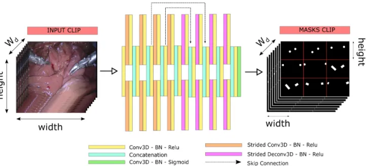
Fig. 4: Proposed network architecture. Dashed arrows refer to skip connections. Conv3D-BN-Relu: 3D convolution followed by batch normalization (BN) and rectified linear unit (Relu) activation. Strided Conv3D: 3D convolution. Strided Deconv3D: 3D deconvolution. Concatenation: joining two inputs with the same shape to assemble a unique output. Due to the impossibility to represent the 4D output (width x height x Wd x 3), where Wd is the number of frames in a temporal clip, we joined the

nine (joint+connection) masks in a single image. Input and output dimensions are reported.

B. Network architecture

To incorporate spatio-temporal information and features that are encoded in videos, we use 3D kernels with a 3 x 3 x 3 dimension for non-strided convolution [19]. The 3D con-volution allows the kernel to move along the three input dimensions to process multiple frames at the same time, preserving and processing temporal information through the network. The architecture of the proposed network is shown in Fig. 4, and Table I describes the full parameter details. The framework is similar to U-net, [20] using a modular encoder-decoder structure. We used a two-branch architecture to allow the FCNN to separately process the joint and connection masks [21]. Skip connections [20] are used in the middle layers and we employ strided convolution instead of pooling for multi-scale information propagation both up and down.

We perform a double contraction and extension of the temporal dimension by setting a kernel stride of 2 x 2 x 2 in the middle layers, between the skip connections. This con-figuration allows the model to refine the temporal information during the down-sampling (encoder) phase and recover the lost information on surgical-tool position in the up-sampling phase [22].

Each module of the network is composed of a first 3 x 3 x 3 convolutional layer that processes the input without modifying its dimension. The output is then duplicated and separately processed in the two different branches. In each branch, first a strided 3D convolution (deconvolution) is applied, halving (doubling) the spatial dimensions and the temporal dimension (only middle layers). After that, a 1 x 1 x 1 convolution is performed to double (halve) the number of image channels. Finally, the results of both branches are concatenated and processed in the next module. For every convolution, batch

normalization (BN) is applied on the output [23] and the result is processed using REctified Linear Unit (Relu) activation. A sigmoid activation function is applied after the last convolution in order to obtain the final output for the segmentation step generating image masks.

The network is trained employing Stochastic Gradient De-scend (SGD) as the optimizer, which helps the model to avoid degenerate solutions [24]. The per-pixel binary cross-entropy loss function (L) is employed for training, as suggested in [5]. L is defined as: L= 1 NΩ N X n=1 X x∈Ω [pkxlogpb k x+ (1 − pkx)log(1 −pb k x)] (1)

where N is the total number of considered masks, pkx and

b pk

x are the ground truth value and the corresponding network

output at pixel location x in the clip domain Ω of the kth

probability map.

III. EXPERIMENTS

A. Datasets

The proposed network was trained and tested using a dataset of 10 videos (EndoVis Dataset: 1840 frames, frame size = 720x576 pixels) from the EndoVis Challenge 20151. Specifically, we used 8 videos for training and 2 (EndoVis.A and EndoVis.B) for testing and validation. It is worth noticing that EndoVis.B has a completely different background with respect to the 8 training EndoVis videos, differently from EndoVis.A that has a similar background.

We further acquired 8 videos with a da Vinci Research Kit (dVRK) (UCL dVRK Dataset: 3075 frames, frame size =

(4)

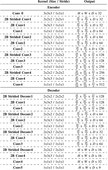
TABLE I

Specifications of the proposed network. Kernel size and stride (kernel height x kernel width x kernel depth) as well

as output dimensions (height (H) x width (W) x Wd (D) x

N◦Channels) of each layer are shown. Wd is the number of

frames that compose a temporal clip. The final output is a clip of 9 binary maps (one per joint/connection) with the

same dimension of the input.

Kernel (Size / Stride) Output Encoder Conv 0 3x3x3 / 1x1x1 Hx W x D x 32 2B Strided Conv1 2x2x2 / 2x2x1 H₂ x W₂ x D x 32 2B Conv1 3x3x3 / 1x1x1 H₂ x W₂ x D x 32 Conv1 1x1x1 / 1x1x1 H₂ x W₂ x D x 64 2B Strided Conv2 2x2x2 / 2x2x1 H₄ x W₄ x D x 64 2B Conv2 3x3x3 / 1x1x1 H₄ x W₄ x D x 64 Conv2 1x1x1 / 1x1x1 H₄ x W₄ x D x 128 2B Strided Conv3 2x2x2 / 2x2x2 H₈ x W₈ x D₂ x 128 2B Conv3 3x3x3 / 1x1x1 H₈ x W₈ x D₂ x 128 Conv3 1x1x1 / 1x1x1 H₈ x W₈ x D₂ x 256 2B Strided Conv4 2x2x2 / 2x2x2 ₁₆H x W₁₆ x D₄ x 256 2B Conv4 3x3x3 / 1x1x1 ₁₆H x W₁₆ x D₄ x 256 Conv4 1x1x1 / 1x1x1 ₁₆H x W₁₆ x D₄ x 512 Decoder 2B Strided Deconv1 2x2x2 / 2x2x2 H₈ x W₈ x D₂ x 128 2B Conv1 3x3x3 / 1x1x1 H₈ x W₈ x D₂ x 128 Conv1 1x1x1 / 1x1x1 H₈ x W₈ x D₂ x 256 2B Strided Deconv2 2x2x2 / 2x2x2 H₄ x W₄ x D x 64 2B Conv2 3x3x3 / 1x1x1 H₄ x W₄ x D x 64 Conv2 1x1x1 / 1x1x1 H₄ x W₄ x D x 128 2B Strided Deconv3 2x2x2 / 2x2x1 H₂ x W₂ x D x 32 2B Conv3 3x3x3 / 1x1x1 H₂ x W₂ x D x 32 Conv3 1x1x1 / 1x1x1 H₂ x W₂ x D x 64 2B Strided Deconv4 2x2x2 / 2x2x1 Hx W x D x 16 2B Conv4 3x3x3 / 1x1x1 Hx W x D x 16 Conv4 1x1x1 / 1x1x1 Hx W x D x 32 Conv5 1x1x1 / 1x1x1 Hx W x D x 9

720x576 pixels) to attenuate overfitting issues. In fact, with the inclusion of 3D kernels in the FCNN processing, the number of FCNN parameters increased by a factor of 3 with respect to its 2D counterpart. Seven videos were used for training/validation and one (UCL dVRK) for testing.

Dataset details, in terms of number of train-ing/validation/testing videos and frames, are reported in Table II. In Fig. 5 we show three samples from the training and test set, both from the EndoVis and UCL dVRK datasets. The UCL dVRK and EndoVis datasets were different in terms of lightning condition, background, and colour and tools.

As ground truth, we used annotations2 _{provided for the}

2_{https://github.com/surgical-vision/EndoVisPoseAnnotation}

Fig. 5: Sample images from (left and middle) EndoVis and (right) UCL dVRK datasets for (first row) training (second row) testing. The images from the two datasets are different in terms of resolution, light conditions, number of tools in the field of view, shaft shape and colour.

EndoVis dataset [5], which consisted in 1840 frames, while we manually labeled one of every three frames of the UCL dVRK dataset, resulting in 3075 annotated frames. Images were resized to 320x256 pixels in order to reduce processing time and the GPU memory requirements. For both datasets, we selected rd equal to 15 pixels.

The FCNN model was implemented in Keras3 _{and trained}

using a Nvidia GeForce GTX 1080. For training, we set an initial learning rate of 0.001 with a learning decay of 5% every five epochs and a momentum of 0.98 [25]. Following the studies carried out in [26], [27], we chose a batch size of 2 in order to improve the generalization capability of the networks. As introduced in Sec. II, our FCNN was trained using the per-pixel binary cross-entropy as loss function [5] and stochastic gradient descend as chosen optimizer. We then selected the best model as the one that minimized the loss on the validation set (∼10% of the whole dataset).

B. Conducted experiments

In Sec. III-B1 and Sec. III-B2, the two conducted experi-ments (E1 and E2) are described, respectively.

1) Experiments using different time steps (E1): We in-vestigated the network’s performance at different Ws, i.e. 4

(Step 4), 2 (Step 2) and 1 (Step 1). Inspired by [16], we always considered Wd = 8, hence obtaining 1200, 2395 and 4780 4D

data, respectively. Data augmentation was performed, flipping frames horizontally, vertically and in both the directions, hence quadrupling the amount of available data and obtaining 4800 (Step 4), 9580 (Step 2) and 19120 (Step 1) 4D data. We then trained one FCNN for each Ws.

2) Comparison with the state of the art (E2): For the comparison with the state of the art, we chose the model proposed [5], which is the most similar with respect to ours. We compared it with the model that showed the best performances according to E1.

(5)

TABLE II

Specification for the dataset used for training and testing purposes. For each video of both the Endovis and the UCL dVRK datasets, the number of frames is shown.

EndoVis Dataset: 1840 Frames (37.5% Whole Dataset)

Training Set Validation Set Test Set

Video 0 Video 1 Video 2 Video 3 Video 4 Video 5 Video 6 Video 7

Video 8 (EndoVis.A)

Video 9 (EndoVis.B) 210 Frames 300 Frames 250 Frames 80 Frames 75 Frames 75 Frames 240 Frames 75 Frames 300 Frames 235 Frames

UCL dVRK Dataset: 3075 Frames (62.5% Whole Dataset)

Training Set Validation Set Test Set

Video 0 Video 1 Video 2 Video 3 Video 4 Video 5 Video 6

Video 7 (UCL dVRK) 375 Frames 440 Frames 520 Frames 215 Frames 295 Frames 165 Frames 550 Frames 515 Frames

C. Performance metrics

For performance evaluation, inspired by similar work (e.g. [4], [5]), we compute the Dice Similarity Coefficient (DSC), Precision (Prec) and Recall (Rec):

DSC= 2T P 2T P + F N + F P (2) Prec= T P T P + F P (3) Rec= T P T P + F N (4)

where T P is the number of pixels correctly detected as joint/connection and background, while F P and F N are the number of pixels misclassified as joint/connection neighbors and background, respectively.

Multiple comparison One-Way ANOVA was performed to detect significant differences between results achieved when investigating E1 and E2, always considering a significance level (α) equal to 0.01.

For fair comparison, we selected Ws = 8 to generate the

3D test sets for both E1 and E2, as to avoid temporal-clip overlapping.

IV. RESULTS

A. E1 results

The model processing speed was on average ∼ 1 clip per second. Figure 6 shows the boxplots of the performance metrics evaluated on the three testing videos. Median DSC for Step 1, Step 2 and Step 4 were 86.1%, 85.2% and 84.8%, respectively, with InterQuartile Range (IQR) < 10% in all cases. Our analysis separately considers the performance on each of the three testing videos, obtaining the results showed in Table III. Step 1 model achieved the best results in terms of DSC and Prec on both the EndoVis.A and UCL dVRK videos (DSC=88.6%, 86.9% respectively), but showed

Fig. 6: Dice Similarity Coefficient (DSC), precision (Prec) and recall (Rec) obtained when training the proposed network with Ws = 1 (Step 1), 2 (Step 2) and 4 (Step 4).

TABLE III

Quantitative results of the proposed 3D model trained on the three datasets, using Ws= 1 (Step 1), 2 (Step 2) and 4 (Step

4). The evaluation for each of the test videos is performed in terms of median Dice similarity coefficient (DSC), precision (Prec) and recall (Rec). We highlighted in red the best scores

for every video.

Median Value of DSC(%) / Prec(%) / Rec(%) EndoVis. A EndoVis. B UCL dVRK Step 4 85.9 / 82.3 / 89.7 81.3 / 78.8 / 85.3 85.5 / 79.7 / 92.4 Step 2 86.9 / 83.2 / 91.0 83.2/80.5/86.4 85.5 / 79.4 /92.7 Step 1 88.3/85.4/91.9 80.9 / 76.0 / 86.0 86.9/82.3/ 92.4

(6)

TABLE IV

Comparison with the state of the art method proposed in [5]. Results are reported for every joint and joint-pair connection in terms of Dice similarity coefficient (DSC), precision (Prec) and recall (Rec).

Median Value of DSC(%) / Precision(%) / Recall(%)

EndoVis.A EndoVis.B UCL dVRK

Architecture 2D Architecture 3D Architecture 2D Architecture 3D Architecture 2D Architecture 3D LTP 84.0 / 81.0 / 88.8 80.9 / 76.5 / 86.6 44.6 / 36.6 / 58.7 77.6 / 82.7 / 74.7 84.7 / 83.9 / 86.5 85.7 / 83.4 / 87.6 RTP 86.0 / 83.8 / 89.9 86.7 / 87.0 / 86.6 52.3 / 39.2 / 79.0 76.4 / 73.8 / 80.4 82.4 / 78.1 / 88.7 82.0 / 75.2 / 91.3 HP 83.2 / 78.6 / 89.2 80.2 / 75.3 / 86.7 80.6 / 81.7 / 81.5 79.8 / 77.7 / 82.4 88.7 / 88.7 / 89.0 88.8 / 86.8 / 91.3 SP 89.4 / 86.3 / 93.2 86.5 / 83.1 / 92.2 81.3 / 80.2 / 82.4 82.6 / 80.3 / 84.9 91.7 / 89.7 / 94.1 90.3 / 86.8 / 93.5 EP 86.1 / 84.4 / 90.4 86.6 / 86.0 / 87.7 88.0 / 90.0 / 89.3 89.1 / 86.6 / 92.7 58.3 / 42.9 / 91.8 74.0 / 63.5 / 90.2 LTP-HP 88.1 / 86.1 / 90.9 87.7 / 82.9 / 93.2 50.5 / 36.4 / 84.5 81.4 / 76.5 / 88.3 89.0 / 86.8 / 90.9 88.8 / 84.8 / 93.5 RTP-HP 89.3 / 85.9 / 94.5 89.2 / 87.1 / 92.4 45.2 / 29.8 / 92.3 81.3 / 80.8 / 83.1 89.7 / 89.7 / 90.6 88.9 / 85.4 / 93.3 HP-SP 90.1 / 87.7 / 92.1 87.7 / 83.4 / 93.9 78.5 / 74.2 / 83.8 81.7 / 75.1 / 88.8 91.3 / 89.7 / 93.3 89.6 / 85.3 / 94.8 SP-EP 91.1 / 88.5 / 93.5 90.7 / 87.7 / 93.8 91.0 / 88.7 / 93.7 90.9 / 87.2 / 95.4 82.4 / 71.8 / 97.6 87.4 / 80.0 / 96.8

Fig. 7: Visual examples of (left) ground-truth segmentation, and segmentation outcomes obtained with (center) the network proposed in [5], and (right) the proposed network for the UCL dVRK dataset. Red arrows highlight regions misclassified as joint or connection.

TABLE V

First experiment (E1) One-Way Anova test results.

DSC F(2, 429) = 16.85 p-value < 0.01 F(2, 693) = 14.33 p-value < 0.01 F(2, 1533) = 32.73 p-value < 0.01 Prec F(2, 429) = 15.49 p-value < 0.01 F(2, 693) = 24.59 p-value < 0.01 F(2, 1553) = 84.56 p-value < 0.01 Rec F(2, 429) = 9.1 p-value < 0.01 F(2, 693) = 4.35 p-value = 0.013 F(2, 1553) = 3.9 p-value = 0.02

the worst performances on EndoVis.B (DSC=80.9%). Step 2 model obtained the highest scores in all the metrics of EndoVis.B, while Step 4 showed the lowest performance in all the three test videos. One-Way Anova test always highlighted significant differences except for EndoVis.B and UCL dVRK Rec, as shown in Table V.

Since EndoVis.B presented the most challenging

back-Fig. 8: Visual examples of (left) ground-truth segmentation, and segmentation outcomes obtained with (center) the network proposed in [5], and (right) the proposed network, for the EndoVis.B dataset. Red arrows highlight regions misclassified as joint or connection.

ground, we selected Step 2 dataset to train our model in the successive experiment.

B. E2 results

Table IV shows the results achieved by the proposed model in comparison with [5], while VI show the same results

(7)

TABLE VI

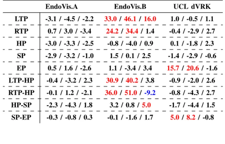
Comparison with the state of the art method proposed in [5]. Results are reported in terms of difference between the

proposed and state-of-the-art median values of Dice similarity coefficient (DSC), precision (Prec) and recall

(Rec). We highlighted in red (positive values) and blue (negative values) the scores where the two models achieved

substantially different results (≥ ±5%)

∆ Median Value of DSC(%) / Prec(%) / Rec(%)

LTP -3.1 / -4.5 / -2.2 33.0/46.1/16.0 1.0 / -0.5 / 1.1 RTP 0.7 / 3.0 / -3.4 24.2/34.4/ 1.4 -0.4 / -2.9 / 2.7 HP -3.0 / -3.3 / -2.5 -0.8 / -4.0 / 0.9 0.1 / -1.8 / 2.3 SP -2.9 / -3.2 / -1.0 1.5 / 0.1 / 2.5 -1.4 / -2.9 / -0.6 EP 0.5 / 1.6 / -2.6 1.1 / -3.4 / 3.4 15.7/20.6/ -1.6 LTP-HP -0.4 / -3.2 / 2.3 30.9/40.2/ 3.8 -0.9 / -2.0 / 2.6 RTP-HP -0.1 / 1.2 / -2.1 36.0/51.0/-9.2 -0.8 / -4.3 / 2.7 HP-SP -2.3 / -4.3 / 1.8 3.2 / 0.8 /5.0 -1.7 / -4.4 / 1.5 SP-EP -0.3 / -0.8 / 0.3 -0.1 / -1.6 / 1.7 5.0/8.2/ -0.8 TABLE VII

One-Way Anova test results for E2.

DSC F(1, 286) = 8.21 p-value < 0.01 F(1, 462) = 1031.26 p-value < 0.01 F(1, 1022) = 35.56 p-value < 0.01 Prec F(1, 286) = 19.33 p-value < 0.01 F(1, 462) = 2028.31 p-value < 0.01 F(1, 1022) = 38.94 p-value < 0.01 Rec F(1, 286) = 0.09 p-value = 0.76 F(1, 462) = 13.86 p-value < 0.01 F(1, 1022) = 18.32 p-value < 0.01

in terms of difference between the two models. The differ-ences (∆) of the median performance metrics obtained by the proposed Step 2 FCNN and the one proposed in [5] are shown for each joint and connection (e.g. for LTP, results are reported as ∆DSC(LTP) = DSC3D(LTP) - DSC2D(LTP)).

When considering the UCL dVRK testing video, the pro-posed FCNN substantially outperformed the state of the art on EP and SP-EP, achieving ∆DSC differences of +15.7% and +5.0%. A sample of the performed segmentation for the two models is shown in Fig. 7 for EP and SP-EP for illustration purposes.

Finally, the proposed model outperformed [5] on LTP, RTP, LTP-HP and RTP-HP on EndoVis.B, showing improvements on ∆DSC of +33%, +24.2%, +30.9% and +36.0% respectively, while achieving one lower value only for Rec value of RTP-HP connection. Considering the performances on the whole test set, the proposed model achieved a median DSC score of 85.1% with IQR=4.6%. Visual segmentation examples are shown in Fig. 8. One-Way Anova Test did not show significant similarities, except for EndoVis.A Rec, as shown in Table VII.

V. DISCUSSION

A. E1 discussion

The results we obtained on EndoVis.A and UCL dVRK may be explained considering that the backgrounds in the videos are very similar to the ones of the videos of the training set, meanwhile EndoVis.B’s background is completely missing in the training data domain. The low DSC score achieved by Step 1 model on EndoVis.B, coupled with the high scores on the other two datasets, showed that, with high probability, the model overfitted. Such a conclusion may be expected: despite the large amount of data, the high correlation between datasets, due to the use of a temporal step Ws of only one frame, led

the sliding window algorithm to produce a dataset with too little variability for training a model over a good domain.

The model trained on Step 4 dataset was not able to achieve competitive results in any of the test videos with respect to the other models. Since the proposed architecture has a very large number of parameters (∼ 80000), it needs a huge amount of data in order to be properly trained. For this reason, the model achieves lower quality predictions.

The network trained on Step 2 dataset achieved the best scores for all the considered metrics on EndoVis.B. This may be explained as Ws=2 strikes a balance between the

amount of data and the similarity between the frames. We select this model for the successive comparison with the architecture presented in [5], due to its capability to generalize on backgrounds not already seen in the training phase. B. E2 discussion

EndoVis.A was probably the less challenging video in terms of background complexity and both the proposed and network showed similar results [5]. When instead the EndoVis.B test video was considered, the previous model [5] was barely able to properly recognize and separate tip joints and connections from the background, achieving poor DSC values and over-estimating joint/connection detection. This result is visible in Fig. 8, where multiple tip-points are erroneously detected for LTP and RTP and double connections for the related joint pairs.

On the other hand, the results obtained by the 3D network suggest that the temporal information was exploited to improve the network generalization capability on unseen backgrounds, obtaining DSC scores of 77.6% and 76.4% for LTP and RTP, respectively, as shown in Table IV.

Similarly, the testing performance achieved on the UCL dVRK dataset by the proposed 3D model outperformed that achieved by [5]. In fact, as shown in Fig. 7, the background presented homogeneous portions in terms of texture and color that were misclaissified as EP when not including temporal information, while the proposed 3D model showed its ability to better separate joints and joint-pair connections from back-ground, achieving a ∆DSC of +15.7% and +5.0% on EP and SP-EP, respectively.

C. Limitations and future work

An obvious limitation of this study is the limited number of testing videos, which is due to the lack of available annotated

(8)

data. Nonetheless, this number is comparable to that of similar work in the literature [5] and we will release the data we collected for further use in the community. As future work, it would be interesting to assess the model performance when varying Wd. Moreover, a larger test set, which will possibly

encode challenges such as smoke and occlusions, should be collected, annotated and analyzed, too.

A second issue is related to the 2D nature of the esti-mated joint position. It would be interesting to include da Vinci (Intuitive Surgical Inc, CA) kinematic data in theR

joint/connection position estimation. Such information may be useful to provide a more robust solution for occluded joints. This is realistic and feasible using dVRK information but requires careful calibration and data management. While dVRK encoders are able to provide kinematic data for end-effector 3D position and angles between robotic-joint axes, this requires a projection on the image plane to be suitable for 2D tracking, with errors associated to encoders’ precision.

Natural extensions of the proposed work would be to include the instrument articulation estimation within other scene understanding algorithms, e.g. computational stereo or semantic SLAM, in order help with algorithms coping with the boundary regions between instruments and tissue.

VI. CONCLUSION

In this paper, we proposed a 3D FCNN architecture for surgical-instrument joint and joint-connection detection in MIS videos. Our results, achieved by testing existing datasets and new contribution datasets, suggest that spatio-temporal features can be successfully exploited to increase segmentation performance with respect to 2D models based on single-frame information for surgical-tool joint and connection detection. This moves us towards a better framework for surgical scene understanding and can lead to applications of CAI in both robotic systems and in surgical data science.

ACKNOWLEDGEMENTS

This work was supported by the Wellcome/EPSRC Centre for Interventional and Surgical Sciences (WEISS) at UCL (203145Z/16/Z) and EPSRC (EP/N027078/1, EP/P012841/1, EP/P027938/1, EP/R004080/1).

REFERENCES

[1] J. H. Palep, “Robotic assisted minimally invasive surgery,” Journal of Minimal Access Surgery, vol. 5, no. 1, pp. 1–7, 2009.

[2] H. Azimian, R. V. Patel, and M. D. Naish, “On constrained manipulation in robotics-assisted minimally invasive surgery,” in IEEE RAS & EMBS International Conference on Biomedical Robotics and Biomechatronics. IEEE, 2010, pp. 650–655.

[3] S. Moccia, S. J. Wirkert, H. Kenngott, A. S. Vemuri, M. Apitz, B. Mayer, E. De Momi, L. S. Mattos, and L. Maier-Hein, “Uncertainty-aware organ classification for surgical data science applications in laparoscopy,” IEEE Transactions on Biomedical Engineering, vol. 65, no. 11, pp. 2649– 2659, 2018.

[4] S. Moccia, S. Foti, A. Routray, F. Prudente, A. Perin, R. F. Sekula, L. S. Mattos, J. R. Balzer, W. Fellows-Mayle, E. De Momi et al., “Toward improving safety in neurosurgery with an active handheld instrument,” Annals of Biomedical Engineering, vol. 46, no. 10, pp. 1450–1464, 2018. [5] X. Du, T. Kurmann, P.-L. Chang, M. Allan, S. Ourselin, R. Sznitman, J. D. Kelly, and D. Stoyanov, “Articulated multi-instrument 2-D pose estimation using fully convolutional networks,” IEEE Transactions on Medical Imaging, vol. 37, no. 5, pp. 1276–1287, 2018.

[6] M. Allan, S. Ourselin, D. J. Hawkes, J. D. Kelly, and D. Stoyanov, “3-D pose estimation of articulated instruments in robotic minimally invasive surgery,” IEEE Transactions on Medical Imaging, vol. 37, no. 5, pp. 1204–1213, 2018.

[7] T. Kurmann, P. M. Neila, X. Du, P. Fua, D. Stoyanov, S. Wolf, and R. Sznitman, “Simultaneous recognition and pose estimation of instruments in minimally invasive surgery,” in International Conference on Medical Image Computing and Computer-Assisted Intervention. Springer, 2017, pp. 505–513.

[8] M. Allan, A. Shvets, T. Kurmann, Z. Zhang, R. Duggal, Y.-H. Su, N. Rieke, I. Laina, N. Kalavakonda, S. Bodenstedt et al., “2017 Robotic instrument segmentation challenge,” arXiv preprint arXiv:1902.06426, 2019.

[9] M. Groeger, K. Arbter, and G. Hirzinger, “Motion tracking for minimally invasive robotic surgery,” in Medical Robotics. IntechOpen, 2008. [10] A. Krupa, J. Gangloff, C. Doignon, M. F. De Mathelin, G. Morel,

J. Leroy, L. Soler, and J. Marescaux, “Autonomous 3-D positioning of surgical instruments in robotized laparoscopic surgery using visual servoing,” IEEE Transactions on Robotics and Automation, vol. 19, no. 5, pp. 842–853, 2003.

[11] R. Sznitman, C. Becker, and P. Fua, “Fast part-based classification for instrument detection in minimally invasive surgery,” in International Conference on Medical Image Computing and Computer-Assisted In-tervention. Springer, 2014, pp. 692–699.

[12] S. Bodenstedt, M. Allan, A. Agustinos, X. Du, L. Garcia-Peraza-Herrera, H. Kenngott, T. Kurmann, B. M¨uller-Stich, S. Ourselin, D. Pakhomov et al., “Comparative evaluation of instrument segmentation and tracking methods in minimally invasive surgery,” arXiv preprint arXiv:1805.02475, 2018.

[13] S. Kumar, M. S. Narayanan, P. Singhal, J. J. Corso, and V. Krovi, “Product of tracking experts for visual tracking of surgical tools,” in IEEE International Conference on Automation Science and Engineering. IEEE, 2013, pp. 480–485.

[14] A. A. Shvets, A. Rakhlin, A. A. Kalinin, and V. I. Iglovikov, “Automatic instrument segmentation in robot-assisted surgery using deep learning,” in 2018 17th IEEE International Conference on Machine Learning and Applications (ICMLA). IEEE, 2018, pp. 624–628.

[15] Z. Zhao, Z. Chen, S. Voros, and X. Cheng, “Real-time tracking of sur-gical instruments based on spatio-temporal context and deep learning,” Computer Assisted Surgery, pp. 1–10, 2019.

[16] R. Hou, C. Chen, and M. Shah, “An end-to-end 3D convolutional neural network for action detection and segmentation in videos,” arXiv preprint arXiv:1712.01111, 2017.

[17] D. Maturana and S. Scherer, “Voxnet: A 3D convolutional neural network for real-time object recognition,” in IEEE/RSJ International Conference on Intelligent Robots and Systems.

[18] I. Funke, S. T. Mees, J. Weitz, and S. Speidel, “Video-based surgical skill assessment using 3D convolutional neural networks,” arXiv preprint arXiv:1903.02306, 2019.

[19] D. Tran, L. Bourdev, R. Fergus, L. Torresani, and M. Paluri, “Learning spatiotemporal features with 3D convolutional networks,” in IEEE International Conference on Computer Vision, 2015, pp. 4489–4497. [20] O. Ronneberger, P. Fischer, and T. Brox, “U-net: Convolutional

net-works for biomedical image segmentation,” in International Conference on Medical Image Computing and Computer-Assisted Intervention. Springer, 2015, pp. 234–241.

[21] Z. Cao, T. Simon, S.-E. Wei, and Y. Sheikh, “Realtime multi-person 2D pose estimation using part affinity fields,” in Conference on Computer Vision and Pattern Recognition, 2017, pp. 7291–7299.

[22] X. Mao, C. Shen, and Y.-B. Yang, “Image restoration using very deep convolutional encoder-decoder networks with symmetric skip connec-tions,” in Advances in Neural Information Processing Systems, 2016, pp. 2802–2810.

[23] S. Ioffe and C. Szegedy, “Batch normalization: Accelerating deep network training by reducing internal covariate shift,” in International Conference on Machine Learning, 2015, pp. 448–456.

[24] S. Mandt, M. D. Hoffman, and D. M. Blei, “Stochastic gradient descent as approximate bayesian inference,” The Journal of Machine Learning Research, vol. 18, no. 1, pp. 4873–4907, 2017.

[25] M. D. Zeiler, “Adadelta: an adaptive learning rate method,” arXiv preprint arXiv:1212.5701, 2012.

[26] N. S. Keskar, D. Mudigere, J. Nocedal, M. Smelyanskiy, and P. T. P. Tang, “On large-batch training for deep learning: Generalization gap and sharp minima,” arXiv preprint arXiv:1609.04836, 2016.

[27] D. Masters and C. Luschi, “Revisiting small batch training for deep neural networks,” arXiv preprint arXiv:1804.07612, 2018.