”Sapienza” University of Rome
Protein Sequencing Strategy in
NanoTechnology by Classical and
Quantum Atomistic Models
XXXI
Ph.D. student:
Aldo Eugenio Rossini
Mathematical Models for Engineering, Electromagnetics and
Nanosciences
Contents
Introduction 1
1 State of the Art 3
1.1 Nanopore Sensing . . . 3
1.1.1 Biological Nanopores . . . 5
Alpha-Hemolysin . . . 5
1.1.2 Solid-State Nanopores . . . 7
Graphene . . . 8
1.2 Nanopore for Bio-Molecules . . . 10
Polynucleotides . . . 10
Proteins . . . 12
1.2.1 DNA Sequencing . . . 13
1.2.2 Proteins and Peptides Sequencing . . . 16
1.3 Atomistic Approaches to Nanopore . . . 20
2 Theoretical Methods 21 2.1 Molecular Dynamics . . . 21
2.1.1 Steered Molecular Dynamics . . . 22
Ionic Current . . . 24
2.2 Density Functional Theory . . . 25
The Hohenberg-Kohn Theorems . . . 26
The Kohn-Sham Theory . . . 27
The Exchange-Correlation Functionals . . . 28
Pseudopotentials . . . 29
2.3 Quantum Transport Theory . . . 31
2.3.1 Elastic Transport . . . 32
Non-Equilibrium Green’s Function and Landauer-Büttiker Formula . . . 35
2.3.2 Inelastic Condutance . . . 38
CONTENTS CONTENTS 3 Atomistic Modelling 44
3.1 Classical Molecular Dynamics . . . 44
Molecular Dynamics with NAMD . . . 44
3.1.1 System Chosen . . . 45
Device and Target . . . 45
3.1.2 Simulation Set-Up . . . 47
3.2 Quantum Molecular Dynamics . . . 50
DFT in TranSIESTA . . . 50
3.2.1 System Chosen . . . 51
Device and Target . . . 52
3.2.2 Simulation Set-Up . . . 54
4 Results and Discussion 58 4.1 Current Blockage . . . 58 4.2 Elastic Signal . . . 65 Glycine homo-peptide . . . 65 Hetero-peptides . . . 72 4.3 Inelastic Signal . . . 76 5 Conclusion 78 5.1 Classical Molecular Dynamics . . . 78
5.2 Quantum Molecular Dynamics . . . 79
A Appendices 80 A.1 NAMD . . . 80 A.2 VMD . . . 81 A.3 CHARMM . . . 82 A.4 SIESTA . . . 84 A.5 TranSIESTA . . . 86 A.6 INELASTICA . . . 88
A.7 Quantum ESPRESSO . . . 89
List of Figures
1 Nanopore Sensing . . . 2
1.1 Nanopore Working Principle . . . 4
1.2 Channel Alpha-Hemolysin . . . 6
1.3 Sites Alpha-Hemolysin . . . 7
1.4 Solid-State Nanopore . . . 8
1.5 Nanopore Architectures Terrace . . . 9
1.6 Conformation of DNA . . . 12
1.7 Structure of Amino acids . . . 13
1.8 First and Second Generation of DNA Sequencing . . . 14
1.9 The Sequencing Technique of Oxford Nanopore Technologies . 15 1.10 Schematic Transit Protein in Pore . . . 16
1.11 Protein in Nanopore . . . 18
1.12 Protein in Sequencing . . . 19
2.1 Steered Molecular Dynamics . . . 23
2.2 Molecular Dynamics . . . 24
2.3 Pseudopotential . . . 30
2.4 The Resistance of a Conductor . . . 31
2.5 Elastic Transport Scheme . . . 33
2.6 Current-Voltage Scheme . . . 34 2.7 NEGF Zone . . . 35 2.8 NEGF Scheme . . . 36 2.9 NEGF Formalism . . . 39 2.10 LOE vs LOE-WBA . . . 41 2.11 IETS Mechanisms . . . 43
3.1 System Chosen for Classical Molecular Dynamics . . . 46
3.2 Peptide translocation via molecular dynamics simulation . . . 48
3.3 Student’s T-test adjusted p-value matrix . . . 49
3.4 Graphene Nanopore . . . 51
LIST OF FIGURES LIST OF FIGURES
3.6 Idea Device . . . 53
3.7 Transmission function of the hydrated ZGNR . . . 54
3.8 Set-Up . . . 54
3.9 Transmission function of ZGNR - Ammino Acids . . . 57
4.1 Ionic current measurements . . . 59
4.2 Ionic current measurements . . . 60
4.3 Accessible volume and correlation with measured currents . . 61
4.4 Pore clogging . . . 63
4.5 ↵Hemolisine truncated . . . 64
4.6 Glycine . . . 65
4.7 Electron current Glycine . . . 66
4.8 Transmission coefficients for Glycine . . . 67
4.9 PDOS for Glycine . . . 68
4.10 Bond current for Glycine . . . 69
4.11 Side-Chain Glycine . . . 71
4.12 Electron current Alanine . . . 73
4.13 Electron current Asparagine . . . 74
4.14 Electron current Asparagine . . . 75
4.15 Inelastic current . . . 76
4.16 Phonon-DOS for the Glycine groups . . . 77
4.17 IETS for the Glycine groups . . . 77
A.1 Internal coordinates for bonded interactons . . . 84
Introduction
This thesis focuses on simulations for peptides sequencing, based on the Nanopore technology. Nanopore sensing is a single-molecule technique ca-pable of detecting peptide and protein by monitoring the change in current generated by the interaction of protein with nanopore devices. To better un-derstand what happens in the nanopore devices, we analyze them by means of two methods: one classical to study the ionic current and take an overview of the phenomena with the possibility of simulating more atoms; and one quantum to study the tunneling current and have a more precise signal.
For the classical model, the idea of using nanopores inserted in lipid mem-branes, as a tool for the analysis of single molecules, was inspired by the very intense molecular transport activity between the intracellular and the ex-tracellular media as well as between different cellular organelles. Molecular transport across the naturally impermeable membranous structures of cells occurs through a variety of protein channels incorporated into the fluid mo-saic of the lipid bilayers. These channels or pores act as gates through which a wide variety of molecules such as ions, sugars, nucleic acids and proteins can pass during their transport from one organelle to another, or from the cytoplasm to the outside of the cell. The ability of the pores to allow the passage of ions and larger molecules suggested that the ions could be used to carry an electric current, which in turn could drive larger polar molecules through the channels. The change in the ionic flow through the channel due to the transit of the macromolecule could depend on the structure of the particular translocating molecule.
The quantum study focuses on the ab-initio simulations of charge trans-port through nano-gap of graphene. The Latin word ab-initio ("from begin-ning") means that no adjustable parameters are needed in the simulation. An atomistic description of materials and nanosystems without fitting parame-ters has an unprecedented predictive power for the study of their physical properties and gives access to an extremely broad range of phenomena oth-erwise not observable. The ab-initio simulations applied for charge transport mechanisms have recently emerged in both pure and applied research, as a
Introduction powerful technique to gain insight into the quantum phenomena governing the conduction properties of systems with reduced dimensionality where clas-sical charge transport models are no longer valid. One of the most widely used techniques for the ab-initio calculation of the electronic transport prop-erties is based on the combination of density functional theory (DFT) for the electronic structure with the non-equilibrium Green’s function (NEGF) for quantum transport.
But why do we bother studying into these new sequencing techniques? The first attempt to sequencing the human genome was started in 1990 by the US government under the name of the ’Human Genome Project’. This project was successfully completed in the year 2003, with a cost of about $ 2.7 billion; at that time, the so-called Sanger method [1] was used, now the DNA sequencing is carried out with nanopore devices 1 [2]. After DNA sequencing was born "Human proteome project" for the sequencing of pro-teins. The recents progresses in biology have allowed to select amino-acid sequences; but sequencing of amino-acid chains (peptides, proteins) in an effective manner (rapid, selective) is not possible yet. The importance of identifying the sequence and the structure of proteins and polypeptides is crucial, because mis-folding of proteins (structured and not), is believed to be related to neurodegenerative diseases such as Parkinson’s and Alzheimer [3] as well as the post-translational modifications [4]. In order to achieve a better understanding of genetics, mutations, it is vital to have a low-cost, highly parallelizable way of sequencing. This could lead to so-called personal-ized medicine, meaning that it would be affordable for a person to have their genome sequenced in order to find potential weaknesses or predispositions for certain illnesses.
Figure 1: Illustration of a single-stranded DNA molecule passing through ↵HL nanopore [2].
Chapter 1
State of the Art
Initially intended as a tool for DNA and RNA analysis with the long term goal of rapid nucleic acid sequencing, the method of sensing with nanopores was later extended for investigating a broad spectrum of molecules ranging from metal ions, small organic compunds and short peptides to chemical warfare agents, proteins and bio-molecular complexes. In this chapter, the most sig-nificant advances in nucleic acid as well as in peptide and protein detection with nanopores will be presented.
1.1 Nanopore Sensing
The idea of using nanopores inserted in lipid membranes as a tool for the anal-ysis of single molecules was inspired by the very intense molecular transport activity between the intracellular and the extracellular media as well as be-tween different cellular organelles. Molecular transport across the naturally-impermeable membranous structures of cells occurs through a variety of pro-tein channels incorporated into the fluid mosaic of the lipid bilayers. These channels or pores act as gates through which a wide variety of molecules such as ions, sugars, nucleic acids and proteins can pass during their transport from one organelle to another, or from the cytoplasm to the outside of the cell. The ability of the pores to allow the passage of ions and larger molecules sug-gested that the ions could be used to carry an electric current which in turn could drive larger polar molecules through the channels. The change in the ionic flow through the channel due to the transit of the macromolecule would depend on the structure of the particular translocating molecule. Similar to the natural molecular translocation mechanism through protein channels, the nanopore detection method utilizes a nanopore inserted into an insulating membrane separating two chambers filled with a buffer/electrolyte solution.
Nanopore Sensing State of the Art The principle for nanopore detection is similar to the Coulter counter used for counting and sizing particles [5]. An electric potential is applied across the membrane via two electrodes and the ionic current through the open pore is monitored. When a charged molecule is driven into and through the nanopore by the electric potential, it causes a drop in the ionic current. The ionic current drop has a characteristic amplitude (Iblock) and duration (Tblock)
reflecting the particular structure of that molecule (Fig. 1.1). The ampli-tudes are related to the volume of the molecule while the durations depend mainly on its length and charge; the changes in the volume and length of the molecule are connected to the particular structure adopted in solution. Thus, in principle, nanopore detection could be used to distinguish between iden-tical molecules adopting different conformations. This feature could prove useful for the investigation of protein mis-folding diseases.
Figure 1.1: Current through the nanopore device attracts the target in the pore. The nanometer pore allows the analysis to single molecule. During translocation the output signal changes allowing to analyze the target.
Currently, there are two types of pores used for the nanopore detection method: protein pores and solid-state pores. The protein pores belong to the group of pore-forming toxins produced by bacteria with damaging effects on the cytoplasmic phospholipid bilayer of human and animal cells. Their innate property of auto-insertion into lipid bilayers played a crucial part in establishing this group of proteins as sensors. Solid-state pores have been developed with the goal of improving the life span of the nanopore setup by using synthetic membranes, the range of molecules that can be analyzed by controlling the pore diameter as well as the range of experimental conditions that can be used (pH, temperature, ionic strength, applied potentials, etc.).
Nanopore Sensing State of the Art
1.1.1 Biological Nanopores
The biological nanopores possess numerous advantages which make them good targets for experimental and computational research. Firstly, their atomistic structures are usually known from X-ray crystallographic studies. Secondly, their properties may be altered through the relatively simple means of site-directed mutagenesis; it is possible not only to mutate a residue, but also to alter its properties further by coupling an additional molecule to the pore via. The heterogeneity observed among biological nanopores in terms of size and composition; the cells can produce large numbers of biological nanopores with an atomic level of precision that can not yet be replicated by the artificially.
Alpha-Hemolysin
The biological nanopores traditionally used is the heptameric protein ↵-Hemolysin. ↵-Hemolysin is a nanopore from the bacteria that causes lysis of red blood cells; its pore is a channel-protein 10 nm long with two distinct 5 nm sections made of 3.6 nm diameter vestibule connected to a transmem-brane -Barrel that is 2.6 nm wide. The very important particular is that the size vestibule is just 1.4 nm wide, which means that single-stranded DNA can pass through the nanopore, but double-stranded DNA cannot (Fig. 1.2), suggesting the potential emergence of ↵-Hemolysin as a next-generation se-quencing tool.
The problem that the molecules move through the nanopore at high ve-locities (for the DNA estimated to be 1 nucleotide per microsecond) under typical experimental conditions. These velocities mean that only a small number of ions (as few as 100) are available in the nanopore to correctly identify any given nucleotide, so the small changes in the ionic current due to the presence of different nucleotides are likely to be overwhelmed by ther-modynamic fluctuations. Sequencing using ↵-Hemolysin has been developed through basic study and structural mutations, an approaches typical is to incorporate enzymes to regulate the transport. An enzyme coupled to a nanopore is attractive for two reasons:
• The enzyme helping to capturing electrophoretically in the nanopore the molecule in solution.
• The motion is slowed and controlled from as the enzyme processes the molecules.
A example of mutation of the protein ↵-Hemolysin that improves the de-tection abilities of the pore [6] is binding of an exonuclease onto the pore.
Nanopore Sensing State of the Art
Figure 1.2: A cross-section of the heptameric transmembrane form of ↵-Hemolysin. The diameters of the pore features are as follows: cis-entrance, 28 Å; inner chamber, 46 Å; constriction, 14 Å; transmembrane barrel, about 20 Å; trans-entrance, 24 Å. The height of the entire pore is about 100 Å, while the con-striction to the trans-entrance measures about 52 Å. Residues of particular interest are also highlighted.
The enzyme cleaves the single bases, enabling the pore to identify succes-sive bases. Coupling an exonuclease to the biological pore would slow the translocation of the DNA through the pore, and increase the accuracy of data acquisition. Also recents studies have pointed to the ability of ↵-Hemolysin to detect nucleotides at two separate sites in the lower half of the pore [7]. The R1 and R2 sites (Fig. 1.3) enable each base to be monitored twice as it moves through the pore.
This method improves single reading through the nanopore by doubling the sites where the sequence is read by nanopore. Although ↵-Hemolysin has dominated the biological nanopore sequencing landscape so far, other more efficient biological nanopores are emerging. A structural drawback with ↵-Hemolysin is that the cylindrical -Barrel can accommodate up to 10 nucleotides at a time, all significantly modulate the current into pore [8]; this dilutes the ionic signature of the single nucleotide in the 1.4 nm constriction, thus reducing the overall signal-to-noise ratio in sequencing applications; to solve this problem, it was estimated to truncate the -Barrel up to the con-striction [9].
Nanopore Sensing State of the Art
Figure 1.3: Schematic representation of an oligonucleotide (blue) immobilized inside an ↵-Hemolysin pore (grey) by the use of a biotin (yellow) streptavidin (red). The ↵-Hemolysin pore can be divided into two halves, each approximately 5 nm in length containing a roughly spherical vestibule, the transmembrane -Barrel, within this is located the constriction 1.4 nm diameter (green). R1, R2, and R3 represent the three base-recognition sites in the ↵-Hemolysin nanopore within the -Barrel domain of the pore.
1.1.2 Solid-State Nanopores
Synthetic nanopores present several advantages of relevance for the biotech-nological application sensing and sequencing. Firstly, they have the potential to be significantly more robust than protein nanopores, which may be de-stroyed or disrupted by high transmembrane potentials and extremes of pH and temperature. One can envisage such robustness being of tremendous value when applied to large scale sequencing. Not being limited to biological molecules, synthetic nanopores may be constructed from a wider variety of materials. The solid-state approach offers the ability to regulate not only the size but also the nanopore shape, with a sub-nanometre precision the ability to fabricate high-density arrays of nanopores, superior mechanical, chemical and thermal characteristics and the possibility of integrating with electronic readout techniques. This can grant them interesting properties such as elec-trical conductance, which, for example, allows elecelec-trical measurements to be made directly at the pore.
Nanopore Sensing State of the Art There has been considerable progress in engineering and harnessing syn-thetic nanopores over the past decade. The first sculpting of synsyn-thetic nanopores from thin solid-state membranes of Si3N4 with highly focused
low-energy ion beams [10]; the pores fabricated with this method were asym-metrical in terms of geometry and electrical properties. Other groups [11, 12] prefer to use a electron beam with a diameter probe of few nanometres [13], these solid-state nanopore are able to selectively analize segments of single stranded DNA across the pore [14]; a major advantage of this technique is that direct visual feedback is possible through the TEM which allows con-trolling the pore diameter with single nanometer precision. Recently, 1-5 nm thick graphene membranes electron-beam sculpted nanopore have been developed (Fig. 1.4 a).
Figure 1.4: Solid-statenanopores fabricated with two-dimensional nanomem-branes: a a graphene nanopore; b a BN nanopore; c a MoS2 nanopore; [15–17].
Graphene
Graphene is a two-dimensional sheet of carbon atoms; it possesses remarkable mechanical, electrical and thermal properties. Moreover, the thickness of a single layer of graphene is comparable to the space between nucleotides inside the DNA (0.32-0.52 nm), making it particularly attractive for single-molecule sequencing [18]. In 2008 have been fabricated the first nanopores in
Nanopore Sensing State of the Art graphene films and subsequent transmission electron microscopy (TEM) the following studies elucidated the kinetics of pore formation, stability of the pore in graphene and how to detect single DNA molecules using nanopores in graphene films; the films are prepared either by chemical vapor deposition or exfoliation from graphite and the nanopores (diameters 2-25 nm) were produced by a focused electron beam [19]. It was found for graphene that the conductance of the nanopore was proportional to the pore diameter, whereas the conductance is typically proportional to the square of the diameter for SixNy but it is much thicker [15]. They also found that the conductance
for a given diameter of nanopore remained largely constant as the number of graphene layers in the membrane was increased from one to eight. So it is possible to produce a multilayer graphene nanopore, with the number of layers increasing as we move away from the pore (Fig. 1.5).
Figure 1.5: TEM image of a terraced nanopore formed in a graphene film con-taining 10 monolayers of carbon atoms. Scale bar, 1 nm. Bottom left: nanopore in a monolayer of graphene with primarily armchair edges surrounded by multilayered regions. Scale bar, 1 nm. Bottom right: TEM image of a nanopore in multilayer graphene; ripples at the pore edge again show the terraced structure.
This conformation "terraced" was confirmed using TEM image analy-sis [20]; a terraced nanopore architecture could prove very useful for many reasons, kind multilayered support may increase the stability and longevity of a graphene nanopore sensor. The terraced effect gives induced greater current blockades than the nanopores in single-layer graphene under normal conditions. The first computer simulations with the DNA passing through a graphene nanopore revealed a resolution similar to the size of an individ-ual nucleotide. This result suggests that should be possible single-nucleotide detection with an electronic read.
Nanopore for Bio-Molecules State of the Art
1.2 Nanopore for Bio-Molecules
Knowledge of the bio-molecule sequence represents an opportunity onto which a broad range of biological phenomena can be studied. Over the past years, more devices for DNA sequencing have become widely available, reducing the cost, and the possibility to put the sequencing capacity of a major genome center in the hands of individual investigators. These new technologies are rapidly evolving, and near-term challenges include the development of ro-bust protocols for generating sequencing libraries, building effective new ap-proaches to data analysis and new experimental designs. Next-generation molecules sequencing has the potential to dramatically accelerate bio-logical and biomedical research, by enabling the comprehensive analysis of genomes. Nanopores are seen as a potential next-generation sequencer that could provide cheap and fast sequencing. A crucial problem to the success of nanopores as a reliable analysis tool is the fast and stochastic nature of the bio-molecules translocation. It searches with studies experimental new mod-ifications for slowing and controlling the translocation, such has the incor-poration of biological motors. The most studied biomolecules with nanopore systems are polynucleotides and proteins.
Polynucleotides
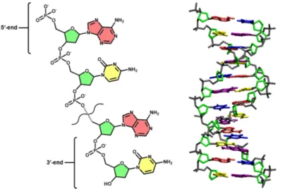
Polynucleotides in nature exist in two classes: deoxyribonucleic acid (DNA) or ribonucleic acid (RNA). DNA stores genetic information for the devel-opment and function of living organisms and some viruses. RNA is tran-scribed from DNA by enzymes in the production of proteins, and most viruses keep their genetic information in the form of RNA. The molecular structure of DNA is shown on the left of F igure 1.6. Each nucleotide monomer in the polymeric chain is composed of a nucleotide base, a pentose sugar (de-oxyribose), and a phosphate group [21]. The deoxyribose sugar and phos-phate group form the repeat unit of the polynucleotide backbone, with each monomer connecting to the one via a phosphodiester bond. At physiolog-ical pH, the phosphate groups in the polynucleotide chain possess a single negative charge while terminal phosphate groups posses a double negative charge. The terminus that ends with a phosphate group is called the 5’-end due to the relation to the pentose sugar. The opposite end, which is ter-minated at a pentose sugar, is termed the 3’-end. Attached to the pentose sugar is one of four types of nucleotide base: cytosine, guanine, adenine and thymine. These nucleotide bases can form hydrogen bonds to complementary bases. This interaction is specific due to the matching molecular structures and hydrogen bonding pattern between guanine and cytosine, or adenine and
Nanopore for Bio-Molecules State of the Art thymine. DNA is usually in the double helical form as illustrated on the right of F igure 1.6. In this form, one polynucleotide strand is bound to a second strand of complementary sequence [21]. The shape of the double helix reflects the conformational preferences of the nucleotides as well as the intramolecular interactions between nucleotides within one single strand and intermolecular interactions between the two complementary strands. A dominating factor which maintains the intermolecular interaction is the energetically favorable base stacking between adjacent bases. Base stacking is determined by three factors: attractive London dispersion forces, short-range exchange repulsion (which is reduced by increased ⇡-orbital overlap), and electrostatic interac-tions [22]. The sequence of nucleotide bases along the polynucleotide strand encodes the genetic information to form polypeptides. In the presence of the necessary conditions and molecular machinery, DNA is transcribed into RNA, which in turn serves as a template for the biosynthesis of polypeptides [22]. Similar to DNA, each RNA nucleotide is made up of a pentose sugar, a phosphate, and a base. Unlike DNA, the pentose sugar of RNA is ribose and contains a hydroxyl group at the 2’-carbon of the pentose. Furthermore, the uracil base is used in place of thymine. RNA does not typically exist as a duplex, as found in DNA. However, single stranded RNA can form sec-ondary structure elements such as hairpin loops, stems, bulges, and internal loops, which are largely mediated via hydrogen bond base pairing. In single stranded sections of RNA, the biopolymer’s conformation is influenced by the energetically favorable overlap of the aromatic ⇡-orbitals on the nucleotide bases. As this interaction is considerably weaker than the hydrogen bonds within a double-stranded structure, single stranded polynucleotides do not tend to form highly regular configurations. Nevertheless, the base-stacking area between adenines is one of the reasons why polynucleotides composed purely of adenosine adopt a helical shape; the hydroxyl of the ribose unit also contributes to the structure. By contrast, the smaller cytosine base in polydeoxycytidine tends to adopt a more random configuration.
Nanopore for Bio-Molecules State of the Art
Figure 1.6: Illustration of the molecular structure and conformation of DNA. The molecular structure of a single strand of DNA is shown on the left, featuring the phosphate groups, the deoxyribose sugar (green), adenine nucleotide bases (light red) and the cytosine nucleotide bases (yellow). The 3’ and 5’-ends of the polynucleotides are also labelled for reference. The generic double stranded DNA helix conformation is shown on the right.
Proteins
Proteins are folded biopolymers composed of interlinked amino acids. Pro-teins are key to the structure and composition of all living organisms and participate in almost every biological function. Amino acids possess amine and carboxyl functional groups, which form the amide bond between separate amino acids of the polypeptide chain. Amino acids also contain a side chain which varies between different amino acids types, side chains for lysine and methionine are shown as examples in F igure 1.7. Twenty different amino acids occur in nature, each pertaining different properties depending on the type of side chain attached. Relevant to the work in this thesis, the side chains can be neutral or charged depending on the pH of solution that the amino acid is in. The linear sequence of amino acids in a polypeptide chain represents the primary structure of proteins [23]. The polypeptide chain can form secondary structures such as ↵-helices (arising from hydrogen bonds between the amine and carbonyl group of nearby amide bonds) and -sheets (sections of polypeptide connected laterally by more than 4 hydrogen bonds). The polypeptide, secondary structure included, can fold in itself forming the tertiary structure of the protein. Several proteins may bind together to form a quaternary structure. For instance, the lipid bilayer membrane protein ↵-hemolysin is formed by seven polypeptide chains within a heptameric
struc-Nanopore for Bio-Molecules State of the Art ture. Protein structures can be determined using X-ray crystallography or nuclear magnetic resonance spectroscopy among other methods [24]. By ob-taining the atomic coordinates for the atoms in a protein, the protein is then able to be used in computer simulations.
Figure 1.7: Representation of the molecular structure of amino acids lysine and methionine. Amino acids are composed of amine and carboxyl functional groups along a polypeptide backbone (grey). They also posses side-chains, the composition of which varies between types of amino acid. An amino acid contains carbon (cyan), nitrogen (blue), and hydrogen (white), and may contain sulphur (yellow). A) Lysine is a positively charged amino acid at physiological pH, due to the terminal amino group of the side chain being protonated. B) Methionine amino acid is a neutral amino acid at physiological pH.
1.2.1 DNA Sequencing
First-generation sequencing is based on the Sanger method, which was pre-sented in 1977 by the scientist Frederick Sanger [1]. In this method, natural and chain-terminating nucleotides are incorporated by a polymerase into a growing DNA chain during replication. The random incorporation of chain-terminating nucleotides, which are either fluorescently or radioactively la-beled during the polymerase chain reaction (PCR), leads to a population of DNA strands with different lengths. These DNA strands are then separated according their size by capillary electrophoresis. A laser combined with a flu-orescence detector detects the fluorescently labeled terminated DNA when the molecules pass through the capillary, which allows them to be sequenced. The second-generation of DNA sequencing instruments works by detect-ing the incorporation of the labeled nucleotides directly and prevents the necessity of separating the DNA in a gel [25]. However, since earlier optical sensors were not able to detect the incorporation of a single nucleotide, a PCR step is still needed to amplify the DNA molecules. This creates a large number of fluorescently labeled DNA molecules to generate enough photons
Nanopore for Bio-Molecules State of the Art to excite the optical detectors. Introduction of the second-generation devices in 2007 considerably accelerated the reduction in the cost-to-base ratio (Fig. 1.8). In 2008, a second-generation device managed to sequence an entire hu-man genome in a few weeks. This improvement reduced the speed and costs for sequencing a genome [26].
Figure 1.8: Comparison First and Second Generation (a) Cost per base of the different sequencing techniques as a function of time. The gray curve shows data calculated by the National Human Genome Research Institute, United States, and represents the average costs, including reagents and instruments. The introduction of next-generation sequencing devices in 2007 has increased the rate of cost im-provement. The blue, black, green, and magenta curves show the decline in costs for the various NGS techniques such as 454 Life Sciences, Pacific Biosystems, Ion Torrent, and Illumina, respectively. (b) Read lengths plotted against time. The orange curve represents the original Sanger sequencing technique, which was ideal for de novo genome sequencing tasks but is gradually being replaced by instruments from Pacific Biosystems. Techniques from Ion Torrent and Illumina cannot per-form long read lengths but are profitable due to their low cost-to-base ratio.
The current next-generation sequencing technologies are defined by sev-eral characteristics. First, they are able to detect a single unmodified nu-cleotide by relying on new optical and electrical single-molecule techniques. This avoids the need for amplification by PCR, thereby reducing time and expenses for reagents. Another advantage lies in the extended read length, which surpasses the 1000 bp limit, reaching up to 50 kbp; this increased read length also reduces the amount of reagents and time needed to sequence the DNA, thus further costs down. The nanopores are a technique of next-generation sequencing, Oxford Nanopore Technologies is developing a device based on an array of biological nanopores as described in (Fig. 1.9) and launched a test at the beginning of this year [27]. A commercial launch has not yet been disclosed, but if the technology is coupled with a device that
Nanopore for Bio-Molecules State of the Art enables reliable decoding of long sequences with an acceptable error rate, it could change the current landscape of DNA sequencing. In particular, the low cost and footprint (weight and volume) could make these devices ideal for private users, field scientists in remote areas, and food processing indus-tries. In order to control and reduce the translocation speed of DNA to a rate at which single-nucleotide resolution is feasible (1-100 ms/nt), the major approaches attempted are enzyme-mediated transport by incorporation of a biological motor and Voltage-driven transport controlled by adjustment of pore geometry and experimental conditions.
Figure 1.9: (a) Double-stranded DNA is separated into single-stranded DNA by a polymerase such as phi29. This decelerates the translocation velocity of the ssDNA through the nanopore. The nanopore possesses a constriction inside the channel (dark blue diamond), which enables reading of the ssDNA sequence. (b) Simplified scheme depicting the decoding method. The ionic current trace is altered by the ss-DNA sequence translocating through the nanopore, as shown in figure(a). Each level represents one nucleotide residing inside the nanopore at a specific point in time. By detecting these levels, the sequence of the DNA can be decoded. In the current experiment, the nanopore is not sensitive enough to detect one single nucleotide, but four nucleotides can increase the number of levels to 256.
In conclusion, nanopores have tremendous potential for revolutionizing nucleic acid analysis, specifically DNA sequencing. There is no equivalent nanoscale device to a nanopore that allows localization/ transport of DNA sequentially in space, in addition to detect its identity. However, controlling DNA motion through a nanopore, and read-out of its sequence, are indepen-dently grand challenges that require further development before this method can be usable as device.
Nanopore for Bio-Molecules State of the Art
1.2.2 Proteins and Peptides Sequencing
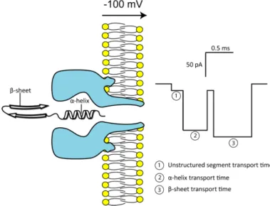
In parallel with the nanopore analysis of DNA, several groups have reported that peptide and protein molecules could be analyzed in the same way. Based on the idea proposed by Singer that polypeptides translocate through chan-nels in vivo [28]. Initial studies on peptides showed that different sequences have different values of Iblock and Tblock. For instance, while for the ↵-helical
peptides, both Iblock and Tblock increase with the length, on the other hand
for the -sheet structures smaller values of Iblock and Tblock are reported
com-pared with ↵-helix (Fig. 1.10). This breakthrough indicated that nanopore sensing could be used to conduct structural and conformational studies of peptides and proteins, enabling the collection of results difficult to obtain by bulk spectroscopic techniques such as circular dichroism (CD) or nuclear magnetic resonance (NMR). Thus, although it is not possible to identify with certainty a particular structure based on the values of Iblock and Tblock,
tentative assignments can be made comparing them with previous data [29].
Figure 1.10: Schematic representation of the ↵-hemolysin pore inserted into a lipid bilayer with ↵-helical and -sheet segments of a protein ready for translocation. The transit of differently folded segments should be reflected within the translocation profile of each protein molecule.
Furthermore, the peptides had much lower charge densities than DNA which was reflected in transit times of 1 to 2 orders of magnitude longer, re-sulting in increased signal resolution compared to nucleic acids. It was found that the number of events per time increased with the applied electric poten-tial and decreased with the peptide length [30]. However, sequencing peptides
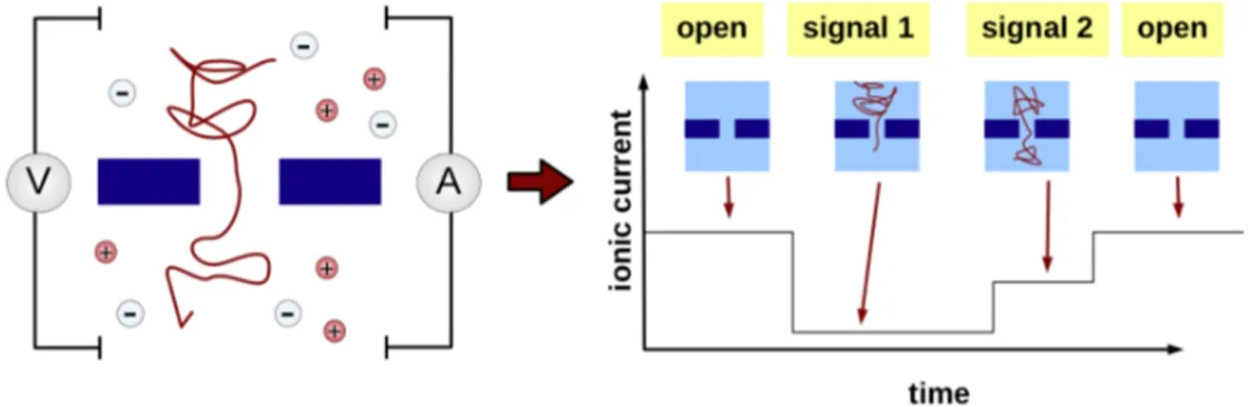
Nanopore for Bio-Molecules State of the Art and proteins by nanopores are even more challenging because there are 20 common amino acids and some of which are chemically very similar, there is also the problem that neutral peptides cannot be driven through the pore. The richness of information obtained from the nanopore analysis of peptides proved that different secondary and tertiary structures can be individually identified and distinguished, suggesting that nanopore sensing could be used to help elucidate one of the most intriguing problems of modern biochem-istry: the folding mechanism of proteins [31]. Protein misfolding is believed to be the primary cause of Alzheimer’s disease (AD), Parkinson’s disease, Huntington’s disease, the "prion" diseases such as Creutzfeldt-Jakob disease, cystic fibrosis, amyotrophic lateral sclerosis and many other degenerative and neurodegenerative disorders. Regardless of the type, the post-mortem analy-sis of brain tissue shows the presence of amyloid fibrils, plaque which conanaly-sist of protein aggregates. Surprisingly, the proteins show no obvious sequence or structural homology; the fact that the proteins are not in their native conformations has led to the hypothesis that they are all "protein misfolding diseases" [32]. Misfolded proteins are normally sequestered or neutralized by cellular defense mechanisms which include the chaperone, proteasome and/or auto-phagosome responses, one possibility is that these responses are affected during AD as well as the normal protein turnover, which is essential for cell survival, not for functional aspects. Whatever is the real mechanism of ac-tion, the presence, and the subsequent misfolded peptides play a central role in this pathological condition [33]. It is perhaps surprising that there is no definitive structure for any of the misfolded proteins. The problem is that at high concentrations they inevitably aggregate which precludes the use of NMR or X-ray crystallography. Nanopore analysis is ideally suited for study-ing peptides which can adopt multiple conformations since each molecule is interrogated individually (Fig. 1.11). It is also very sensitive since in the-ory a single molecule can be detected. Therefore, the experiments can be performed at relatively low concentrations so that aggregates will only form slowly if at all.
The issue in protein’s measurement is the transport of the analysis to and through the pore, with electrophoresis, which is very useful in nanopore DNA measurement, is less effective for neutral or weakly charged species. A technique using unmodified nanopores that facilitates protein translocation and enables specific protein identification [34]. The use of double-stranded DNA carrier molecules capable of binding one or more analytes. The highly charged DNA can electrophoretically transport the bound protein through the nanopore for sensing, and the binding site selectivity enables highly spe-cific detection. This approach was also able to identify a single analyte from a mixture. The Synthesis of DNA strands capable of binding to specific
Nanopore for Bio-Molecules State of the Art
Figure 1.11: Schematic of the translocation of a protein through a nanopore. Denaturing agents impart a uniform negative charge to the protein, resulting in a rod-like structure
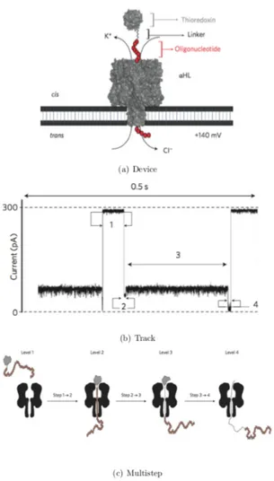
biomolecules is able to give a binary indication of their presence in a solution containing the target and a background mixture. With further improvement in data analysis or binding site design, quantitative concentration determi-nation may also be possible. This technique is highly generalizable a DNA carrier can be easily designed and created for any combination of specific ligand-receptor binding pairs. The adaptability of this platform opens many possibilities including detection of antibodies and single molecules inacces-sible with other techniques. It is demonstrated the ability of nanopores, to distinguish between folded and unfolded states of proteins at the single-molecule level. These experiments reveal additional detail, such as the exis-tence of intermediates. In total, it observes different steps in the translocation process (Fig. 1.12). The pull causes partial unfolding, the unfolding rate has an exponential dependence on the applied potential. The partial unfolding destabilizes the remainder of the folded structure, which then unfolds spon-taneously and diffuses through the pore. The experiments showed also how the passage through the pore depending on the applied potential and the exit of the pore independent of voltage [35].
Nanopore for Bio-Molecules State of the Art
Figure 1.12: (a) The pore is inserted into a lipid bilayer from the cis compartment and a potential is applied, causing an ionic current to flow through the pore. (b) Current trace translocation. (c) Level 1: Peptide (V5-C109-oligo(dC)30) is in so-lution and the pore is unoccupied. Level 2: the oligonucleotide threads into the pore and pulls on the protein. Level 3: the pulling force causes partial unfolding, allowing the oligonucleotide to traverse the pore and the unfolded segment of the polypeptide to enter. Level 4: the remainder of the polypeptide unfolds spontaneously, diffuses through the pore and leaves through the trans entrance.
In conclusion, many neurodegenerative diseases involve protein misfolding into insoluble fibrils or amyloid plaques. The misfolding processes, partic-ularly the first steps, are very difficult to study by conventional techniques because at high concentrations the proteins inevitably aggregate. Nanopore analysis, being a single molecule technique, is an attractive alternative be-cause it can be performed at very low concentrations.
Atomistic Approaches to Nanopore State of the Art
1.3 Atomistic Approaches to Nanopore
Computer simulations of molecular models can give insight into microscopic processes such as nanopore translocation to further our understanding of experimental observations, potentially providing the basis for new or re-fined experimental approaches. Recent advances in genetic sequencing using nanopores implicate a fast and cheap method of sequencing, given suitable refinement. A greater understanding of the microscopic translocation factors could greatly aid in this regard, which may be achieved through simulation. Given modern resources one cannot arbitrarily replicate nature in simulations to a subatomic level of precision, however, there are techniques for replicating nature in probabilistic detail, atomic detail, even sub-atomic quantum detail [36].
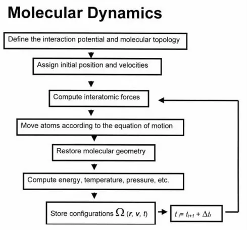
Molecular Dynamics (MD) simulations calculate the Newtonian equa-tions of motion of all particles in the system based on the forces present and recalculate the positions of the particles for a small increment in time, usually 1 or 2 femtoseconds. The deterministic time-evolution of the sys-tem is calculated in this way, the accuracy of which depends on the level of detail in the model and interactions supplied and allowed. Due to current limits in the timestep of each recalculation, there are limits on the timescales that can be simulated in atomistically detailed MD. Such limits are typi-cally in terms of nanoseconds, but with the increasing availability and scope of high-performance computing facilities, there are instances of microsecond timescales [37] and even millisecond timescales [38]. Since MD simulations reproduce the deterministic time-evolution, they allow for the calculation of the dynamics of the system.
Simulations can also be performed at the quantum sub-atomic level. In MD simulations, the model of interactions between the atoms of the system is supplied as the simulation’s input, which requires prior knowledge about the interactions of the system. Ab-initio, on the other hand, uses the laws of quantum mechanics to calculate atomic interactions. The main value in Ab-initio is that bond breaking and bond forming is accounted for, unlike in classical MD.
Chapter 2
Theoretical Methods
In this chapter methods for the computer simulations are detailed. Using these methods it is possible to gain insight into such systems and produce important features of a process. Through a greater level of understanding unlocked by simulations, we can understand more about biological processes, and it is possible to design improved experimental components and conditions.
2.1 Molecular Dynamics
In this approach all atoms in the system are treated as classical particles moving under the influence of the Newton’s classical equations of motion [39].
mi
d2
dt2R~1(t) = ~Fi(t) = rV ( ~Ri(t), ..., ~Rn(t)) (2.1)
Where ~Ri and mi denote the position and the mass of the atom i
respec-tively, and n the total number of atoms in the system. The force ~Fi acts
on atom i and is determined as the gradient of the potential energy V ( ~R(t)) of the system. The empirical force fields describe the potential energy of the system in terms of the interactions between the atoms. In its functional form, the potential energy function has two kinds of parameters, bonded and non-bonded ones. The former class consists of potentials for bond lengths, bond angles, improper dihedral angles as well as torsional angles. The later class contains the non-bonding terms, the electrostatic as well as the Van der Waals interactions. The parameters for the force fields are obtained with quantum-mechanical calculations which can be further improved by fitting to experimental data. Among the force fields commonly used in MD simula-tion of biomolecules there are CHARMM [40], AMBER and GROMOS. The
Molecular Dynamics Theoretical Methods various force fields may differ in the functional form of individual terms and especially in the parametrization procedures for the large number of param-eters involved. One of the biggest advantages of the MD technique is the brief time required to obtain the atomic details and the structural analysis of the molecular system. Unfortunately this advantage comes at a large com-putational cost. Moreover, one has to keep in mind that various biological processes occur at time scales ranging from femtoseconds over milliseconds to seconds (ex. protein folding being on the slower side of this spectrum). This has to be seen in connection to the usual MD time step in the femtosec-onds range for state-vibrational (such as hydrogen bond vibrations). With the present computational resources, simulations in the range of a few hun-dreds of nanoseconds are the common practice which may be extended up to several microseconds [41].
Although MD simulations have been very successful providing micro-scopic details of biological processes, several limitations associated with the method have to be taken into account. Standard force fields used in bio-molecular simulations account for electrostatic interactions and the corre-sponding interactions are often based on a simple pairwise-additive models, and real physical systems undergo substantial polarization when placed into a medium with a high dielectric constant such as water or in the presence of an external applied electric field. Polarizable force fields are available to explicitly account for many-body induced polarization effects but they are computationally more expensive [42].
2.1.1 Steered Molecular Dynamics
Steered Molecular Dynamics (SMD) provides a means of retrieving more data in a smaller timescale while keeping atomistic detail. This comes at the cost of the system being at non-equilibrium. Approximations do not necessarily have to take the form of model simplifications, MD programs such as NAMD [43] allow simulated processes to be steered by introducing non-equilibrium forces. The SMD allows to apply a directional force an atom, causing the atoms and anything coupled to the atoms to move along the direction of the force. The benefit of this is that a significant degree of movement can be induced in a relatively short timeframe, and the full atomistic dynamics of the process can be examined. Applying SMD to threading molecule’s chains through nanopores, the translocation process can be replicated in a atomistic model within a timeframe that can be simulated. By pulling the molecule strand at constant velocity (known as constant velocity steered MD or cv-SMD [43]), a translocation of known distance can be performed. In constant velocity SMD, an atom or the centre of a group of atoms is harmonically
Molecular Dynamics Theoretical Methods restrained to a point in space that is shifted in the chosen direction. The harmonic restraint can be thought of as a spring attached to a dummy atom, the strength of the restraint is given by a force constant k (figure 2.1). The simulation outputs the force in pico-newtons (pN) experienced by the spring in the direction of pulling (the reaction coordinate). This dummy atom is moved at constant velocity and then the force between both is measured using: ~ F = rU (2.2) U = 1 2k[vt (~r ~r0)· ~n] 2 (2.3)
Where U is potential energy, k is spring constant, v is pulling velocity, t is time, ~r and ~r0 are actual position and initial position of the SMD atom, ~n
is direction of pulling.
Figure 2.1: Pulling in a one-dimensional case. The dummy atom is colored red, and the SMD atom blue. As the dummy atom moves at constant velocity the SMD atom experiences a force that depends linearly on the distance between both atoms.
An alternative to cv-SMD is constant force SMD (cf-SMD), here the con-straint point is moved to keep the force on the recon-straint at a constant value, resulting in a variable velocity. This is advantageous when the applied force must remain limited, but one loses control over translocation time, hence the length of the simulation. Therefore cf-SMD is not applicable for these simulations.
Molecular Dynamics Theoretical Methods Ionic Current
Ionic current measurements are used to characterize single nanopores and their interactions with biological molecules; the current is calculated with the equation 2.4 I(t + t/2) = 1 tlz N X i=1 qi(zi(t + t) zi(t)) (2.4)
Where zi and qi are respectively the z-coordinate and charge of ion i, t
is the simulation time and lz is the lenght of the cell along z.
Density Functional Theory Theoretical Methods
2.2 Density Functional Theory
Density Functional Theory (DFT) is a method which determines the ground state of a system of N electrons. The DFT is one of the most popular ab initio methods which is interested in the total electronic density at each point in space, rather than attempting to obtain the many-particle wavefunction directly. DFT has proved to be succesful in accounting for structural and electronic properties of a vast class of materials, ranging from atoms and molecules to crystals and other complex extended systems.
The fundamental Schr¨odinger equation governing the full quantum me-chanics of atoms and electrons has been well known since the 1920’s [44]. However, the task of solving these equations for realistic systems is tremen-dous. For electrons and nuclei interacting through the Coulomb force the Hamiltonian is: ˆ H = ˆTe+ ˆVe e+ ˆVe n+ ˆTn+ ˆVn n = X i ~2 2mer 2 i + X i6=j e2 2|~ri ~rj| X i,A ZAe2 |~ri R~A| X i ~2 2MAr 2 A+ X A6=B ZAZBe2 2| ~RA R~B| (2.5) The first two terms represent the electronic kinetic and Coulomb elec-trostatic potential energy, the third is the electron-ion attractive potential energy while the last two terms are the ion kinetic and repulsive potential energy respectively; ~ri, me and e the position, mass and charge of the
i’th electron, and A labels the corresponding nucleus parameters. Within the Born-Oppenheimer approximation [45] one decouples the electrons and nuclei by neglecting the nuclei kinetic energy. Due to the large mass dif-ference (mA/mi ⇡ 1823ZA) the nuclei move on a much longer time scale
and the electronic structure only depends parametrically on the nuclear co-ordinates. Hence one thinks of the Coulomb repulsion between electrons and nuclei together with external fields as an external potential. The solid success of DFT lies in the possibility of a complete description of a many-body ground state from the density of an noninteracting system with an effective potential. This is the essence of the Hohenberg-Kohn theorems [46] applied in the KS-theory due to Kohn and Sham [47]. According to the theorem by Hohenberg and Kohn a system’s external potential and the cor-responding ground state energy is a unique functional of the ground state density. Therefore, the full Hamiltonian and all properties can be regarded
Density Functional Theory Theoretical Methods as a functional of the ground state density. In the Kohn-Sham procedure one replaces the Hamiltonian of the interacting many-body problem with that of a noninteracting auxiliary system with an effective potential reproducing the correct ground state energy. In this way one reduce the problem to having to solve a sequence of single-particle equations self-consistently with a generally unknown exchange-correlation potential describing all quantum many-body interactions. A variety of different exchange-correlation functionals exist. In this project only the most common Local Density Approximation (LDA) or Generalized Gradient Approximation (GGA-PBE) are used for exchange and correlations [48].
The Hohenberg-Kohn Theorems
At the base of the DFT as it is known today, there are Hohenberg-Kohn Theorems published in 1964 [46]. The first Hohenberg-Kohn theorem states that the electron density is uniquely determined by the Hamiltonian opera-tor and thus so are all the properties of the system. This implies that the external potential Vext(~r) is (to within a constant) a unique functional of
electronic density ⇢(~r). As the external potential Vext(~r) specifies the whole
Hamiltonian, the full many particle ground state is a unique functional of the electron density ⇢(~r). Thus, ⇢(~r) determines the number of electrons N and the external potential Vext(~r) and consequently all the properties of the
ground state. The total energy functional E[⇢] can be written as, E[⇢] =
Z
⇢(~r)Vext(~r)d~r + FHK[⇢] (2.6)
FHK[⇢] = T [⇢] + Eee[⇢] (2.7)
The first term in Equation 2.6 represents the potential energy due to the electron-nuclei interaction, and FHK[⇢] is an unknown, but otherwise
universal functional of the electron density ⇢(~r) only. If it was known, the solubility of Schr¨odinger equation would be possible for any system. The FHK[⇢] functional consists of a kinetic energy functional T [⇢] and
electron-electron repulsive interaction functional Eee[⇢]. The second Hohenberg-Kohn
theorem is nothing more than the variational principle. It states that the electronic density that minimizes the total energy is the exact ground state density. That is for a trial density ˜⇢(~r) we have
E0 E[˜⇢(~r)] = T [˜⇢] +
Z ˜
Density Functional Theory Theoretical Methods which means that the energy resulting from Equation 2.6, using the trial density ˜⇢(~r), represents an upper bound to the true ground state energy E0.
E0 is the outcome if and only if the exact ground state density is used in
Equation 2.8.
The Kohn-Sham Theory
The ground state energy of a system is by given the minimum of the Equation 2.8.The functional FHK[⇢] can be defined as
FHK[⇢] = T [⇢] + Eee[⇢] = T [⇢] + J[⇢] + Enc[⇢] (2.9)
where T [⇢], J[⇢], and Enc[⇢]are respectively the kinetic energy, the
classi-cal Coulomb interaction and the non-classiclassi-cal functional; of these functionals, only J[⇢] is known. The Kohn-Sham theorem provides an effective way to express T [⇢] and Enc[⇢] [47]. The idea of the Kohn-Sham approach is to
use the kinetic energy of a fictitious non-interacting system Tswith the same
electronic density as the real interacting one instead of the true kinetic energy T [⇢], where Ts = ~ 2 2m N X i h i|r2| ii (2.10) ⇢s(~r) = N X i X & | i(~r, &)|2 = ⇢(~r) (2.11) i(~r, &) are then the spin-orbital wave functions of the fictitious
non-interacting system. The two kinetic energies of the real and fictitious system are different, however, this difference is taken into account by introducing a new functional called exchange-correlation energy which contains everything that is unknown for us. Hence the functional FHK[⇢]takes the following new
form
FHK[⇢] = Ts[⇢] + J[⇢] + Exc[⇢] (2.12)
Exc[⇢] = T [⇢] Ts[⇢] + (Eee[⇢] J[⇢]) = T [⇢] Ts[⇢] + Enc[⇢] (2.13)
Calculating the Ts[⇢]requires knowing the orbitals iof the non-interacting
system. If the potential is characterized by the same density as the real sys-tem, it can be re-written Equation 2.6 using Equation 2.12
Density Functional Theory Theoretical Methods E[⇢] =
Z
⇢(~r)Vext(~r)d~r + Ts[⇢] + J[⇢] + Exc[⇢] (2.14)
Using Equations 2.9 through 2.12 in 2.14 gives the set of Kohn-Sham equations: ( ~ 2 2mr 2+ V ef f(~r1)) i = ✏i i (2.15) Vef f(~r1) = Z ⇢(~r2) |~r1 ~r2| d~r2+ Vx(~r1) M X A ZAe2 |~r1 ~rA| (2.16)
The second term in effective potential Vef f represents the exchange-correlation
potential and defined as the derivative of energy functional with respect to electronic density
Vxc =
@Exc
@⇢ (2.17)
Knowing the three terms in Equation 2.16, determines the potential Vef f which consequently determines the energy and electronic density of the
ground state. As the potential Vef f depends on density, the Kohn-Sham
equations have to be solved iteratively. It is worth pointing out that if the exact forms of Excand Vxcwere known, the Kohn-Sham approach would lead
to the exact ground state energy. These functionals have unknown forms and using the Kohn-Sham in practice requires finding reasonable approximations. The Exchange-Correlation Functionals
The local density approximation LDA
The first expression for the exchange-correlation functional Exc was
orig-inally derived to describe the exchange effects in a homogeneous electron gas (HEG). In HEG, the electrons move in the presence of a background of positive charge which ensures the overall charge neutrality of the system. As the exchange energy of a HEG depends upon the local value of electronic density, the term "local density approximation (LDA)" is used to refer to those functionals based on HEG. The LDA is the basis of all approximate exchange-correlation functionals. According to LDA, the energy functional Exc can be expressed in the form
ExcLDA[⇢] =
Z
Density Functional Theory Theoretical Methods where ✏xc([⇢], ~r) is the exchange-correlation energy per electron, at
posi-tion (~r), of a uniform electron gas of density ⇢(~r). For the unpolarized system, this energy depends only on the value of electronic density in some neigh-borhood of position (~r). In the LDA approximation the exchange potential is equal to VxcLDA(~r1) = e2 ⇡[3⇡ 2⇢(~r 2)]1/3 (2.19)
The generalized gradient approximation GGA
In order to improve the LDA, the so-called Generalized Gradient Ap-proximation (GGA), where the gradient of the density is also considered, has been introduced [49]. In comparison with LDA, GGA tends to improve total energies, atomization energies, energy barriers and structural energy differences. In GGA, the exchange-correlation energy depends both on the homogeneous electron gas density and on its gradient:
Excxc[⇢] = Z
f (⇢(~r),r⇢(~r)d~r (2.20) where f is a parametrized analytic function. To obtain reasonable results the function f must be chosen with care, because the expression 2.20 does not derive from a physical system. The xc-functional used for most of the calculations presented in this thesis is the Perdew-Burke-Ernzerhof (PBE) functional [48].
Pseudopotentials
The pseudopotentials replace the strong Coulomb potential of the nucleus and the effects of the tightly bound core electrons with an ionic potential acting on the valence electrons. The valence electrons are the principal re-sponsible for chemical bonds in materials. In some cases the wavefunctions representing valence electrons of some external shell (3d or 4f for instance), strongly oscillates, and so for sampling these wavefunction a huge number of plane waves is needed, wasting the computational efficiency of the simu-lation. Thus, the main reasons for the introduction of pseudo-potentials are reduction of basis set size, reduction of number of electrons and inclusion of relativistic or other effects. Electron-ion core interactions are typically represented by a non-local norm-conserving pseudopotential (NCPP), a soft potential for valence electrons only, so that core electrons disappear from the calculation; for a given reference configuration they must meet some reason-able conditions:
Density Functional Theory Theoretical Methods • the electron energy level must be the same in full all-electron
calcula-tions and calculacalcula-tions made with pseudopotentials ✏ps = ✏ae
• the new wavefuction obtained via pseudopotentials must be nodeless. • the two wavefunctions must coincide from a certain value of the radial
variables in order the reproduce the scattering properties of the true potential ps
l (r) = ael (r) or r > rc.
• the charge inside rc for each wavefunctions agrees (norm-conservation):
Z r<rc r2dr| psl (r)|2 = Z r<rc r2dr| psl (r)|2 (2.21) where l(r) is the radial part of the atomic valence wavefunction with
angular momentum specified by the quantum number l and the core radius rc is approximately at the outermost maximum of the wavefunction.
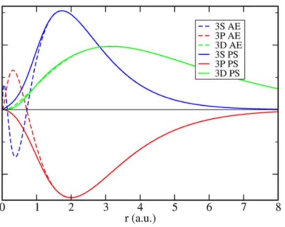
Figure 2.3: All electron calculations vs. Pseudopotential for the radial part of wavefunctions 3s, 3p and 3d.
Quantum Transport Theory Theoretical Methods
2.3 Quantum Transport Theory
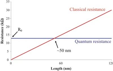
According to Ohm’s law, the resistance R of a conductor is directly propor-tional to its length L and inversely proporpropor-tional to its cross-secpropor-tional area A; that is, R = V/I = (⇢L)/A, where ⇢ is the resistivity and it is characteristic of the conductor material. The reciprocal of the resistance is the conduc-tance G, G = 1/R = A/L, where = 1/⇢ is the conductivity. Equation of G suggests that the conductance of a conductor increases indefinitely by de-creasing its length. However, the experimental results showed that this ohmic behaviour breaks down at some critical value of the conductor length. Below this specific length, the conductance reaches its maximum value and decreas-ing the length has no effect on G. In other words, as illustrated schematically in Figure 2.4, the resistance of any conductor cannot be reduced to less than a minimum finite value R0.
Figure 2.4: The resistance of a conductor vs its length. Adapted from "www.quantumwise.com"
Thus, concepts like Ohm’s law are not applicable at the atomic scale. As the length of the conductor is reduced to the atomic scale such that the conductor is just an individual molecule, the effect of quantum phenomena becomes more important and dominates the conducting process; the finite resistance is associated with the resistance arising at the interfaces between leads and the sample in between them [50]. This can lead to an unexpected and incongruous behaviour to the classical one, such as a resistance that is independent of molecule length, non-linear I V characteristics and even negative differential resistance. Atomic-size conductors are a limiting case of systems in which quantum coherence plays a central role in the transport properties. A conductor would exhibit various transport regimes
depend-Quantum Transport Theory Theoretical Methods ing upon its dimensions relative to three characteristic length scales [51]; a fundamental length scale is the phase coherence length, L which mea-sures the distance over which the phase of the electron wave function is pre-served (phase coherence can be destroyed by inelastic scattering mechanisms like electron-electron or electron-phonon interactions), the mean free path l which measures the distance between static collision with static scatterers and the de Broglie wavelength [52]. These regimes can be summarized as the following:
• Mesoscopic if ⌧ L < L • Diffusive if L and L l • Ballistic if L > l
• Quantum transport if ⇠ L
The diffusive and ballistic transport can be described using classical or semi-classical laws, in a semiclassical model the electron motion is a random walk of steps l among the impurities; when we reach the ballistic regime the electron momentum can be assumed to be constant and only limited by the scattering with the geometric boundaries of the sample. Whereas quantum transport phenomena (where the typical dimensions of the sample are within atomic-scale) are fully governed by quantum mechanics. The mesoscopic regime would be a separate kingdom governed by separate laws that are neither purely quantum nor purely classical; rather, a synthesis of the two. If the dimensions of the conductor are much larger than each of the three length scales, the conductor shows ohmic behaviour.
2.3.1 Elastic Transport
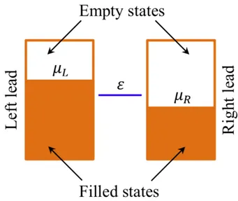
To study the quantum transport through an individual molecule, we will introduce a simple model for electronic transport [53]; Figure 2.5 shows the energy level diagram of a molecule with a single energy level sandwiched between metal leads.
Both leads are assumed to contain a continuum of states, which extends to all energies, and which is filled up to some Fermi level µL and µR; the
molecule is coupled to both leads with coupling constants L and R which
have units of energy. Physically, L and R(divided by ~) represent the rate
at which an electron in the molecule’s energy level ✏ would escape into left lead and right lead, respectively. The stronger coupling the higher probability
Quantum Transport Theory Theoretical Methods
Figure 2.5: A molecule with one energy level in between two leads.
for escaping. If the energy level of the molecule was in equilibrium with the left lead, then the number of electrons occupying the level would be given by NL = 2f (✏, µL) (2.22)
f (✏, µ) = 1 1 + expk✏ µ
BT
(2.23) where the factor 2 is for spin degeneracy and f is the Fermi distribution function. Similarly, if the level was in equilibrium with the right lead, the number of electrons occupying the level would be, NR = 2f (✏, µR). Under
non-equilibrium conditions, the number of electrons N will be somewhere in between NL and NR. To determine this number, the current is written IL at
the left junction and IR at the right junction:
IL= e L ~ (NL N ) (2.24) IR= e R ~ (N NR) (2.25)
So that from equations of IL, IR is obtained the current:
I = 2e ~
L R
L+ R
[f (✏, µL) f (✏, µR)] (2.26)
Quantum Transport Theory Theoretical Methods • No current will flow if f(✏, µL) = f (✏, µR)
• A level that is at lower energy than both Fermi levels µL and µR will
have f(✏, µL) = f (✏, µR) = 1 and will not contribute to the current.
• A level that is at higher energy than the µLand µR and has f(✏, µL) =
f (✏, µR) = 0 will not contribute also to the current.
• It is only when the molecule’s level lies between µLand µR(or within a
few kBT of µL and µR) that we have f(✏, µL)6= f(✏, µR), and a current
flows.
The maximum current that can flow through one molecular level is equal to, Imax = 2e~ LL R+ R. The figure 2.6 shows a typical I V characteristics of one
energy level calculated from equation 2.26 for different parameters. It can be seen that, at small bias voltages, the current is zero because both µL and µR
are above the molecule energy level. When the voltage becomes sufficiently high, the µR drops below the energy level and the current increases to the
maximum value Imax. It is worth noting that, the size of the gap in the
current-voltage curve is equal to 4|Ef ✏0|. Ef is the Fermi level of the
system (left lead + molecule + right lead) at equilibrium, i.e. V = 0.
Figure 2.6: (Right) The current-voltage (I-V) characteristics of a single energy level with µL= Ef eV /2, µR= Ev+eV /2. (Left)The Voltage dependence position
of the energy level relative to the µL and µR.
When the current flows through the molecule of single energy level, elec-trons are added to or removed from the level continuously leading to what is called "charging effects". These effects have not been taken into account. The change in electron occupation of the energy level modifies the potential in the molecule. In order to make the model more realistic, we should include effects of charging.
Quantum Transport Theory Theoretical Methods Non-Equilibrium Green’s Function and
Landauer-Büttiker Formula
The simple model introduced in the previous section shed some light on basic factors that influence molecular conduction, but it does not describe two important aspects of a real device: the electronic structure of the contacts and the details of the scattering region Hamiltonian. These are replaced respectively by the Fermi distribution functions and by a single energy level. In reality, the molecular devices typically have multiple energy levels that broaden and overlap with each other and with the contacts levels. The non-equilibrium Green’s function (NEGF) formalism does just that. The figure 2.7 shows a typical molecule in between two metal leads.
Figure 2.7: molecule sandwiched between two leads.
To investigate the electrical conduction through the molecule, the system is divided into three regions: the left lead, the right lead, and the scattering (central) region where the molecule of interest is located. The part of the scattering region where the atom positions follow the periodic arrangement of the leads is called the left and right lead extension. A sufficient fraction of the leads are included in the scattering region to screen out the perturbation of the scatterer, i.e. the molecule, in the outermost part of the scattering region. Since the two leads are semi-infinitely extended to the left and right sides (where the periodic boundary conditions are applied), the Hamiltonian of the whole system will be infinite in size. However, it can be computed by exploiting the periodic nature of the leads from smaller calculable compo-nents. To calculate the Hamiltonian of the system, for each lead a principal unit cell of calculation is chosen, which is at minimum the smallest number of atomic layers required so that no coupling exists between next nearest unit cells. As illustrated in Figure 2.8, each principal unit cell now has a finite Hamiltonian HL and HR, and another matrix which describes the
Quantum Transport Theory Theoretical Methods HRC. The scattering region also has a finite Hamiltonian HS and coupling
matrices between itself and each lead HSLC and HSRC.
Figure 2.8: Schematic diagram shows how the Hamiltonian of the one dimensional system is built up. In this example, each red rectangle, with two atoms, represents one principal unit cell of the lead, and the blue rectangle represents the scattering region which consists of left and right lead extensions and the molecule of interest.
The Hamiltonian H describing the system can then be written as: H = 2 4HH+L HSLC 0 SLC HS H+SRC 0 HSRC HR 3 5 (2.27) The overlap matrix S can be obtained in the same manner; for a single energy level ✏, the Green’s function is defined as:
G(E) = (E ✏ + i L+ R 2 )
1 (2.28)
and in the case of the whole (infinite) system, the Green’s function equa-tion is given by
[(E + i⌧ )S H]G(E) = I (2.29) where ⌧ is infinitesimal small positive number added to avoid singularity in calculation. I is the identity matrix with the same size of S and H. What is required to calculate the current is the central block of the Green’s function that corresponds to the scattering region (i.e. the molecule + leads
![Figure 1: Illustration of a single-stranded DNA molecule passing through ↵HL nanopore [2].](https://thumb-eu.123doks.com/thumbv2/123dokorg/2893245.11390/8.892.217.680.773.996/figure-illustration-single-stranded-dna-molecule-passing-nanopore.webp)
![Figure 1.4: Solid-statenanopores fabricated with two-dimensional nanomem- nanomem-branes: a a graphene nanopore; b a BN nanopore; c a MoS2 nanopore; [15–17].](https://thumb-eu.123doks.com/thumbv2/123dokorg/2893245.11390/14.892.184.707.474.829/figure-statenanopores-fabricated-dimensional-graphene-nanopore-nanopore-nanopore.webp)