DOI:10.1051/0004-6361/201628890 c ESO 2016
Astronomy
&
Astrophysics
Planck intermediate results
XLVI. Reduction of large-scale systematic effects in HFI polarization maps
and estimation of the reionization optical depth
Planck Collaboration: N. Aghanim53, M. Ashdown63, 6, J. Aumont53, C. Baccigalupi75, M. Ballardini29, 45, 48, A. J. Banday85, 9, R. B. Barreiro58,
N. Bartolo28, 59, S. Basak75, R. Battye61, K. Benabed54, 84, J.-P. Bernard85, 9, M. Bersanelli32, 46, P. Bielewicz72, 9, 75, J. J. Bock60, 10, A. Bonaldi61,
L. Bonavera16, J. R. Bond8, J. Borrill12, 81, F. R. Bouchet54, 79, F. Boulanger53, M. Bucher1, C. Burigana45, 30, 48, R. C. Butler45, E. Calabrese82,
J.-F. Cardoso66, 1, 54, J. Carron21, A. Challinor55, 63, 11, H. C. Chiang23, 7, L. P. L. Colombo19, 60, C. Combet67, B. Comis67, A. Coulais65,
B. P. Crill60, 10, A. Curto58, 6, 63, F. Cuttaia45, R. J. Davis61, P. de Bernardis31, A. de Rosa45, G. de Zotti42, 75, J. Delabrouille1, J.-M. Delouis54, 84,
E. Di Valentino54, 79, C. Dickinson61, J. M. Diego58, O. Doré60, 10, M. Douspis53, A. Ducout54, 52, X. Dupac36, G. Efstathiou55, F. Elsner20, 54, 84,
T. A. Enßlin70, H. K. Eriksen56, E. Falgarone65, Y. Fantaye34, F. Finelli45, 48, F. Forastieri30, 49, M. Frailis44, A. A. Fraisse23, E. Franceschi45,
A. Frolov78, S. Galeotta44, S. Galli62, K. Ganga1, R. T. Génova-Santos57, 15, M. Gerbino83, 74, 31, T. Ghosh53, J. González-Nuevo16, 58,
K. M. Górski60, 87, S. Gratton63, 55, A. Gruppuso45, 48, J. E. Gudmundsson83, 74, 23, F. K. Hansen56, G. Helou10, S. Henrot-Versillé64, D. Herranz58,
E. Hivon54, 84, Z. Huang8, S. Ili´c85, 9, 5, A. H. Jaffe52, W. C. Jones23, E. Keihänen22, R. Keskitalo12, T. S. Kisner69, L. Knox25, N. Krachmalnicoff32,
M. Kunz14, 53, 2, H. Kurki-Suonio22, 41, G. Lagache4, 53, J.-M. Lamarre65, M. Langer53, A. Lasenby6, 63, M. Lattanzi30, 49, C. R. Lawrence60,
M. Le Jeune1, J. P. Leahy61, F. Levrier65, M. Liguori28, 59, P. B. Lilje56, M. López-Caniego36, Y.-Z. Ma61, 76, J. F. Macías-Pérez67, G. Maggio44,
A. Mangilli53, 64, M. Maris44, P. G. Martin8, E. Martínez-González58, S. Matarrese28, 59, 38, N. Mauri48, J. D. McEwen71, P. R. Meinhold26,
A. Melchiorri31, 50, A. Mennella32, 46, M. Migliaccio55, 63, M.-A. Miville-Deschênes53, 8, D. Molinari30, 45, 49, A. Moneti54, L. Montier85, 9,
G. Morgante45, A. Moss77, S. Mottet54, 79, P. Naselsky73, 35, P. Natoli30, 3, 49, C. A. Oxborrow13, L. Pagano31, 50, D. Paoletti45, 48, B. Partridge40,
G. Patanchon1, L. Patrizii48, O. Perdereau64, L. Perotto67, V. Pettorino39, F. Piacentini31, S. Plaszczynski64, L. Polastri30, 49, G. Polenta3, 43,
J.-L. Puget53,?, J. P. Rachen17, 70, B. Racine1, M. Reinecke70, M. Remazeilles61, 53, 1, A. Renzi34, 51, G. Rocha60, 10, M. Rossetti32, 46,
G. Roudier1, 65, 60, J. A. Rubiño-Martín57, 15, B. Ruiz-Granados86, L. Salvati31, M. Sandri45, M. Savelainen22, 41, D. Scott18, G. Sirri48,
R. Sunyaev70, 80, A.-S. Suur-Uski22, 41, J. A. Tauber37, M. Tenti47, L. Toffolatti16, 58, 45, M. Tomasi32, 46, M. Tristram64, T. Trombetti45, 30,
J. Valiviita22, 41, F. Van Tent68, L. Vibert53, P. Vielva58, F. Villa45, N. Vittorio33, B. D. Wandelt54, 84, 27, R. Watson61,
I. K. Wehus60, 56, M. White24, A. Zacchei44, and A. Zonca26
(Affiliations can be found after the references) Received 10 May 2016/ Accepted 14 July 2016
ABSTRACT
This paper describes the identification, modelling, and removal of previously unexplained systematic effects in the polarization data of the Planck High Frequency Instrument (HFI) on large angular scales, including new mapmaking and calibration procedures, new and more complete end-to-end simulations, and a set of robust internal consistency checks on the resulting maps. These maps, at 100, 143, 217, and 353 GHz, are early versions of those that will be released in final form later in 2016. The improvements allow us to determine the cosmic reionization optical depth τ using, for the first time, the low-multipole EE data from HFI, reducing significantly the central value and uncertainty, and hence the upper limit. Two different likelihood procedures are used to constrain τ from two estimators of the CMB E- and B-mode angular power spectra at 100 and 143 GHz, after debiasing the spectra from a small remaining systematic contamination. These all give fully consistent results. A further consistency test is performed using cross-correlations derived from the Low Frequency Instrument maps of the Planck 2015 data release and the new HFI data. For this purpose, end-to-end analyses of systematic effects from the two instruments are used to demonstrate the near independence of their dominant systematic error residuals. The tightest result comes from the HFI-based τ posterior distribution using the maximum likelihood power spectrum estimator from EE data only, giving a value 0.055 ± 0.009. In a companion paper these results are discussed in the context of the best-fit PlanckΛCDM cosmological model and recent models of reionization.
Key words. cosmology: observations – dark ages, reionization, first stars – cosmic background radiation – space vehicles: instruments – instrumentation: detectors
1. Introduction
The E-mode polarization signal of the cosmic microwave back-ground (CMB) at multipoles less than 15 is sensitive to the value of the Thomson scattering optical depth τ. In polariza-tion at large angular scales, the extra signal generated by reion-ization dominates over the signal from recombination. Cosmic microwave background polarization measurements thus provide an important constraint on models of early galaxy evolution and star formation, providing the integrated optical depth of the
? Corresponding author: J. L. Puget,
e-mail: [email protected]
entire history of reionization, which is complementary informa-tion to the lower limit on the redshift of full reionizainforma-tion provided by Lyman-α absorption in the spectra of high redshift objects (seeDijkstra 2014;Mashian et al. 2016;Robertson et al. 2015; Bouwens et al. 2015; Zitrin et al. 2015, for recent results and reviews). The reionization parameter τ is difficult to constrain with CMB temperature measurements alone as the T T power spectrum depends on the combination Ase−2τ, and τ is
degen-erate with As, the amplitude of the initial cosmological scalar
perturbations.
The B-mode polarization signal at low multipoles is created by the scattering of primordial tensor anisotropies in the CMB by
A&A 596, A107 (2016) reionized matter. This signal scales roughly as τ2. The value of
τ is thus also important for experiments constraining the tensor-to-scalar ratio, r, using the reionization peak of the B modes.
Owing to the large angular scale of the signals, τ has been measured only in full-sky measurements made from space. Hinshaw et al. (2013) report τ = 0.089 ± 0.014 from the WMAP9 analysis.Planck Collaboration XI(2016) used Planck1
polarized 353-GHz data to clean the WMAP Ka, Q, and V maps of polarized dust emission, and WMAP K-band as a template to remove polarized synchrotron emission, lowering τ from WMAP data alone by about 1σ to τ = 0.075 ± 0.013. Planck Collaboration XIII(2016) used 70-GHz polarization data at low multipoles, which were assumed to be nearly noise-limited (see Sect.4 below for new estimates of systematic ef-fects) and were cleaned using 353 GHz and 30 GHz to remove dust and synchrotron emission. This low-multipole likelihood alone gave τ = 0.067 ± 0.023. In combination with the Planck high-multipole T T likelihood, it gave τ = 0.078 ± 0.019. The combination PlanckTT+lensing gave a comparable value of τ = 0.070 ± 0.024.
The HFI 100 and 143-GHz low-multipole polarization data combined with 353-GHz to remove the Galatic dust foreground could provide tighter constraints on τ, reducing uncertainties by nearly a factor of about two with respect to the results quoted above; however, systematic errors remaining in the HFI polar-ized data at large angular scales in the 2015 Planck release led the Planck collaboration to delay their use. Since the time when the data for the 2015 release were frozen, we have made substan-tial improvements in the characterization and removal of HFI systematic errors, which we describe in this paper. The maps, simulations, and sometimes computer codes used here are re-ferred to as “pre-2016”, and are nearly identical to those in the 2016 data release to come. We note that the HFI submillimetre channels at 545 and 857 GHz are not polarization sensitive and their improvement is not discussed in this paper.
The paper is structured in the following way. Section2 anal-yses systematic errors affecting the HFI time-ordered informa-tion processing, describes tests of these errors, and describes new versions of polarized mapmaking and calibration. Section3 discusses global tests of HFI polarization at the power spec-trum level. Section4 discusses quality tests of Low Frequency Instrument (LFI) polarization data. Section5describes compo-nent separation and cross-spectra and their suitability for the measurement of τ. Section 6 describes the likelihood analysis of the τ parameter. Finally Sect.7discusses the implications of our new τ value.
These data described here are also used in an accompany-ing paper (Planck Collaboration Int. XLVII 2016) to constrain different models for the reionization history of the Universe.
2. Improvements of HFI mapmaking and calibration for low multipoles
2.1. Overview
Analysis of HFI polarization systematic effects is com-plex and technical in nature. This paper, together with
1 Planck (http://www.esa.int/Planck) is a project of the
European Space Agency (ESA), with instruments provided by two sci-entific consortia funded by ESA member states and led by Principal Investigators from France and Italy, telescope reflectors provided through a collaboration between ESA and a scientific consortium led and funded by Denmark, and additional contributions from NASA (USA).
Planck Collaboration VII(2016), completes the characterization of the HFI time-ordered information (TOI) products, extend-ing analysis of the polarization power spectra to the lowest multipoles.
The HFI TOI used in this paper are described in the 2015 data release (Planck Collaboration VII 2016), and a calibrated version is publicly available in the Planck Legacy Archive2. The spacecraft pointing solution (Planck Collaboration I 2016) and all instrumental parameters, including the focal plane geometry, cross-polar leakage parameters, and polarization angle parame-ters, are identical to those used in the 2015 release.
HFI systematic errors have been discussed extensively in earlier papers (Planck Collaboration X 2014; Planck Collaboration VII 2016) and were shown to be under control on small angular scales. Large angular scales, however, were still affected by not-fully-understood systematic effects.
The reduction of systematic errors in HFI polarization mea-surements at large angular scales reported in this paper is the result of applying a new mapmaking code, SRoll. SRoll is a polarized destriping algorithm, similar to the 2015 HFI map-making pipeline (Planck Collaboration VIII 2016), but it solves simultaneously for absolute calibration, leakage of temperature into polarization, and various other sources of systematic er-ror. Systematic residuals are removed via template fitting, us-ing HEALPix-binned rus-ings (HPR) to compress the time-ordered information. Each HPR consists of data from a given stable pointing period (ring) binned into HEALPix pixels (Górski et al. 2005). A version of this code with minor additions will be used for the final Planck data release in 2016. In its present form, SRoll reduces the systematic errors in the HFI EE polarization spectra at multipoles ` ≥ 2 to levels close to the nominal in-strumental noise. This allows a measurement of the reionization optical depth τ from the HFI alone, which was not possible at the time of the 2015 Planck data release.
The rest of this section discusses each of the specific im-provements. Section2.2introduces the end-to-end simulations used in this paper. Section 2.3 analyses the detector system noise, which sets a fundamental limit to the measurement of the polarization spectra and to τ with HFI data. (Appendix A summarizes a number of effects removed in the TOI process-ing that make a negligible contribution to the systematic error budget of polarization measurements at large angular scales.) Section2.4describes removal of the zodiacal light, and far side-lobes. Section 2.5 characterizes the systematic errors induced by non-linearities in the analogue-to-digital converters (ADCs) used in the bolometer readout electronics. These non-linearities, if uncorrected, would be the dominant source of systematic er-rors in polarization at large angular scales. Section2.6discusses all other systematic errors not corrected after the TOI processing, and mitigated by SRoll.
2.2. End-to-end simulations
End-to-end (E2E) HFI simulations, introduced for the first time in 2015 (Planck Collaboration XI 2016), include an accurate representation of the response of the instrument to sky signals, as well as known instrumental systematic errors at the TOI or ring level, all of which are propagated through the entire anal-ysis pipeline to determine their effect on the final maps. The version used in this paper runs the pre-2016 Sroll mapmaking code, described in detail in Sect.B.3. Simulations built with this pre-2016 pipeline are referred to as HFI focal plane simulations
10−3 10−2 10−1 100 101 102 Frequency [Hz] 10−1 100 101 P ow er sp ectral densit y [a rbitra ry units]
Fig. 1.Mean power spectra of the signal-subtracted, time-ordered data
from Survey 2 for each polarization-sensitive HFI frequency channel. The spectra are normalized at 0.25 Hz. Blue, green, red, and cyan rep-resent 100, 143, 217, and 353 GHz, respectively. The vertical dashed line marks the spacecraft spin frequency. The sharp spikes at high fre-quencies are the so-called 4-K cooler lines. These noise spectra are built before the time transfer function deconvolution.
(HFPSs). Three sets of HFPSs are used in this paper: HFPS1 contains 83 realizations; HFPS2 and HFPS3 contain 100 real-izations each, which can be used either separately or together.
2.3. Detector noise
Detector noise is determined through a multi-step process, start-ing with first-order correction of the TOI for ADC non-linearity, demodulation, deglitching, 4-K line removal, and time-response deconvolution. The sky signal is then estimated (using the redun-dancy of multiple scans of the same sky during each stable point-ing period) and removed, leavpoint-ing the noise, which can then be characterized (seePlanck Collaboration VII 2016, for details).
Within a frequency band, the noise power spectrum of each bolometer has a similar shape below 5 Hz. Figure1 shows the mean noise spectrum for each of the polarization-sensitive HFI channels, normalized to unity at 0.25 Hz (we are interested here in the shapes of the noise spectra, not their absolute amplitude).
Detector noise can be divided into three components (see Fig.2), with spectra varying approximately as f0 (i.e., white),
f−1, and f−2. The f0 and f−1components are uncorrelated be-tween detectors; however, the f−2 component is correlated
be-tween detectors. This component dominates below 10−2Hz, and thus below the spin frequency. Noise levels at frequencies around 0.002 Hz (much below the spin frequency) changed during the mission, reflecting variations of the Galactic cosmic ray flux with solar modulation and their effect on the temperature of the bolometer plate. These effects are corrected using a template built from the signal of the dark bolometers smoothed on minute timescales (Planck Collaboration VI 2014). The f−2component is different for spider-web bolometers (SWBs, red curves) and polarization-sensitive bolometers (PSBs, blue curves). Common glitches seen in the two silicon wafers of a PSB produce cor-related noise with a knee frequency of about 0.1 Hz (Planck Collaboration X 2014). Above 0.2 Hz, the correlated noise is at a level of 1% of the total detector noise; at twice the spin frequency
Fig. 2.Noise cross-power spectra of the 143-GHz bolometers, with the
unpolarized spider-web bolometers (SWBs) in red and the polarization-sensitive bolometers (PSBs) in blue. The low-level correlated white noise component of the PSB noise is associated with common glitches below the detection threshold. Auto-spectra are shown in black. The uncorrelated noise is in green.
(multipole `= 2 in the maps), it contributes only 10% of the total noise.
After removal of the correlated part, an uncorrelated f−1
component remains (green curve in Fig. 2) that has fknee ≈
0.2 Hz for all HFI detectors (see, e.g., Fig. 13 of Planck Collaboration X 2014). Above this frequency the noise is pre-dominantly white, with amplitude in good agreement with ground-based measurements. The 10-MΩ resistor and the capac-itor in the focal plane, read out through the same electronics as the bolometers, show only 1/ f noise below 3 mHz, showing that this additional 1/ f component is not generated in the readout. The 1/ f component of the noise is discussed in Sect.A.1, and is well approximated by a Gaussian statistical distribution, as seen in Fig.3. The low level (<10−3) non-Gaussian wings which are cut by the 3.3σ clipping of the deglitching algorithm, are not seen on 100-ring averages, which suggest that they are caused by rare events.
1/ f noise around 0.06 Hz is largely uncorrelated, and is con-stant during the mission within uncertainties. This confirms that undetected glitches do not contribute significantly, apart from a small contribution near the spin frequency. No intrinsic 1/ f noise was detected in individual bolometer ground tests, but a 1/ f component was seen in HFI focal plane unit ground calibra-tion measurements below 0.1 Hz (see, e.g., Fig. 10 ofLamarre et al. 2010), comparable to those seen in flight. Nevertheless a thermal fluctuation residual cannot be excluded.
In summary, the correlated component ( f−2) between all bolometers is mostly removed by the dark bolometer baseline removal. The weak correlated white noise (1%) between pairs of bolometers within a PSB, caused by undetected glitches, is not removed by this baseline removal procedure. The one-minute smoothing of the dark bolometer timeline used to remove this common thermal mode will leave a small correlated residual in the frequencies just above the spin frequency. Furthermore the ADC non-linearities discussed later will affect differently
A&A 596, A107 (2016)
Fig. 3.Histogram of the noise between 0.018 and 0.062 Hz (frequencies
at which it is dominated by the uncorrelated 1/ f noise) for detector 143-1a in blue, together with the best-fit Gaussian distribution in red.
each bolometer and introduce some uncorrelated residuals which might account for at least part of this 1/ f component.
In conclusion, the component of TOI noise that is uncor-related between detectors (except near the spin frequency) can be modelled with two Gaussian components, white and 1/ f . These are taken from version 8 of the FFP8 noise modelPlanck Collaboration XII(2016), adjusted to the power spectrum ob-served in the half-ring null tests. The TOI noise, and its propaga-tion to maps and power spectra, is taken in this paper as the fun-damental limitation of HFI, and the maps built with FFP8 noise give the reference for maps and power spectra in simulations.
2.4. Sky components removed in the ring making 2.4.1. Removal of zodiacal dust emission
Thermal emission from interplanetary dust – the zodiacal emis-sion – varies not only with frequency and direction, but also with time as Planck moves through the solar system. The size of the effect on temperature is small, as estimated in Planck Collaboration VIII (2016), and it was not removed from the TOI released in 2015. Rather, we reconstruct the emission us-ing the COBE Zodiacal Model (Kelsall et al. 1998) and the zo-diacal emissivity parameters found inPlanck Collaboration VIII (2016), and subtract it from the TOI of each detector prior to mapmaking.
The zodiacal emission is not expected to be intrinsically po-larized; however, HFI measures polarization by differencing the signals from quadruplets of PSBs. Since each detector has a slightly different spectral response, any component that has a different spectrum from the blackbody spectrum of the primor-dial CMB anisotropies, such as zodiacal emission, can introduce leakage of temperature into polarization. By subtracting a model of zodiacal emission from the TOI of each detector, this source of leakage is strongly suppressed.
Differences between Q and U maps made with and with-out removal of zodiacal emission show the size of the effect. At 100, 143, and 217 GHz, the zodiacal correction is less than about 100 nKCMB. At 353 GHz, it is an order of magnitude larger. If
Table 1. Estimates of the relative impact of the FSLs per bolometer within a frequency band.
Frequency Min Max Mean rms
[GHz] [%] [%] [%] [%]
100 . . . 0.074 0.101 0.086 0.010 143 . . . 0.051 0.059 0.054 0.002 217 . . . 0.048 0.053 0.051 0.002 353 . . . 0.015 0.016 0.016 <0.001 Notes. The table lists the minimum, maximum, average, and rms val-ues between the bolometers of one frequency band. These numbers are computed by convolving the FSLs with the dipole and propagating the resulting signal to the maps and power spectra to include the filtering of the destriper.
our correction was so poor that it left 25% of the emission, tem-perature leakage would contribute errors of order 25 nKCMB to
the polarization maps at 100, 143, and 217 GHz, and perhaps 100 nKCMBat 353 GHz. The effect on τ is negligible.
2.4.2. Far sidelobes
HFI far sidelobes (FSLs) are discussed in detail in Planck Collaboration VII(2016). They are dominated by radiation from the feedhorns spilling over the edge of the secondary mirror, and by radiation reflected by the secondary mirror spilling over the edge of primary mirrorr or the main baffle3. The effects of
diffraction by edges other than the mouths of the feedhorns them-selves is important only at 100 GHz, where diffraction can af-fect very low multipoles (see below). FSL variations inside a frequency band are negligible at HFI frequencies. The Planck optical system is modelled using the GRASP software4. Higher-order effects with more than one reflection and diffraction by sharp edges can be computed by GRASP, but the complexity and computational time is a strong function of the order number. We have computed the first-order FSLs for each bolometer, and then checked for a few representative bolometers that the addition of the next seven orders gives small corrections to the first-order computations.
Convolution of the sky maps with the FSL model predicts small contributions to the maps. In addition, the contributions from FSLs close to the spin axis are reduced by destriping during the mapmaking process (a contribution of FSLs on the spin-axis is completely removed by the destriper). The Galactic contribu-tions though the FSLs are similar at 100, 143, and 217 GHz since the decrease in the FSL amplitude and the increase in Galactic emission at higher frequencies roughly compensate each other. The solar dipole FSL contributions decrease with frequency, as summarized in Table1. The FSLs produce a direct dipole cali-bration shift by increasing the effective beam etendue, though the shift is reduced by the destriping. The dispersion between detec-tors is caused by the variation in the main spillover (the rays that miss the secondary mirror), which is dominated by the position of the horns in the focal plane: the bolometers further away from the symmetry axis experience a larger spillover. This effect can be used as an additional test of the fidelity of the GRASP calcula-tions used to model the FSLs.
3 Here we adopt the convention of following the light from the
detec-tors outwards, as used in the simulations.
Fig. 4.Auto-power spectra, showing the level of the simulated FSL pro-jected on the maps predicted using the GRASP model. At ` < 10, the FSL signal at all frequencies is at least two orders of magnitude smaller than the cosmological F-EE signal.
The impact of FSLs on the HFI maps depends on the scan-ning strategy, and so must be corrected in either the TOI process-ing or in buildprocess-ing the HPRs. A FSL model has been computed from the first-order GRASP calculations. Higher-order effects are absorbed, together with other residuals, into the empirical com-plex transfer functions discussed in Sect.2.6.2. The parameters of the transfer functions are then determined from the data.
Angular power spectra5from HFI pre-2016 E2E simulations
of the FSLs are displayed in Fig.4. At all HFI frequencies, the FSL effects are smaller than the fiducial F-EE power spectrum by two orders of magnitude, where we define F-xx (F-T T , F-EE, F-BB) to be the baseΛCDM power spectra from best-fit Planck 2015 cosmological parameters (Planck Collaboration XIII 2016) τ = 0.066 and upper limit r = 0.11.
The FSL signals are removed using GRASP first-order predic-tions, leaving residuals due to higher orders and uncertainties. These residuals are smaller than the effect displayed in Fig.4.
Table1provides estimates of the effects of FSLs on the rel-ative inter-calibration with respect to the average of all detectors within the same frequency band. As discussed in Sect.2.4.2, the effect of the FSLs depends on the scanning strategy, and must be removed at the HPR level. The effect on the dipole requires prop-agation of the FSLs through the HFI pre-2016 E2E simulations to take into account the filtering by the destriper. These numbers can be compared directly with the main beam dipole amplitudes measured from each bolometer. At 100 and 143 GHz, the rms dispersions of the relative dipole calibration measured from in-dividual bolometers are 5 × 10⁻⁶ and 9 × 10⁻⁶, respectively (see Fig.13). Comparing with the rms variation of the FSL con-tribution to the dipole calibration listed in Table1(1 × 10⁻⁴and 2×10⁻⁵) shows that corrections using the GRASP model are
accu-rate to better than 5 and 2%, respectively, for 100 and 143 GHz. This is not surprising since the first order (spillover) dominates, as discussed earlier in this section.
5 Throughout this paper, we denote by ˜C
`(or ˜D`) the undeconvolved
power spectra, and ˆC`(or ˆD`) the deconvolved power spectra.
-1.5
-0.5
-400 -200 0 200
ADU
Output ADU - linear scale
Fig. 5.Relationship between input and output, for one spare ADC. The
plot shows the difference between the measured digitized output signal level and the one with a perfectly linear ADC, as a function of the output level, over a signal range appropriate for the sky signals. Thus, on the one hand, a perfectly linear device would be a horizontal line at zero; in a real device such as shown here, on the other hand, the relationship between input and output is complicated and non-linear everywhere, especially near the middle of the range around 0 ADU.
The asymmetries of the FSLs are mainly caused by the sec-ondary mirror spillover, which depends on the position of the de-tector in its line parallel to the scan direction. Smaller asymme-tries are generated by the small higher-order effects in the FSL GRASP calculations discussed above. Uncertainties in the very long time constants can also leave small transfer function resid-uals. These can be tested on the data redundancies, and when detected, corrected by an empirical complex (phase and ampli-tude) transfer function (see Sect.2.6.2) at low frequencies. 2.5. ADC non-linearity systematic effects
Non-linearity in the ADCs6 in the bolometer readouts (Planck
Collaboration VI 2014; Planck Collaboration VII 2016) intro-duces systematic errors in the data. Figure5, for example, shows the deviations from linearity measured in a flight spare ADC. A perfectly linear device, in contrast, would lead to a horizontal line at zero. The strongest non-linearity in Fig.5at zero ADU, lies in the middle of the ADC range, and drives the main ADC non-linearity effect. ADC deviations from linearity are the dom-inant source of systematic errors in HFI low-` polarization data. They create a first-order variable gain for the readout electron-ics of each detector, as well as higher-order effects as described below.
In the 2013 data release, the effects of ADC non-linearities were partially corrected (during mapmaking) by application of a time-variable gain for each detector (i.e., calibration to astro-physics units;Planck Collaboration VI 2014), with residual ef-fects at levels of a few percent or less in the TOI. This simplified approach to ADC non-linearity was adequate for the analysis of temperature anisotropies; however, it leaves residual effects in the polarization maps at the lowest multipoles at levels about 30 times higher than the noise.
In 2013, a proper correction that would take into ac-count the detailed characteristics of the ADCs themselves at the TOI processing level was not possible because the pre-launch measurements of the ADCs had inadequate precision
6 Space qualified 16 bits Successive Approximation Register type from
A&A 596, A107 (2016) 0 20 40 60 80 Pre-averaged sample −400 −300 −200 −100 0 100 200 300 400 Signal [ADU] 10−3 10−2 10−1 Normalized number 100 200 300 400 500 600 700 800 900
Time after launch [Days]
0.1 0.2 0.3 0.4 0.5 0.6 0.7 0.8 0.9 1.0 No rmalized numb er
Fig. 6.Fast-sampled signal from bolometer 143-1a. Left: eighty samples from early in the mission, corresponding to one cycle of the 90-Hz
square-wave modulation of the bias current across the bolometer. Because of the square-wave modulation, the first and last sets of 40 samples are nearly mirror images of one another across the x-axis. The units are raw analogue-to-digital units (ADU). Middle: normalized histogram of the fast-sample signal values for day 91 of the mission, in ADU. The signal spread is dominated by the combination of the noise and the square-wave modulation of the bias current across the bolometer (left panel), with additional contributions from the CMB solar dipole. Right: normalized histograms for each day, starting with day 91, stacked left to right for the entire mission. Histogram values are given by colour, as indicated. The obvious symmetric trends during the mission are caused by drifts in temperature of the bolometer plate. Isolated days with large deviations from zero, seen as narrow black vertical lines, are due to solar flares.
(Planck Collaboration VII 2016). Accordingly, during the ex-tended Planck observations with LFI, after the3He for the 0.1-K
cooler ran out (February 2012 to August 2013), we conducted an in-flight measurement campaign to characterize the HFI ADC non-linearities more accurately. The resulting model of ADC non-linearity was used to correct the 2015 HFI data (in TOI processing). Residual effects were much reduced, to a level of 0.2−0.3% in the TOI, and had negligible effect on the 2015 po-larization maps at multipoles ` >∼ 30. No additional correction of the type made in 2013 was performed because it did not bring clear improvement. (This was subsequently understood to be a consequence of degeneracies with other corrections.) However, a better treatment of ADC non-linearities is required to achieve noise-limited polarization maps at multipoles less than 30.
The results in this paper are based on an improved treatment of ADC non-linearities, made possible by the new mapmaking code (Sroll), which simultaneously solves for temperature-to-polarization leakage and residual gain variations from ADC non-linearities. Specifically, the 2015 correction in the TOI (using the model of ADC non-linearity derived from the extended-mission measurements) is followed by a step in Sroll that calculates a multiplicative gain correction of the residuals left by the first step.
In this section, we explain why application of a time-variable gain worked reasonably well for temperature in 2013, why a model of ADC non-linearity worked well enough for high-` po-larization in 2015, and why a global determination of leakage levels, together with the residual gain variations induced by the ADC non-linearity, works better yet, and can be used in this pa-per for low-` polarization. In addition, we show that a higher-order (but non-negligible) of ADC non-linearity acting on the CMB dipole also has to be taken into account.
To begin, consider how the signal levels at the inputs of the ADCs change with time. Figure6shows the fast-sampled signal from a single bolometer (143-1a) for three different time peri-ods. The left panel shows the 80 fast samples in one cycle of the 90-Hz square-wave modulation of the bias current across the bolometer. Planck Collaboration VII (2016) and Fig. 13 of Lamarre et al. (2010) present details and an explanation of the shape, which varies from bolometer to bolometer and also
changes slowly throughout the mission. A square-wave compen-sation voltage is subtracted from the signal at the input of the readout electronics to bring both modulations close to zero, in order to limit non-linearity effects in the analogue amplification stages. The middle panel of Fig.6shows a normalized histogram of all the fast-sample signal values for the first day of observa-tions, day 917. The signal spread is dominated by the noise,
com-bined with the square-wave modulation of the bias current across the bolometer (left panel), with additional contributions from the CMB solar dipole. The right panel shows daily normalized his-tograms of the fast samples of detector 143-1a for each day in the mission, starting with day 91, stacked left to right, with the his-togram values colour-coded, as indicated. The two modulation states of the signal and their evolution on the ADC are clearly seen as positive and negative bands. The large, long-term, sym-metric trends during the mission are caused mainly by the slow temperature drift in the bolometer plate. Additional asymmetric drifts are due to long-term variations in the readout electronics.
Because the spread of the signal is broader than the sky sig-nal by an order of magnitude (comparing Figs.6and7), it com-bines the various discontinuities shown in Fig.5into a small but complex relationship between the signal and the power on the detectors. Nevertheless, approximations are possible. In 2013, as mentioned at the beginning of this section, this effective gain was calculated for every pointing period. The TOI were then corrected with these gains smoothed by a boxcar average over 50 pointing periods. This corrected the main gain effects of the ADC non-linearity as the signal level drifts slowly throughout the mission. In addition to the gain variation the higher-order non-lineariries distort significantly the shape of the dipole.
The shape of the input signal due to the 90-Hz modulation discussed above, and an estimate of how it changed through-out the HFI lifetime, were established for each bolometer (see Figs. 2−4 ofPlanck Collaboration VII 2016). This permitted an
7 As described inPlanck Collaboration VII(2016), the downlink
band-width allowed one and only one fast-sampled detector signal to be sent to the ground at a time. One set of 80 samples was transferred to the ground for any given bolometer every 101.4 s. For all bolometers, the 40 fast samples from each half of the square-wave-modulated signal were summed on-board before being sent to the ground.
Fig. 7.Simulation of the modulated noiseless sky signal per ring shows the variable amplitude of the dipole and thermal drift, which dominates the signal, as a function of time (expressed in stable pointing period number) during the entire mission for four representative bolometers. The different signs of the drifts derivative depends on the level of the compensation of the modulation, which can bring one state of the mod-ulation on either side of the middle of the ADC.
approximate empirical reconstruction of the input signal at the level of the TOI.
The effects of ADC non-linearity on the dipole signal ampli-tude give an excellent measure of the gain, which can be applied linearly to all signals. We note that the distortion of the shape of the large-scale CMB anisotropies is negligible, but not the dipole distortion, which leaves non-negligible, additive, large-angular-scale residuals. Figure7shows a simulation that contains only the dipole signal and the thermal baseline drift throughout the mission, for four representative bolometers. The amplitude of the dipole signal in a given ring changes with the offset between the spin axis of Planck and the axis of the solar dipole. When the two are nearly aligned, the amplitude on a ring is small. When the two are far apart, the amplitude can reach 5−30 ADU units or so (noticeably less at 353 GHz).
In 2015, the model of ADC non-linearities developed dur-ing the warm mission was applied to the TOI data (Planck Collaboration VII 2016). The correction takes into account the shape of the bolometer modulation (left panel of Fig. 6), and corrects for the ADC non-linearity induced by long-term drifts, resulting in residual effects in the maps an order of magnitude smaller than the 2013 correction, and good enough to be usable for high-` polarization. However, the detailed shape of the dipole signal after passage through the bolometer readout circuits, and at the input of the ADC, is still not taken into account, leaving residuals in the data that are too large for low-` polarization .
Figure 19 ofPlanck Collaboration VII(2016) shows the an-gular power spectra of difference maps, made with and without the ADC non-linearity correction, for individual bolometers at 100, 143, 217, and 353 GHz. Before the ADC non-linearity cor-rection, errors caused by non-linearities scale approximately as `−2below multipoles ` <
∼ 100. After correction, the power spec-tra are reduced in amplitude by factors of between 10 and 100 at low multipoles.
Clearly the ADC non-linearity correction performed in the 2015 analysis is a big improvement over the variable-gain adjustment used in the 2013 results. Nevertheless, the resid-ual errors from the non-linearity correction alone are still too large for accurate polarization measurements at low multipoles (Planck Collaboration VIII 2016). However, correction of these residual errors with a residual gain adjustment is now possi-ble in the Sroll mapmaking, which solves simultaneously for temperature-to-polarization leakage levels and gain variations, something that was not possible in the previous mapmaking al-gorithm. The implementation of this approach is described in the following sub-section.
2.6. Correction of temperature-to-polarization leakage Once the HPRs are built with far sidelobes and zodiacal emis-sion removed, 6% of the HPRs are discarded using the criteria described inPlanck Collaboration VII(2016). Using a general-ized destriper, which takes advantage of the redundancies in the scanning strategy, we solve self-consistently for all temperature-to-polarization leakage terms:
– ADC non-linearity-induced gain variation; – additional empirical complex transfer functions; – calibration factors;
– bandpass mismatch coefficients associated with foregrounds. The destriper baseline solution avoids regions of the sky with strong gradients that could bias the baselines. We construct one sky mask per frequency using a threshold in temperature (Sect. B.2). The foreground templates for the bandpass mis-match leakage are the Commander dust, CO, and free-free maps (Planck Collaboration IX 2016). The detailed description of the method, performance from simulations, and tests are to be found in AppendixB.
2.6.1. ADC-induced gain correction
A less biased measure of gain changes is given in Fig.8, which shows differences in dipole amplitudes measured on the same ring one year apart. Application of the ADC non-linearity model to the TOI in the 2015 data release reduces the rms dipole am-plitude variations from around 1% (no correction) to 2 × 10⁻³ (blue curve). The red curve shows how well SRoll is able to solve for these residual gain adjustments, which are then applied. Algorithmic details and accuracies are described in AppendixB. Distortions of the dipole shape caused by ADC non-linearities within each modulation state, however, are still not ac-counted for. Because the drift of the signal on the ADC is large between the two halves of the mission, half-mission null tests both in the data and in simulations give an excellent test of the quality of the ADC non-linearity corrections and of this residual dipole distortion. These are shown for 100 GHz in Fig.B.14(see Sect. B.4.2 for details) and their associated EE power spectra in Fig.9. These spectra are calculated for three cases: (i) sim-ulated data from six realizations corrected with the ADC TOI correction alone (top panel, red lines); (ii) simulated data cor-rected with the additional correction of Sroll residual gain vari-ation (bottom panel, red lines); and (iii) simulated data without any ADC non-linearity (i.e., the “ideal” case; both panels, green lines). In both panels, blue lines correspond to the data them-selves processed in the same way.
The difference between the red lines in the top and bottom panels of Fig.9shows the efficiency of the Sroll residual gain
A&A 596, A107 (2016)
Fig. 8.Dipole amplitude difference on the rings observed twice, one year apart, for each of the 143-GHz polarization-sensitive bolometers. This
detects the time-dependent response associated with the excursions of the signal on the ADC, illustrated in Fig.7. The blue curve shows the dipole differences in units of µK after ADC correction in the TOI processing, with no other processing. The red curve shows the measured dipole amplitude solved by Sroll, demonstrating the reliability of the model, which can then be applied to small signals.
Fig. 9.Power spectra of the 100-GHz half-mission null-test maps shown
in Fig.B.14, which are dominated by ADC non-linearity effects. We
compare six simulations at 100 GHz drawn from the Sroll uncertain-ties (red lines), and the average for the full frequency 100-GHz data (blue line). In the top panel only the TOI non-linearity correction is ap-plied. In the bottom panel, both the TOI correction and the time-varying gain correction are applied. This leaves only the dipole distortion. For both panels the green lines are for simulations without the ADC non-linearity effect (only noise and other systematic residuals).
variation correction. The difference between the red and green lines in the bottom panel shows the level of the residuals af-ter this correction, which is dominated by dipole distortion. At ` ≥ 4, the red and green lines are at the same level within the noise plus small contributions from other systematic residuals. They all stay below 1 × 10⁻³µK2. The only significant deviations
are for the quadrupole and octopole terms. Although this is the largest systematic effect left uncorrected in the HFI polarization
maps, it is rather weak (≤20%) compared to the expected EE sig-nal. This effect has been well-simulated, and the simulations will be used to remove it from the EE power spectra in the science analysis.
2.6.2. Empirical complex transfer function
In the TOI processing, the time response of the bolometers and associated readout electronics is modelled as a Fourier filter, which is determined from observations of Saturn, Jupiter, and stacked glitches. The data are deconvolved from this response function (Planck Collaboration VII 2016). In addition, an in-scan, phase-shifted dipole caused by very long time constants (VLTC) is subtracted from the timeline, a necessary step for the convergence of the orbital dipole calibration, as described inPlanck Collaboration VIII(2016). There are unavoidable un-certainties in the transfer function used to correct the time-lines. We fit an additional empirical complex transfer function in the mapmaking, taking advantage of the redundancies in the data to capture any residuals from the above-mentioned bolome-ter/electronics time response deconvolution. The fit also captures residuals from FSLs, which shift dipoles and low frequency sig-nals (in-scan and cross-scan).
The empirical transfer function is composed of four com-plex quantities associated with four bands of spin frequency har-monics ([0.017 Hz], [0.033−0.050 Hz], [0.067−0.167 Hz], and [0.133−0.250 Hz]), which are adjusted to minimize the residu-als in the global mapmaking (see AppendixB.4.3). Including higher spin frequency harmonics provides only negligible im-provements to the maps. In the four spin-harmonic frequency bands, the phase shifts of the transfer functions are easily fitted because they are not degenerate with the sky signal. However, for 100−217 GHz, the CMB+foreground signals are too weak to fix the amplitudes of the transfer functions accurately and no amplitude correction is applied.
Figure 10 shows this transfer function for the eight PSBs at 353 GHz, where the strong Galactic dust signal allows an
Fig. 10.Best-fit solutions for the real and imaginary parts of the em-pirical additional transfer function as a function of frequency, for the 353-GHz bolometers.
accurate determination. The real part of the function measures the asymmetry between the cross-scan and the in-scan residu-als. The imaginary part measures the shift along the scan. At 353 GHz, the imaginary part is almost negligible.
To estimate the accuracy of the empirical transfer function, we use odd-minus-even Survey map differences, which are sen-sitive to phase shifts at low harmonics of the spin frequency. We compute a pattern map associated with a phase shift of signal. The correlation of the data with this pattern gives the residual error left in the signal after correction with the empirical trans-fer function. These relative errors on the signal are shown in Fig. 11. Comparing the residual errors at the four lowest sets of multipoles to those at higher multipoles, we see only upper limits below 10−3 at 100 and 143 GHz, and three times lower at 217 and 353 GHz. This clearly demonstrates that the addi-tional complex transfer function works well to correct phase shift residuals at the low multipoles that have been fitted. The map-making does not include corrections for temporal frequencies higher than 0.250 Hz, corresponding roughly to ` > 15, and the odd − even Survey difference test still detects some shifts in the data.
Transfer function residuals also induce leakage of the Solar dipole into the orbital dipole. This leakage affects calibration differently in odd and even surveys. The solar dipole residual amplitudes per detector with respect to the average per fre-quency are displayed in Fig. 12. The residual amplitude pro-vides a strong test of the improvement provided by the transfer function correction in reducing the leakage between dipoles and gain differences between odd and even Surveys. At CMB fre-quencies (100 and 143 GHz), this figure does not show any sys-tematic odd/even Survey behaviour at the level of 0.2 µK. This translates into an upper limit on dipole-leakage-induced miscal-ibration better than 0.01% for each bolometer. Nevertheless the odd − even differences of dipole amplitudes at 353 GHz are ap-parent for all bolometers, with an amplitude up to ±1.5 µK or approximately 0.1% in odd − even miscalibration. The empiri-cal real part of the transfer function cannot be determined for the dipole. We note that Survey 5 is affected by residuals from
Fig. 11.Ratio of the fitted data to simulated patterns detecting the
resid-ual imaginary part of the empirical transfer function, measured in odd minus even Survey difference maps averaged for sets of harmonics. The transfer function correction has been applied only over the four first sets of harmonic ranges (` < 15); higher harmonics have not been corrected by the empirical transfer function.
Fig. 12.Residual solar dipole amplitude for each bolometer, by Survey.
The average dipole at each frequency is subtracted. For 100 and 143 GHz (top panels), the variations are compatible with the relative calibration uncertainty of 10−4. At 353 GHz, the scale is expanded by a
factor of five, and all detectors show an obvious odd/even pattern, which is marginally apparent at 217 GHz.
solar flares and end-of-life tests; the last part of Survey 5 will be removed from the 2016 data release.
We propagate the residual uncertainties of the empirical transfer function (as determined from the fitting procedure; Appendix B.4.3) to the maps and power spectra using the E2E simulations. The auto-power spectra (Fig. B.16) show that over the reionization peak the residuals are at a very low
A&A 596, A107 (2016)
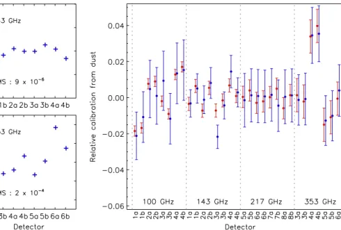
Fig. 13.Relative calibration measured by the dipole amplitude for each
polarization-sensitive detector with respect to the mean dipole across a frequency band.
level: D(`) < 10−4µK2 for CMB channels8; and D(`) ≈ 10−3µK2 for 353 GHz, except at ` = 2, where it reaches
10−2µK2. This demonstrates that the residuals of these system-atic effects have a negligible effect on τ measurements, except possibly at `= 2.
2.6.3. Inter-detector calibration of the polarization-sensitive bolometers
Calibration mismatches between detectors produce leakage of temperature to polarization. The inter-detector relative calibration of the PSBs within a frequency band can be tested on single-detector, temperature-only maps (the polarized signal of the full-frequency map is subtracted from the detector TOI). The best-fit solar dipole (determined from the 100 and 143-GHz full-frequency maps) is removed. The residual dipoles in the maps measure the relative calibration of each detector with respect to the average over the frequency band. The results are shown in Fig.13.
The low level of variations constrain the residual calibration mismatch between detectors that could lead to leakage of tem-perature to polarization. The relative calibration factors averaged over the full mission show rms dispersions of ±5 × 10⁻⁶ for
100 GHz, 9 × 10⁻⁶ for 143 GHz, 2 × 10⁻⁵ for 217 GHz, and 2 × 10⁻⁴ for 353 GHz. At 100 GHz, 143 GHz, and 217 GHz,
these dispersions are very small, and unprecedented for a CMB experiment. Absolute calibrations of band averages are dis-cussed in Sect.5.1. At CMB frequencies, results are still affected by gain errors between bands and by residual gain variations over time. At these frequencies, the gain mismatch is consistent with statistical errors (Tristram et al. 2011), therefore, it is not possi-ble to improve the gain mismatch any further at these frequen-cies. At 353 GHz, the gain mismatch is larger than the statistical errors. The worst outliers (bolometers 353-6a and 353-6b) also show large odd − even discrepancies in Fig.11. Therefore there is hope for improving the relative calibration.
8 Throughout this paper, we call CMB channels the 100, 143, and
217 GHz channels.
Fig. 14.Comparison of the response of each detector to dust as
mea-sured on the ground (blue) and as solved by SRoll (red).
2.6.4. Tests of bandpass mismatch leakage coefficients on gain: comparisons with ground tests
The SRoll mapmaking procedure (Appendix B) solves for temperature-to-polarization leakage resulting from the different response that each bolometer has to a foreground with an SED different from that of the CMB anisotropies. The solved band-pass mismatch coefficient associated with thermal dust emission is compared in Fig. 14to that expected from pre-launch mea-surements of the detector bandpass (Planck Collaboration IX 2014). The statistical uncertainties on the ground measurements are dominated by systematic effects in the measurements. For all bolometers except 143-3b, the two are consistent to within the error bars estimated using simulations. The smaller error bars are the sky determinations by SRoll and are in closer agree-ment with ground measureagree-ments than the conservative estimates of the systematic errors on the ground measurements would pre-dict. The only exception is bolometer 3b, for which the ground and sky measurements differ by nearly 3× the more accurate sky uncertainty.
2.6.5. Summary of improvements
The generalized destriper solution, solving simultaneously for bandpass-mismatch leakage, intercalibration errors, and ADC-induced gain variations and dipole distortions, has been shown to be necessary to achieve a nearly complete correction of the ADC non-linearities. This leads to much improved maps at low multipoles compared to previous releases. In Sect.6.2and AppendixBwe will demonstrate that SRoll mapmaking does not filter or affect the CMB signal itself.
At 100, 143, and 217 GHz, we are now close to being noise-limited on all angular scales, with small remaining systematic errors due to the empirical ADC corrections at the mapmak-ing level. These separate corrections should be integrated in the TOI/HPR processing for better correction. At 353 GHz, and to a lesser extent 217 GHz, we observe residual systematic cali-bration effects, as seen in Figs. 12 and13, but we will show in the following sections that the residuals are small enough to have negligible effect on the determination of τ. The origin of
this effect is not fully understood; correction algorithms are in development.
3. Consistency tests of the HFI polarization maps
As described above and in Appendix B, the SRoll mapmak-ing algorithm corrects simultaneously for several sources of temperature-to-polarization leakage that were not previously corrected.
Section3.2gives the results of null tests that show how sys-tematic effects at large angular scales are very significantly re-duced compared to those in the HFI polarization maps from the 2015 Planck data release. As a test of the accuracy of this process, the results are also compared with the HFI pre-2016 E2E simulations. We begin in the next sub-section (Sect.3.1) by showing that detection of the a posteriori cross-correlations of the final maps with leakage templates cannot work because of the degeneracy with the dipole distortion.
3.1. Temperature-to-polarization leakage
As discussed in Sect.2, any bandpass and calibration mismatch between bolometers induces temperature-to-polarization leak-age, and hence spurious polarization signals. Each leakage pat-tern on the sky for each bolometer is fully determined by the scanning strategy, along with a set of leakage coefficients, and the temperature maps involved (dipole and foregrounds). The SRoll approach improves on the 2013 and 2015 HFI map-making pipeline by correcting all temperature-to-polarization mismatches to levels where they are negligible. Detector inter-calibration has been much improved, as shown in Sect. 2.6.3. Similarly the residual bandpass leakage (mainly due to dust and CO) in the Q and U HFI pre-2016 maps is also greatly reduced (AppendixB.4.1).
In the 2015 data release, we used leakage template fitting (Planck Collaboration VIII 2016) to check a posteriori the level of temperature-to-polarization leakage residuals, although this leakage was not removed from the maps. From Sect. 2.6and the appendices, we expect temperature-to-polarization leakage to be very much reduced for the HFI pre-2016 data set. Contrary to expectations, however, the template-fitting test (expanded to account for synchrotron polarized emission) on the HFI pre-2016 release used in this paper still reveals significant leakage. Suspecting that the problem is residual dipole distortion induced by ADC non-linearity, which is not yet removed, we performed leakage tests on simulations both with and without the effect. This is done by forcing the gain to be constant within a point-ing period, which removes only the dipole distortion within the ADC non-linearity effects.
Figure15 shows that auto-spectra exhibit a leakage in the pre-2016 100-GHz data (green line), comparable to the simu-lations with (blue line) full ADC non-linearity effects. The red line, with the ADC dipole distortion effect removed, is lower by a factor of 5 or more. This demonstrates that the detected leak-age at 100 GHz contains a potentially significant, and possibly dominant, spurious detection due to a degeneracy between the dipole distortion and the leakage templates. This is in line with the low level of the leakage and the level of the dipole distortion discussed in Sect.2.5. This can only be confirmed through E2E simulations and comparison with data residuals from an appro-priate null test. The remaining systematic effects are at a level of 8 × 10⁻⁴µK2 for ` > 3. The quadrupole systematic term is an order of magnitude larger. As discussed before, quadrupole and
Fig. 15. Simulation of the template-fitting tests for
temperature-to-polarization leakage in the 100-GHz maps, with (blue) and without (red) ADC-non-linearity dipole distortion. The green curve shows the result of the leakage fit in the HFI pre-2016 data, which is comparable to the simulation with the ADC non-linearities. The red curve is lower by a factor of 5 or more, showing that dipole distortions due to ADC non-linearity are a significant contributor to the leakage. The black dashed line corresponds to the fiducial model F-EE with τ= 0.066.
octopole systematic effects dominate in Fig.9. The residuals of the ADC non-linearity dipole distortion at ` > 3 are small with respect to the F-EE signal.
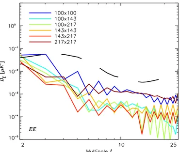
Figure16shows results for 100, 143, and 217-GHz data. All spectra show a rise similar to the one seen for the blue line in Fig.15, which simulates the ADC non-linearity dipole distor-tion at 100 GHz. The higher frequencies also exhibit negligible temperature-to-polarization leakage, but have comparable ADC non-linearity dipole distortions. This is a strong indication that, at these frequencies, the dominant residual systematic is also due to ADC non-linearity acting on the dipole, which is not removed from the maps, in agreement with Fig.17. This effect has to be accounted for in the likelihood before science results can be ex-tracted from the pre-2016 maps. The temperature-to-polarization leakage is at a level of 10−3µK2or lower at ` > 4. The dominant systematic at 353 GHz, in contrast, is calibration uncertainty (see Sect.2.6.3).
3.2. Null tests
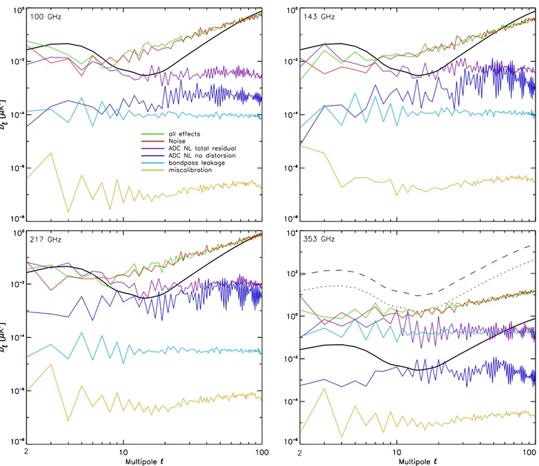
In this section we use null tests on power spectra, together with our understanding of the simulated systematic effects discussed in Appendix B, to demonstrate that we have identified all de-tectable systematic effects. In Fig. 17, the green lines show the total of noise and systematic effects. Noise (red lines) domi-nates at multipoles ` > 10 for all frequencies. For the CMB channels (100, 143, and 217 GHz) the main systematic is the ADC-non-linearity dipole distortion (purple lines), which is not removed in the mapmaking; for this systematic, it is not the residual but the effect itself that remains in the maps. The resid-uals from other effects of ADC non-linearities are smaller (dark blue lines), and the bandpass leakage residual (light blue) is smaller still. Frequency-band intercalibration residuals (orange) are even lower, as are other systematic effects that are not shown.
A&A 596, A107 (2016)
Fig. 16. EE auto- and cross-spectra of the global fit test of the
temperature-to-polarization leakage, for 100, 143, and 217 GHz. Levels are similar to that for 100 GHz, for which Fig.15shows that this is dom-inated by the ADC-non-linearity dipole distortion. The dashed black line corresponds to the fiducial model F-EE with τ= 0.066.
For the 353-GHz channel, which is used only to clean fore-ground dust, the simulated systematic effects at low multipoles are all negligible with respect to the F-EE model level scaled by the foreground correction coefficients for 100 and 143 GHz (dashed and dotted black). Although the inter-survey calibration difference shown in Fig.12is greater for 353 GHz than for the CMB channels, this does not affect the present results.
We perform null tests on four different data splits. The first is the odd − even survey differences. These map differences test residuals associated with the scanning direction and far side-lobes, short and long time constants in the bolometers, and beam asymmetry. The only clear evidence for any residual systematic effects associated with scanning direction is the odd − even solar dipole amplitude oscillation displayed in Fig.12. This is above the noise level only at 353 GHz (Sects.2.6.2and2.6.3). Other scanning-direction systematic effects are almost entirely elimi-nated by the SRoll mapmaking algorithm, and are not discussed further in this section.
The other three data splits used for null tests are by “det-set” (Planck Collaboration VII 2016), by the first and second halves of each stable pointing period (Planck Collaboration VII 2016), and by the first and second halves of the mission (Planck Collaboration VIII 2016). In each case, we compute C` spectra of the difference between the maps made with the two subsets of the data. The spectra are rescaled to the full data set. The re-sulting spectra contain noise and systematic errors, and can be compared with the FFP8 simulations (Planck Collaboration XII 2016) of the Planck sky signal and TOI noise only.
Detset differences are sensitive to errors in detector parame-ters, including polarization angle, cross-polar leakage, detector-mismatch leakage, far sidelobes, and time response.
Half-ring differences are sensitive to detector noise at levels predicted by the analysis of TOI (Sect. 2.3). All systematic er-rors cancel that are associated with different detector properties,
drifts on timescales longer than 30 min, and leakage patterns as-sociated with the scanning strategy9.
Half-mission differences are sensitive to long-term time drifts, especially those related to the position of the signal on the ADC and related changes of the 4-K lines affecting the mod-ulated signal.
The pre-2016 E2E simulations can be used to distinguish whether systematic effects are comparable to the level of the baseΛCDM EE spectrum and could therefore affect the τ de-termination, or whether the systematic effects are negligible or accurately corrected by SRoll.
Figure18compares EE auto-spectra of detset, half-mission, and half-ring null-test difference maps for the pre-2016 data and the 2015 release data. The half-ring null test results (blue lines) agree with FFP8 as expected. For detset (red lines) and half mis-sion (green lines) null tests, the 2015 data show large excesses over the FFP8 simulation up to ` = 100. In contrast, the HFI pre-2016 data detset differences for 100 and 143 GHz are in good agreement with the FFP8 reference simulation. This is no sur-prise as systematics detected by this test have been shown to be small. At 217 GHz, the detset test is not yet at the level of FFP8. For the half-mission null tests, the analysis of systematic ef-fects shows that the ADC-non-linearity dipole distortion, which has not been removed, dominates, and should leave an observ-able excess at low multipoles in this test, which is not however seen. Thus this null test does not agree with the systematic anal-ysis. A possible explanation is that the destriping is done on the full mission and applied to the two halves of the mission. The correlation thereby introduced in the two halves could lead to an underestimate of the residual seen in the null test. We checked this by constructing a set of maps in which the destriping is done independently for each half-mission. Figure19shows the results of this check. The independent destriper for the two half-missions (blue lines) shows a systematic effect at all frequencies in the half-mission null test that is not seen for the full mission minimization (red lines). The separated minimization can also be compared to the sum of all simulated effects (green lines); it shows the expected behaviour for the 100 to 217-GHz bands. We conclude that the uncorrected ADC-non-linearity dipole dis-tortion accounts for most of the systematic detected by this new half-mission null test. This, of course, does not imply that the maps should be constructed using the separate half-mission min-imizations because these use fewer redundancies than the full mission ones, and are therefore less powerful.
At 353 GHz, the null test is below the sum of all system-atic effects between multipoles 2 and 50, and is not catching all systematic effects. The calibration and transfer functions for 353 GHz are not captured by the half-mission null test; this can plausibly explain the difference.
We have shown that the destriping of the two half-missions should be done independently in order to detect ADC non-linearity residuals. The 2016 data release will therefore include half-mission SRoll fits of parameters.
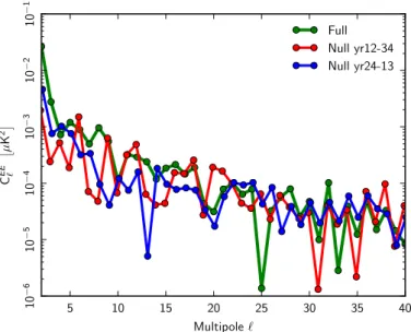
Figure20shows EE and BB spectra of the difference maps and cross-spectra (signal) over 43% of high latitude sky for both the 2015 HFI maps and for the HFI pre-2016 polarization maps described in this paper, and shows the relative improvements made by the SRoll processing. Differences between 2015 and
9 A small correlated noise component induced by the deglitching
pro-cedure and the TTF corrections leads to non-white noise spectra (as in Fig.1) different from the noise levels predicted from the TOI analysis
(Planck Collaboration VII 2016;Planck Collaboration VIII 2016). The
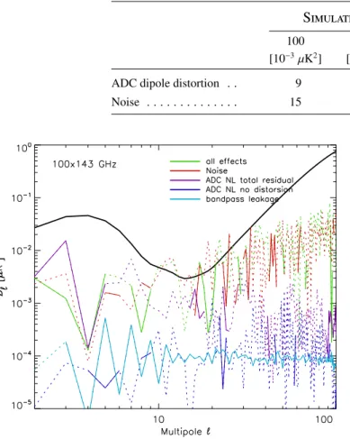
Fig. 17.Residual EE auto-power spectra of systematic effects from the HFI pre-2016 E2E simulations computed on 50% of the sky (colours
specified in the top left panel apply to all panels). The purple line (ADC NL total residual) shows the sum of all effects associated with ADC non-linearity. The dark blue line (ADC NL no distortion) shows the level without the dominant dipole distortion. The plots show also the F-EE model (black curves). The 100-GHz and 143-GHz model scaled to 353 GHz with a dust SED is shown as dashed and dotted lines, respectively.
pre-2016 power spectra are not particularly sensitive to the po-larization mask. The cross-spectra show the total signal level, dominated by polarized dust emission at ` <∼ 200 and, in EE, by the CMB at ` >∼ 200. This allows a direct comparison of the signal with noise plus systematic effects.
In Fig.20, the 353-GHz detset null test for the 2015 data (blue line) at 3 ≤ ` ≤ 55 is 30 times larger than the FFP8 noise, and is at a level larger than 10% of the dust foreground spectrum. In the 2015 data release, systematic effects in the 353-GHz maps constitute the main uncertainty in the removal of dust emission from 100 and 143 GHz at low multipoles, dominating over statis-tical uncertainty in the dust removal coefficient (around 3%, see Sect. 5.2). In the pre-2016 data detset differences (green line), the systematic effects are much lower, but not yet at the TOI noise level.
In summary, all known systematic residuals have been seen in at least one null test at the expected level. Conversely, there
is no excess over noise seen in a null test that is not accounted for by a known systematic. This important conclusion fulfills the goal of this section. However, one systematic effect has not been corrected at all, namely the ADC-induced dipole distortion be-cause it requires a better ADC model that can be applied at the TOI or ring level simultaneously with the correction of other sys-tematic effects. This will be done in the next generation of data.
4. LFI low-`polarization characterization
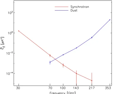
The measurement of τ for the Planck 2015 release was based on the LFI 70-GHz maps, cleaned of synchrotron and dust emission with 30-GHz and 353-GHz templates, respectively (Planck Collaboration XIII 2016). In this paper we use the 70, 100, and 143-GHz polarization maps to calculate 70 × 100 and 70×143 cross-spectra (see Sect.6). Since the LFI and HFI instru-ments are based on very different technologies, the systematic
A&A 596, A107 (2016)
Fig. 18.EEauto-power-spectra of detector-set, half-mission, and half-ring difference maps for 100, 143, and 217 GHz. C`rather than D`is plotted
here to emphasize low multipoles. Results from the Planck 2015 data release are on the left; results from the pre-2016 maps described in this paper are on the right. Colour-coding is the same for all frequencies. We also show for reference an average of FFP8 simulations boosted by 20% to fit the half-ring null tests. The black curves show the F-EE model.
effects they are subject to are largely independent. In particular, the dominant systematic effects in the two instruments (gain un-certainties for LFI and residual ADC effects for HFI) are not ex-pected to be correlated. Therefore LFI × HFI cross-spectra pro-vide a cross-check on the impact of certain systematic effects in the estimate of τ. There can be common mode systematics as well as chance correlations, however, so the cross-spectra cannot be assumed to be perfectly free of systematic effects.
In this analysis we use LFI data from the 2015 release. A de-tailed discussion of the systematic effects in those data is given inPlanck Collaboration III (2016). To assess the suitability of the LFI data for low-` polarization analysis, we analyse residual
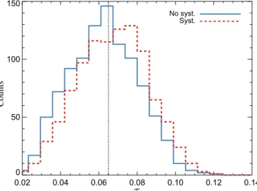
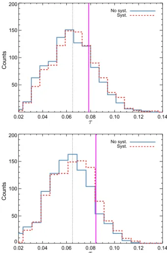
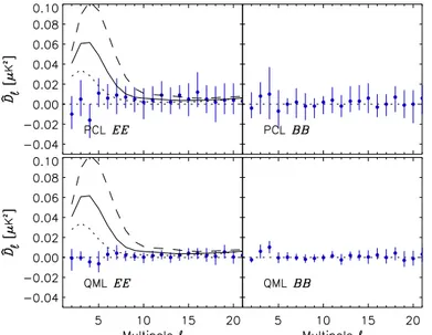
systematic effects in two ways, first using our model of all known instrumental effects (the “instrument-based” approach; Planck Collaboration III 2016), and second using null maps of mea-sured data as a representation of residual systematic effects (the “null-test-based” approach). In each case, we evaluate the im-pact of systematic effects on the extraction of τ by propagating them through foreground removal, power spectrum estimation, and parameter extraction (Fig.21). We then use our instrument-based simulations to support a cross-spectrum analysis between the LFI 70-GHz channel and the HFI 100- and 143-GHz chan-nels. A summary of the effects that are most relevant for the present analysis is given in AppendixC.
Fig. 19.EEand BB cross-power spectra of the residual effect computed from null tests between half-mission maps based on full mission mini-mization (red curve) or independent minimini-mization for each half mission (blue curve). This second approach clearly shows a systematic effect. The sum of all systematic effects, dominated by the ADC-non-linearity dipole distortion shown in green in Fig.17, is at the same level as the simulated null test with independent minimization. The FFP8 power spectrum is given again for reference.
A&A 596, A107 (2016)
Fig. 20.EEand BB spectra of the 2015 maps and the pre-2016 maps used in this work at 100, 143, 217, and 353 GHz. The cross-spectra of detset
and half-mission maps and the auto-spectra of the detset and half-mission difference maps are shown. The maps are masked so that 43% of the sky is used.