3D-printed sensor dynamical characterization

DELL’INFORMAZIONE

Laurea Magistrale in Ingegneria Meccanica

Supervisor: Prof. Emanuele ZAPPA

Alessandro BONANOMI

875701

Academic Year 2018/201

3D-PRINTED SENSOR DYNAMICAL

CHARACTERIZATION

Summary

1 Introduction ... 5

2 State of Art ... 6

2.1 Short Introduction about MEMS ... 6

2.2 3D Printed MEMS ... 6

2.3 Necessity of 3D Vision Systems for Measurements ... 7

2.4 Choice of the Measurement Technique ... 8

2.5 Fundamentals of Pose Estimation ... 8

2.5.1 Image formation ... 9

2.5.2 Basics of pose estimation ... 14

3 3D Printed MEMS Prototypes... 16

4 Implementation and validation of the 3D Measurements system ... 18

4.1 Measurement System ... 19

4.2 Binarization and Blob Analysis ... 22

4.3 Camera Calibration ... 23

4.4 Pose Estimation: implementation issues and solutions ... 26

4.5 From Camera Reference System to Sensor Reference System ... 27

4.6 Post-processing ... 29

4.7 FRF analysis ... 32

4.8 Static tests ... 34

5 Experimental results... 37

5.1 Preliminary Measurement Analysis (impulses) ... 37

5.1.1 Recording System Description ... 38

5.1.2 Camera Calibration ... 39

5.1.3 Preliminary Measurement Results ... 39

5.2 Shaker Measurements: set 1 ... 56

5.2.1 Recording Systems Description ... 56

5.2.2 Camera Calibration ... 58

5.2.3 Windowing ... 59

5.2.4 Set 1 Results ... 59

5.3 Shaker Measurements: set 2 ... 77

5.3.1 Camera Calibration ... 78

5.3.2 Set 2 Results ... 79

5.4 Critical analysis of the results of random and harmonic tests ... 85

6 Conclusions ... 88 7 Bibliography ... 89

1 Introduction

In this thesis I will present a study of the dynamical properties of a MEMS sensor produced by Additive Manufacturing (AM).

Today, this kind of sensors are widely used in many applications because they’re small and light so that they can be used in many devices and design issues in fact, industries specialized in semiconductors, are dominated by these silicon-based microelectromechanical systems technologies.

Due to the synchronous development of manufacturing technologies like 3D printing and integrated circuits it’s possible to make further researches about MEMS

technology area.

Now, even metallic materials can be easily printed starting from metal powder and small dimensions features and components can be designed and produced for a wide range of necessities. This possibility of creating small parts and characteristics led to a new generation of smart structures; in fact, these components’ features can be sensitive to the external environment and so used both as sensors for control and monitoring and as actuating devices.

In addition, a great advantage of AM is the possibility of manufacturing customized MEMS sensors in function of the final necessities and produce them in very small batches (at least one unit).

The research prospective is oriented on the design and the final manufacture of more and more small and customizable sensors in order to cover a wider as possible range of applications.

My work proposes a feasibility study of a metrology qualification system of these type of 3D printed sensors; the measuring technique is based on images acquisition and analysis made with the pose estimation technique.

Mechanical characterization is fundamental for their use, in fact this technique is able to track the six degrees of freedom motion of a rigid body in order to reconstruct its dynamics, as we will see in the followings.

In chapter 2 I will present the state of art of MEMS technology and the necessity of a vision measuring system coupled with the pose estimation technique for acquisition and processing.

In chapter 3 instead I show some design issues and simplifications adopted to theoretically study the sensor and extrapolate some analytical data in order to have an idea of the studied variables magnitudes.

Then, in the successive chapters 4 and 5 the measuring system and the obtained experimental results are explained in detail.

2 State of Art

2.1 Short Introduction about MEMS

MEMS stays for Micro Electro-Mechanical System because they’re devices in the scale of microns; this technology can be considered one of the most revolutionary of the 21st

century because it has changed dramatically the design of the electronics, informatics and mechanics especially in the field of electro-mechanical control and actuation. They are usually made of a microprocessor and several components that interact with the surroundings such as microsensors and actuators. Due to the high surface area to volume ratio of MEMS, forces produced by ambient and fluid dynamics are more important design features than with larger scale mechanical devices.

The fabrication of MEMS started from the evolution of process technology in semiconductors; the basic techniques are deposition of material layers, photolithography and etching to produce the required characteristics. The principal materials used for their fabrication are silicon, polymers, metals and ceramics.

Common commercial application of MEMS are: accelerometers (as we will see in the following), gyroscopes, pressure sensors, optical switching devices, microphones, magnetometers, ultrasound transducers, etc.

2.2 3D Printed MEMS

Today, MEMS inertial sensors are dominating the automotive field because of their continuous improvement in terms of dimension and power consumption.

Additive Manufacturing (AM) technologies, for example 3D printing, could be possible fabrication methods for these sensors because it is necessary only to design them starting from a CAD file.

Several kinds of accelerometers can be created passing through computer-aided design and then manufacturing but, for my work, I will concentrate the attention to single axis MEMS and particularly on a z-axis sensor whose aim is mainly sense the acceleration along the its out-of-plane direction.

The fabrication process of these kind of accelerometers is basically divided into 3 steps in order to obtain the desired characteristics [6]:

1) 3D printing:

z-axis accelerometers are SL-printed within 30 minutes with DL260® (DWS Systems) commercially available resin by exploiting a SL machine model DWS028JPlus characterized by 22μm (laser spot diameter) and 10μm of lateral and vertical resolution. SL-printed models are post-cured.

2) Wet-metallization:

a first electroless Cu layer of 0.5μm and a second 1.5μm layer of electrolytic Cu are deposited on the 3D-printed structures.

3) Two 100μm PET (Polyethylene Terephthalate) sheets are placed between the printed frame of the device and each of the two Cu sheets to provide electrical isolation and a 200-μm air gap between the proof mass and the Cu bases.

Figure 1: Physical model of the studied sensor (z-axes accelerometer)

(1)

(2) Where k is the stiffness of the two elongated springs, m is the entire mass of the accelerometer and ω is the natural frequency of the z-axis mode (Figure 1) which was estimated to be about 500 Hz thanks to laser measurements.

Obviously, z-axis mode is not the only one vibration mode of the sensor because it has a certain stiffness even in x and y axis, so we will take into consideration even the vibration along them [1].

2.3 Necessity of 3D Vision Systems for Measurements

As we can appreciate, the sensor is too small and light to estimate its natural frequencies and dynamical behavior using a classical accelerometer because it would change too much the mass of the sensor and the natural frequencies would be totally wrong.

Using this kind of contactless measurement, we don’t damage the sensor and we’ve a good reconstruction of the 6 degrees of freedom motion of the rotor in the space. There are many techniques in order to reconstruct the recorded motion of an object so it’s important to analyze as better as possible the problem from all its facets and establish the more appropriate technique of measurement and analysis.

𝑘Δ𝑧 = −𝑚𝑎

Δ𝑧 = −

𝑎

𝜔

The only drawback of adopting a vision system-based measurement is that it is not so easy to deal with the quantity of material to acquire (high number of frames) and the acquisition time too in fact, in order to characterize this kind of sensor, we need a high-speed camera because the vibrational frequencies are in the order of hundreds of hertz. Fortunately, today the devices processing power is very high, so this kind of problems are restrained to very accurate and precise measurement systems.

2.4 Choice of the Measurement Technique

In vision systems and measurements in order to obtain three-dimensional

information from image recordings is typical the use of stereoscopy which requires the use of more than one camera.

A stereoscopic measurement system it’s very difficult to set up because all the

cameras need to be focused and the lightening system must be set in the proper way. For my aim I thought about a smarter measuring technique which involves the use of a single camera and a processing software in order to manage the data acquired. I opted to the pose estimation technique which is the best one in this case because we can avoid the use of more than one camera, so prevent focus problems due to the fact that we can record on the orthogonal axis of the sensor and the lighting system is limited to the recording area and not so difficult to be set up.

Moreover, it’s simpler and faster than other 3D measurement techniques because in this case I have only to create a geometry characterized by some specific markers that are tracked by the pose estimation algorithm in order to reconstruct their motion and so extract further information, i.e. the dynamical response.

Then, the problem is managing the program and obtain results with a true physical manner because the input files for the pose estimation algorithm derives from the blob analysis which can find, during the process, some problems of blobs identification in certain frames.

The excitation step and its acquisition are crucial although the pose estimation could not be able to track the markers in the desired way; extremely small markers’ displacements, bad focus of the camera or not proper illumination are typical features that can affect this processing step.

For the analysis of the acquired frames I used two software implemented in LabVIEW: one for binarization and blob analysis in order to find the centroids’ centers of gravity and the other one is for the pose estimation in order to extrapolate their displacements and rotations.

2.5 Fundamentals of Pose Estimation

Pose estimation is a very useful and spread technique in machine vision systems because it allows to determine position and orientation of a calibrated camera from known 3D reference points and their images.

This technique it’s a powerful tool to estimate three-dimensional parameters of a rigid body which is the most important problem in motion analysis.

Its applications are very spread in scene analysis, motion prediction, robotic vision and online dynamic industrial processing (online control system) [11].

It’s important to distinguish two types of this technique, online and offline, that involve different computational effort and algorithms; basically, online methods are used in order to have instantaneous information about the system taken into consideration due to control issues and feedback necessities.

In order to provide an introduction to pose estimation techniques, it is necessary to present the image formation process.

2.5.1 Image formation

Let’s say something about the image formation process and focus about the pose estimation technique which is the inverse procedure (Figure 2).

Figure 2: Pose estimation technique is the inverse process of image generation Image formation is a process which allows to project an object in the tri-dimensional space in its corresponding bi-dimensional image; instead, it’s called vision the

opposite process with whom we can extract the extrinsic parameters (motion in the space for example) of an object starting from images.

So, in order to design vision algorithms like pose estimation it’s required to firstly develop a suitable model of image generation; this mathematical model has to be as manageable as possible because it has to be easily inverted for vision algorithms. I will consider two important mathematical approximations:

1. Thin lenses model: mathematical model defined by an axis (optical axis) and a plane perpendicular to it (focal plane) with a circular aperture centered at the optical center which is the intersection of the focal plane with the optical axis. Basically, adopting this model, diffraction and reflection are neglected and only refraction is taken into consideration.

Looking at the triangles in Figure 3 we can obtain the similarity relationships showed in the followings and then extract the fundamental equation of thin lenses:

Figure 3: Thin lens model: image of the point p is the point x of the intersection of rays going parallel to the optical axis and the ray through the optical center

We can find the similar triangles A and B: 𝒑 𝒙

=

𝒁

𝒛 (3)

and the similar triangles C and D:

𝒙 𝒑

=

𝒛−𝒇

𝒇 (4)

These two relationships lead to the following equation which is the fundamental equation of thin lens:

𝟏 𝒇

=

+

2. Ideal pin-hole camera model: if I let the aperture of a thin lens decrease to zero, all the light rays are forced to go through the optical center, and therefore they remain undeflected (the aperture of the cone decrease to zero, and the only points that contribute to the irradiance are the points x on a line through p).

If I let p have coordinates X=[X, Y, Z]T _{relative to a reference frame centered at the}

optical center, with the optical axis being the Z-axis, then it is immediate to see from Figure 4 that the coordinates of x and p are related by an ideal perspective projection:

:

Figure 4: Pin-hole camera model: image of the point p is the point x of the intersection of the ray going through the optical center o and an image plane at a distance f from the optical center Note that any other point one the line through p projects onto the same coordinates

[x, y]T _{(coordinates of the projected point x).}

Now, using this information, it is possible to build an ideal camera model taking into consideration the following relationships:

𝑿 = 𝑹𝑿_𝟎+ 𝑻 (7)

𝒙 = [𝒙_𝒚] =𝒇_𝒁[𝑿_𝒀] (8)

Where X defines the coordinate of p relative to a reference frame centered at the optical center, as I previously said, and the coordinates of the same point relative to the world frame by X0, which is also used to denote the coordinates of the point relative to the

initial location of the camera moving frame. Attaching a coordinate frame to the center of projection, with the optical axis aligned with the z-axis and adopting the ideal pin-hole camera model, the point p of coordinates X is projected onto the point of coordinates x (Figure 4). The two-dimensional reference frame in which x is expressed is called retinal image frame centered at the principal point with the axis x and y parallel to axis X and Y respectively and f is the focal length corresponding to the distance of the image plane from the center of projection.

Writing (8) in homogeneous coordinates:

𝒁 [𝒙𝒚 𝟏] = [ −𝒇 𝟎 𝟎 𝟎 −𝒇 𝟎 𝟎 𝟎 𝟏 𝟎 𝟎 𝟎] [ 𝑿 𝒀 𝒁 𝟏 ] (9)

Since the Z-coordinate (or the depth of the point p) is usually unknown, we may simply denote it as an arbitrary positive scalar 𝜆 ∈ ℝ₊.

Also notice that in the above equation we can decompose the matrix into:

[−𝒇𝟎 𝟎 𝟎 −𝒇 𝟎 𝟎 𝟎 𝟏 𝟎 𝟎 𝟎] = [ −𝒇 𝟎 𝟎 𝟎 −𝒇 𝟎 𝟎𝟎 𝟏] [ 𝟏 𝟎 𝟎 𝟎 𝟏 𝟎 𝟎 𝟎 𝟏 𝟎 𝟎 𝟎] (10)

Defining two matrices: 𝑨𝒇= [ −𝒇 𝟎 𝟎 𝟎 −𝒇 𝟎 𝟎𝟎 𝟏 ] ∈ ℝ𝟑𝒙𝟑 ₍₁₁₎ 𝑷 = [𝟏𝟎 𝟎 𝟎𝟏 𝟎 𝟎𝟎 𝟏 𝟎𝟎 𝟎 ] ∈ ℝ𝟑𝒙𝟒 ₍₁₂₎

from equation (7) we have that:

[ 𝑿 𝒀 𝒁 𝟏 ] = [𝑹 𝑻_{𝟎 𝟏}] [ 𝑿𝟎 𝒀𝟎 𝒁𝟎 𝟏 ] (13)

Combining the previous equations, the geometric model for and ideal camera can be described as: 𝝀 [𝒙𝒚 𝟏] = [ −𝒇 𝟎 𝟎 𝟎 −𝒇 𝟎 𝟎𝟎 𝟏 ] [𝟏𝟎 𝟎 𝟎𝟏 𝟎 𝟎𝟎 𝟏 𝟎𝟎 𝟎 ] [𝑹 𝑻 𝟎 𝟏] [ 𝑿𝟎 𝒀𝟎 𝒁𝟎 𝟏 ] (14) or in matrix form: 𝝀𝒙̃ = 𝑨𝒇𝑷𝑿̃ = 𝑨𝒇𝑷𝒈𝑿̃𝟎 (15)

The previous equation defines the projection of a generic 3D point p on the image plane

[x, y].

This ideal model is related to a very particular choice of reference frame, with Z-axis along the optical axis etc. In practice, when one captures images with a digital camera, the coordinates of the optical axis, the coordinates of the optical center and of the unit of measurements are not known.

The first step is defining the unit along x and y axes which will be defined in pixel using the scaling matrix S:

[𝒙𝒔 𝒚𝒔] = [ 𝒔_𝒙 𝟎 𝟎 𝒔𝒚] [ 𝒙 𝒚] (16)

Where 𝑠_𝑥 and 𝑠_𝑦 are the scale factors expressed in [pixels/mm] along the x and y directions. They are equal only when the pixel has a square shape, which occurs very often in cameras.

If the pixels are not rectangular, a more general form of the scaling matrix can be considered:

𝑺 = [𝒔_𝟎𝒙 𝒔_𝒔𝜽

where 𝑠_𝜃 is the skew factor and is proportional to cot 𝜃 of the angle between the image axes x and y; it represents the shape of the pixels and is equal to zero when the pixel is rectangular.

The coordinates 𝑥𝑠 and 𝑦𝑠 are defined with respect to the intersection point between

the optical axis Z and the image plane (which is the principal point with coordinates

(𝑜_𝑥, 𝑜_𝑦) ), therefore it is necessary to move the origin of the reference system which, by

convention, in images is in the top left corner: {𝒙_𝒚′′= 𝒙_{= 𝒚}𝒔+ 𝒐𝒙

𝒔+ 𝒐𝒚 (18)

Rewriting (18) in homogeneous coordinates, we obtain x’ that represents the image coordinates of point p in pixels:

𝒙′_{= [}𝒙′_𝒚′ 𝟏 ] = [ 𝒔𝒙 𝟎 𝟎 𝒔𝜽 𝒔𝒚 𝟎 𝒐𝒙 𝒐𝒚 𝟏] [ 𝒙 𝒚 𝟏] (19)

Combining (19) with the previously analyzed ideal model (14) I get the overall geometric model: 𝝀 [𝒙′𝒚′ 𝟏 ] = [ 𝒔𝒙 𝟎 𝟎 𝒔𝜽 𝒔𝒚 𝟎 𝒐𝒙 𝒐𝒚 𝟏] [ −𝒇 𝟎 𝟎 𝟎 −𝒇 𝟎 𝟎𝟎 𝟏] [ 𝟏 𝟎 𝟎 𝟎 𝟏 𝟎 𝟎 𝟎 𝟏 𝟎 𝟎 𝟎] [ 𝑿 𝒀 𝒁 𝟏 ] (20) or in matrix form: 𝝀𝒙̃′ = 𝑨_𝒔𝑨_𝒇𝑷𝑿̃ (21)

We can define the matrix 𝐴 = 𝐴𝑠𝐴𝑓 which is called intrinsic parameter matrix or

simply calibration matrix because it collects all the parameters that are intrinsic to the particular camera [9].

The information about matrix A can be obtained through the camera calibration process; I will focus on the procedure and on each parameter in chapter 4.3.

2.5.2 Basics of pose estimation

Until now, we are able to obtain the image coordinates in pixels starting from the position of the camera reference system and from the camera intrinsic parameters; now, the problem is inverting the previous matrix equation in order to perform the pose estimation.

Basically, the algorithm extracts the geometric primitives which allow to match the 2D points (obtained from the images) and the 3D points (previously determined on the object); this technique is very sensitive to the obtained images quality.

There are many techniques in order to solve the pose estimation problem which can be divided into two different families [4]:

1) Analytical methods; 2) Optimization methods;

The first ones are based on low number of points/lines and they have a finite set of solutions. Otherwise they’re characterized by low complexity, short computing time and solution accuracy in fact many solution techniques using 3 points were implemented: Dementhon and Davis’ three points based pose estimation technique [13], Fischler and Bolles’ RANSAC method [15], four to three points reduction methods , Quan and Lan’s linear methods [16], etc.

As regards the second family of solution techniques, a larger set of points has to be considered and a closed form solution do not exist for more than four points.

In order to obtain the solution, it is necessary to formulate pose estimation as a non-linear least-squares problem of a polynomial equation in image observables and pose parameters and solve it by non-linear optimization techniques (like Gauss-Newton method). The obtained solution is highly accurate, but the computing time is very long. Many of these kind of techniques were implemented: Kumar and Hanson’s iterative algorithm [12], Dementhon and Davis’ POSIT, Lu’s object-space collinearity error minimization problem [17], etc.

Adnan Ansar and Kostas Daniilidis, working on computer vision and augmented reality (AR), developed a real-time pose estimation application by which is possible to determine the pose starting from a small number of world objects that are points and lines.

Determining the pose is basically a process of error minimization characterized by nonlinear geometric constraints both on the image and on the target, so the existing algorithms are the classics gradient descent and Gauss-Newton methods [11].

Until now; I have focused only on the pose estimation solution technique, but it is also important the choice of the marker system because it has to be detected by a computer equipped by a camera and then passed to a tracking algorithm (pose estimation).

Figure 5: Example of markers used in computer vision and AR applications

Marker trackers used in computer vision are usually square or circular tags and their geometric primitives are well-detectable in images [14]: for my work I will consider simple geometries for pose estimation so there wouldn’t be problem in the primitives’ detection process.

For this analysis I used a software implemented in LabVIEW (National Instruments) by Politecnico di Milano which extracts the 3D motion of the reference points using as inputs their positions in each recorded frame (x and y coordinates in the 2D image reference system) and the camera calibration parameters.

After this process, we’ve obtained translations and rotations of the reference points in the camera reference system and so, in order to pass to the object reference system, geometric transformations are required (Chapter 4.5).

Despite the algorithm principle of operation, we can say that, for my work, pose estimation technique is smart and optimal because we’ve only to print a pattern of centroids and glue them to the sensor: 4 external centroids on the sensor’s stator (fixed part) and 4 internal centroids to the rotor (moving part).

3 3D Printed MEMS Prototypes

The sensor was thought to be light and smart but at the same time possible to be printed because very small geometries must be designed very well in order to obtain a good result from the selective laser melting process: a small variation of the thickness due to the fabrication process might change the natural frequency of the accelerometer. Mechanical design must be very precise because a well-designed accelerometer is sensitive only to the acceleration that we want to measure; in our case it’s the translational acceleration along z axis.

This process of minimizing or, if possible, eliminating other motion components along the interested one is called cross-axis sensitivity minimization.

As regard the analytical model, aluminum properties were considered in order to have an idea on which is the sensor’s theoretical natural frequency; in fact it’s considered as 1 degrees of freedom system with the most simple spring’s configuration (straight springs) and its entire mass concentrated in the central rotor (spring’s mass is considered negligible) The resulting stiffness can be calculated summing the two spring’s flexural stiffnesses along z-axis.

The structural parameters are: m = 0.00022162 kg l = 13 mm s = 0.6 mm t = 0.4 mm E = 70 GPa J = 1 12st3 [mm4]

From these we can obtain the total stiffness: k = 2 EJ

12l3 [

N m]

and then we can obtain a valued which gives us an idea of the vibrational frequencies order of magnitude (hundreds of hertz):

f = √k

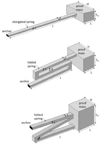
The configuration of the movable part shown in Figure 1 is not the only one designed in fact sensors with different spring’s geometries were printed in order to measure different frequency ranges (Figure 6 and Figure 7).

Figure 6: 3D printed sensors with different rotor’s stiffnesses

Figure 7: Schematic representation of the different rotor’s configurations These sensors, being built by Additive Manufacturing, can be made of complex features and very light and slender components; obviously, the feasibility is proportional to the state of art of 3D printing technology.

The mechanical characteristics of the desired features are strongly dependent of the machining parameters (porosity, irregularity, filling, etc…) and so the dynamical response will be affected. In addiction I must point out that even the resistance is touched by this manufacturing issues in fact a porosity can easily bring to a crack generation in the material followed by failure.

4 Implementation and validation of the 3D

Measurements system

I have to set a contactless measurement system based on a vision system made of a camera, an optics and an illumination set-up.

In order to track the 3 displacements and the 3 rotations (6 degrees of freedom) of the sensor’s movable part (rotor), whose aim will be measure inertial accelerations, I have printed a pattern of centroids with 2mm of diameter that has to be attached to the object and also a calibration pattern (basically, a chessboard) for the camera calibration.

Figure 8: Sensor used

The sensor taken into consideration for the analysis is 80x20x5 mm3 _{(Figure 8) and the}

area interested to the measurement is the area in neighbor of the centroids so it will result in a 30x20mm area of camera field of view which corresponds to 1200x700 pixels (circa).

We expect an out-of-plane vibrational motion in the order of tens of micrometers and a measurement uncertainty of 1μm as we know from previous analysis made on the object.

As said before I chose the pose estimation technique to extrapolate the 3D motion of the centroids after had binarized the images and identified the centroids.

The main steps of the analysis are: 1) Camera calibration;

2) Recording;

3) Binarization and blob analysis; 4) Pose estimation;

5) Post-processing (data extrapolation from pose estimation program and fitting); 6) Frequency analysis.

4.1 Measurement System

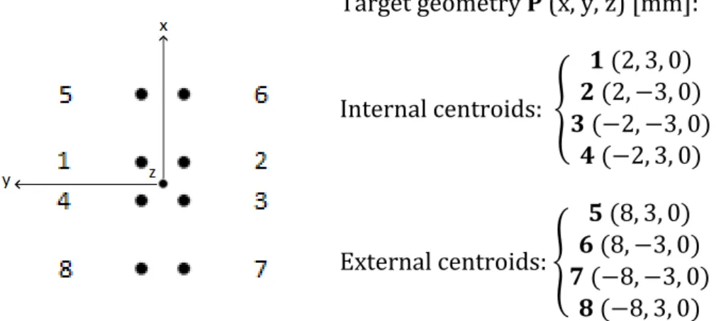
I chose a vision system in order to track the movement of a pattern made by 8 centroids: 4 attached to the rotor and the other 4 to the stator (Figure 9).

Figure 9: Centroids coordinates in the target reference system

The measurement system used was composed by a high-speed camera MIKROTRON EoSens mini2 with a ZEISS optics able to focus in an optimal way the centroids glued on the rotor and the rotor itself.

Target geometry P (x, y, z) [mm]: Internal centroids: { 𝟏 (2, 3, 0) 𝟐 (2, −3, 0) 𝟑 (−2, −3, 0) 𝟒 (−2, 3, 0) External centroids: { 𝟓 (8, 3, 0) 𝟔 (8, −3, 0) 𝟕 (−8, −3, 0) 𝟖 (−8, 3, 0)

Figure 10: High-speed camera mounted on the tripod

I set a powerful lighting system to permit the camera to distinguish the centroids because it records in black and white so, without a proper illumination, it is not possible to clearly identify the 8 blobs. The adopted lighting devices are Smart Vision Lights LED based illuminators.

Image recording is performed using the camera software MotionBLITZDirector2 (Figure 10) in which we can modify all the parameters for the acquisition such as shutter time, exposition time, field of view, frames per second, etc…

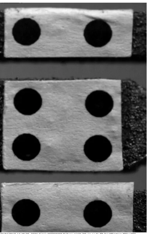
Setting the exposition time I can balance the light incoming the camera sensor and so starting to obtain a good focus; then balancing the shutter, which is the time in which the sensor is not acquiring in order to process the previous image obtained and send it to processing unit, I can increase or decrease the frame per second (fps) to acquire. We can perform this issue even decreasing the field of view of the camera as I’ve done for the recording; in fact, I have considered only the portion containing the 8 centroids minimizing as much as possible the field of view (Figure 11).

Figure 11: Adopting these field of view dimensions, I have recorded at 1500 fps;

In order to analyze the data obtained from the camera two programs for blob analysis and pose estimation were provided to me.

They’re both written with LabVIEW, so the results are not shown very well, especially for what concerns pose estimation, so I used MATLAB for the post-processing step of my work.

4.2 Binarization and Blob Analysis

This is the second step for the image processing because we must identify the centroids positions and track them image by image.

For this issue I used a software implemented in LabVIEW for binarization and blob analysis (Figure 12) which needs as inputs the image obtained by the camera and as output gives us for each image a .txt file in which are contained the positions in pixel of the centroids.

Figure 12: Program for blob analysis

Through 3 passages we can obtain a series of images clean of everything spurious in which there are only the 8 centroids.

These filtering passages are necessary because the software has to find the gravity center of each centroid so, if there’s at least another spurious centroid in the final image (right bottom of Figure 12), the software gives back a result which is not coherent with our analysis.

It’s important to verify that in almost all the frames is possible to identify each blob although we can come across problems of blobs identification that have serious repercussions in the pose estimation.

4.3 Camera Calibration

Calibration is a necessary step because allows us to estimate the intrinsic camera parameters, necessary to apply the pose estimation technique. Thanks to the pose estimation, it is possible to estimate the six degrees of freedom position of the target for each acquired image. This information, in turn, are fundamental to study the dynamic behavior of the 3D printed sensor.

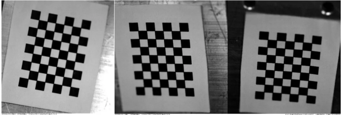
In order to perform the calibration of the camera I used the dedicated MATLAB Camera Calibration Toolbox which implements the Zhang camera calibration technique [2]. The camera calibration procedure requires a sequence of images of a planar chessboard. The calibration target has to be oriented with different

inclinations and perspectives to ensure a reliable estimation of the camera calibration parameters

Figure 13: Example of an acquired sequence of different orientations of the chessboard Once obtained these images (usually 15-20) they can be used by the toolbox to extract a MATLAB file containing all the information obtained by the calibration such as focal length, principal point, skew and distortion coefficients and uncertainties. First, the toolbox requires to the user the directory in which the images are located and then start to acquire them in memory.

Figure 14: Camera calibration toolbox main menu

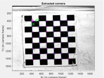
Then, from the principal menu (Figure 14), I can select the option ‘Extract grid corners’ in order to process all the images one by one selecting in each one the origin for the axis orientation and the other three corners (Figure 15).

In addiction we’ve to insert the values dX and dY which are the dimension of a single square of the chessboard.

Figure 15: Corners selection step

I’ve to perform this process many times as the number of the image taken for the calibration paying attention to the selection of the corners although the results at the end will be completely wrong.

Sometimes the toolbox, maybe due to a wrong interpretation the user’s selection of grid corner, is not able to count the squares along X and Y direction so I have to insert them manually.

Computing dX and dY for the first image then is valid for the following ones; the results of the grid extraction for first image are shown in Figure 16.

Figure 16: Projection of the grid generated from the selected corners

After the corner extraction of all the images the file calib_data.mat is generated: it contains the image coordinates, corresponding 3D grid coordinates, grid sizes, etc…

After this step we can perform the calibration from the toolbox menu and MATLAB gives back the following parameters (with even each uncertainty) as results:

• fC : focal length which indicates the distance, expressed in pixels, from the

camera sensor to the camera focal center and is stored in a 2x1 vector.

• Cc : principal point that is the point on the image plane onto which the perspective center is projected. It’s also the point from which the focal length of the lens is measured, and it’s stored in a 2x1 vector. I impose these two values extracting the information directly from the image in order to avoid uncertainties and obtain clearer camera intrinsic parameters;

• αC : skew coefficient which defines the angle between the x and y pixel axes (2D

image reference system) is stored in a scalar quantity. It’s almost zero in most of the cases because rectangular pixels are considered.

• kC : lens distortion coefficient (radial and tangential) that are stored in a 5x1

vector. The tangential component of distortion can often be discarded and so the last three components of the vector are almost zero (Zhang model). The vector has 5 components because the distorted image coordinates are calculated using a 5th _{order polynomia and so five coefficients are necessary.}

As example:

All these values are stored in vectorial variables and saved both in a .m and .mat file; notice that they’re given with the corresponding uncertainties.

Then we can reproject on the images the extracted corners clicking on and look at the reprojection error if we are interested or click on ‘Show Extrinsic’ in order to view the relative position of the grids in respect to the camera.

After this we click on ‘Recompensate corners’ in the principal menu and then, finally, run another calibration (in which no initialization and less iterations are necessary) in order to find the results; at the end MATLAB gives us a similar output to the previous calibration that we can save and use for the pose estimation procedure.

4.4 Pose Estimation: implementation issues and solutions

As said before, in order to perform the pose estimation, I used a software to calculate the time history of the sensor’s 6 degrees of freedom (Figure 17). In order to ease the data managing I used two similar programs: one for the four internal centroids (rotor’s centroids) and the other for the four external centroids (stator’s centroids).

Figure 17: Pose estimation software interface; the first page regards the input data and on the second one the results of the pose estimation are shown

The only one difference is geometrical because they have different coordinates with respect to the reference system of the software.

I had to face some problems about software initialization because, if I want to obtain reasonable results from this program, I have to set the START values as coherent as possible with the real starting position of the sensor’s motion time history with the respect to the camera sensor.

The starting position of the motion is not at 0 for all the axes as we can see from a test’s results in Fig but it’s relative to the camera reference system (Figure 18).

Figure 18: Camera reference system

For example, ‘tx’, which is the displacement along camera axes, differs from the real out-of-plane stator’s motion by the camera orientation angle and so, in order to obtain the desired motion components in the sensor’s reference system, I had to make a geometrical transformation as explained in the following chapter.

For what concern the achievement of a correct solution, I performed a continuous iteration in order to obtain a more and more reliable solution: this consists in running the program with reasonable starting values of the degrees of freedom, then, looking at the solution obtained, I chose as new starting values those near to the previous analysis settled ones. I performed this kind of iteration as many times as is necessary to obtain results as clean as possible from spurious data.

At the end of the pose estimation the results are stored and saved in .txt file which can be passed to MATLAB in order to better manage the data and perform a deeper

analysis.

4.5 From Camera Reference System to Sensor Reference System

Once obtained the results from pose estimation I passed them to a MATLAB program able to shifts all the variables time histories’ starting point down to zero which is the real physical situation (rest condition) and then pass from camera to target reference system (Figure 19) through a homogeneous transformation.

In order words, as output of the pose estimation I have the internal and external centroids 6 degrees of freedom motion in camera reference system shown in Figure 18 so I need a mathematic tool in order to pass to the sensor reference system shown in Figure 20in order to proceed for the analysis.

These transformations are based on projective geometry which deals with plane figures that are the projection of 3D object on a plane that is our eyes’ plane. The tools used to describe the points of projective geometry are the homogeneous coordinates, widely used in the digital field to represent objects and their motion. We start from a 3D motion of a 3D object in the space so the vectorial space is identified with R3 _{of the (x, y, z) ordered triad (cartesian reference system).}

A cartesian coordinate point (x, y, z) has as homogeneous coordinates any quaternity (X, Y, Z, W) of R4 _{such that W≠0, X/W=x, Y/W=y and Z/W=z.}

So (x, y, z, 1) and any other multiple (mx, my, mz, m) are homogeneous coordinates of the same point (x, y, z) of the space.

A ‘point’ with homogeneous coordinates (not all null) doesn’t correspond to a point in the tridimensional space but represents a point in the infinite direction of the

tridimensional vector (X, Y, Z). All of the not null quaternity (X, Y, Z, W) constitutes the projective tridimensional space P3_.

The centroids motion is a roto-translational motion, so I have to take into consideration the roto-translation matrix H which is represented as a

composition of rotational and translational motion and so a general rigid motion of an object (conservation of lengths and shapes must be taken into consideration):

𝑯 = [ 𝒏𝒙 𝒐𝒙 𝒂𝒙 𝒑𝒙 𝒏𝒚 𝒐𝒚 𝒂𝒚 𝒑𝒚 𝒏𝒛 𝒐𝒛 𝒂𝒛 𝒑𝒛 𝟎 𝟎 𝟎 𝟏 ] (22)

Where the first three columns represent the versors of axes X, Y, Z and the last one the origin of the reference system.

As regards the rotation, for this analysis I’ve taken into consideration the Euler angles representation in terms of roll (rotation around z-axis, Rz), pitch (rotation around y-axis, Ry) and yaw (rotation around x-y-axis, Rx).

Figure 19: From camera reference system to target reference system

This program generates two .mat files that contain rotations and displacements in the sensor’s reference frame; these files can be used after in order to manage the data and perform frequency analysis.

4.6 Post-processing

In order to visualize better the results, I used a MATLAB program which extracts the variables from the couple of .mat file and plots the time histories of the 6 degrees of freedom.

During pose estimation step it’s easy to find some spikes in the variables’ time histories due to some errors made by the program managing blobs’ positions obtained by the blob analysis.

In order to solve this problem, I made a portion of MATLAB code in which I used the command ‘csaps’ from the Curve Fitting Toolbox in order to fit the data with a spline in order to eliminate spurious data.

For example, let’s consider the variable ‘Ty’ of the internal centroids obtained from pose estimation:

Figure 21: Dirty signal

As we can see there are many spikes along data’s time history. Now I try to fit the curve with a spline superposing them in order to see the difference:

Figure 22: Fitted and dirty signals superposed

Fitting is not sufficient to eliminate the main spikes present in the signal so it’s necessary to make an average through the entire time history.

I chose to make an average through a ‘for’ cycle at each time instant of the previous and the next value of signal; the only problem that may income is the fact that is possible to have to consequent spikes and so we are not able to eliminate the spike. The result after the average now is cleaner and we can see the difference:

Figure 24: Clean signal

It can be noticed that some little spikes and a big one remains in the time history but it’s not important because they don’t give contribute to the frequency analysis which is the most important step (because those components have not periodicity).

The entire structure of all the measurement process is summarized in the following flow chart:

Figure 25: Flow chart of the acquisition and processing procedure

4.7 FRF analysis

After had ‘cleaned’ all the degrees of freedom time histories the frequency analysis can be performed using the ‘fft’ MATLAB function which implements the Fast Fourier Transform (FFT) allowing us to recognize all the sensor’s vibrational frequency components.

After had obtained all the spectra I computed the Frequency Response Function for all degrees of freedom considering as forcing term (input to the system) the vibration of the external centroids.

In fact, we can see the external motion as a constraint displacement because, for the tests, I attached the stator to ground and the rotor was free to vibrate due to inertial forces.

To reduce the effect of the noise in the measurements, the transfer function has been estimated with the estimators H1 and H2 [7], defined as:

𝑯_𝟏(𝒇) =𝑺̂𝑨𝑩(𝒇)

𝑺̂𝑨𝑨(𝒇) (23)

𝑯_𝟐(𝒇) =𝑺̂𝑩𝑩(𝒇)

𝑺̂𝑩𝑨(𝒇) (24)

These two estimators are used in order to clean the signal from noises on the input (H2) and on the output (H1) and obtain reliable transfer functrions.

Signal A is defined as the generic degree of freedom (Tx, Ty, Tz, Rx, Ry, Rz) of the external part of the sensor (input signal) and B as the generic degree of freedom of the internal part (output signal).

The cross-spectrum 𝑆̂_𝐵𝐴(𝑓) between B and A is defined as the multiplication of the complex conjugate spectrum of B by the spectrum of A:

𝑺̂𝑩𝑨(𝒇) = 𝑩∗(𝒇) ∙ 𝑨(𝒇) (25)

and the cross spectrum 𝑆̂_𝐴𝐵(𝑓) between A and B is:

𝑺̂𝑨𝑩(𝒇) = 𝑨∗(𝒇) ∙ 𝑩(𝒇) (26)

Thus, its amplitude is the product of the two amplitudes, and phase the difference of the two phases.

The auto-spectrum 𝑆̂𝐴𝐴(𝑓) of the signal A is defined as the multiplication of the

complex conjugate spectrum of A by the spectrum of A:

𝑺̂𝑨𝑨(𝒇) = 𝑨∗(𝒇) ∙ 𝑨(𝒇) (27)

And the auto-spectrum of B:

𝑺̂𝑩𝑩(𝒇) = 𝑩∗(𝒇) ∙ 𝑩(𝒇) (28)

In this way the amplitude is the product of the two amplitude and the phase is the difference between them as before.

All the spectra are obtained after averaging all time histories recorded in order to minimize the noise present on the measurement; in fact, averaging, it is possible to highly reduce the presence of spurious components and so obtain cleaner spectra. In order to compute the FRFs I used the function ‘tfestimate’ which allows to estimate, as default, the transfer function with the H1 estimator.

Every time history is composed of N points depending on the sampling frequency adopted and the ‘tfestimate’ function allows to automatically split the time history of the input and output in K sub records with M samples each and these sub records can be extracted with a custom overlap of P points.

4.8 Static tests

In order to verify the correct functioning of the entire measurement system some quasi-static tests on a micrometric slope were performed.

Practically, if the sensor is translated of a quantity X [mm] perfectly along x-axis for example, I expect that the pose estimation algorithm returns me the same value of displacement along that axis.

As results, I obtained a correct estimation of the degrees of freedom motion along the axes perpendicular to camera axis (displacement Tx and Ty) and on the rotation around z-axis (Rz).

For the other degrees of freedom Rx, Ry and Tz the uncertainty is one order of magnitude higher because the camera has more difficulties in tracking out-of-plane small displacements and rotations.

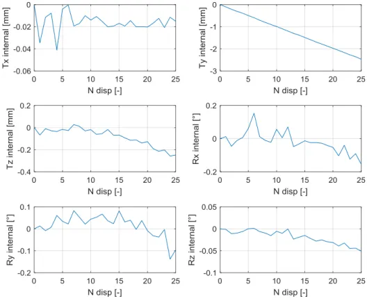
In the followings I will show the results obtained performing 25 displacement of 0.1mm mainly along y direction: I expect to obtain values of the rotations near to zero and even for the translations except for Ty.

I must underline the fact that the uncertainty about the displacement on the

micrometric slope is not negligible with respect to the measurement technique, so the procedure that I'm performing is only to verify the correct functioning of the

measurements made by the vision system with the imposed displacement.

The measurement resolution r of the slope is 0.5μm and I can obtain the instrument uncertainty u (type B) with the expression 𝑟

2√3 and I obtain a value of 2.9μm. I will consider only the internal centroids for the uncertainty estimation, and the results are shown in Figure 26:

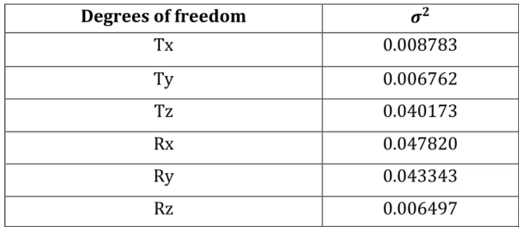
In order to understand the uncertainty of measurement, I computed the standard deviation of the different degrees of freedom and the results are shown in the following table:

Table 1: Standard deviations of the degrees of freedom related to the internal centroids

Degrees of freedom 𝝈𝟐 Tx 0.008783 Ty 0.006762 Tz 0.040173 Rx 0.047820 Ry 0.043343 Rz 0.006497

For simplicity of representation, in Table 1, I neglected to write the measurement unit, but it must be underlined that the standard deviation has the same unit of the analyzed data (millimeters for translations and degrees for rotations).

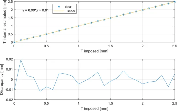
As I previously said, the uncertainties of Tx, Ty and Rz are one order of magnitude lower rather than the other degrees of freedom due to the measurement system characteristics (camera has more difficulties in tracking motions in the same direction of the camera axis). Finally, I plotted the estimated total translation (obtained computing the quadrature of Tx, Ty and Tz) and the discrepancies with respect to the linear trend, in function of the imposed displacement of the

micrometric slope:

Figure 28: Total internal translation and discrepancy in function of the imposed displacement The linear trend fits very well the analyzed displacement with a very low error (1% for the total internal translation) so the camera is tracking in the proper way the movement. In order to have further information, I computed the correlation coefficients of both the data sets:

Table 2: Correlation coefficients

Total translations 𝒓𝟐

Total external translation 1

Total internal translation 1

In fact, the correlation coefficients have value equal to 1 and this means that the trend is perfectly linear.

Now, it’s possible to perform some experimental test because I have verified that the algorithm is able to track in the proper way the centroids centers of gravity with a very low percentage of error.

5 Experimental results

5.1 Preliminary Measurement Analysis (impulses)

For these first tests I considered the use of a normal and a rubber-covered beam to produce different impulses on the table in order to excite the sensor, attached to the table by the stator, and in particular to excite the rotor (relative motion between movable and fixed part of the object) which is the sensor’s part used for the measurements in a common MEMS.

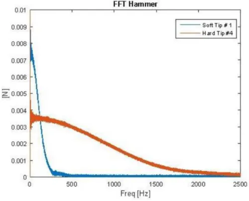
The beam tip is a mechanical filter in fact determines the excited bandwidth and so the cut-off frequency to be chosen for the analysis as we can see from Figure 29.

Figure 29: Example of the difference between a soft and a hard tip on a dynamometric hammer However, I decided to show only the results obtained by using the normal beam (hard tip) in order to excite the sensor for a wider as possible bandwidth.

So, after the camera calibration, I have performed two tests which were only to have an idea of the natural frequencies of the system: the first one was made performing only one beat on the table and sampling at 1500fps and in the second one I beat more than one time and acquired at 1850fps in order to increase the frequency resolution. However, these are only preliminary tests whose aim is only to give us a general idea about amplitudes and frequencies of vibrations and to verify the measurement system’s reliability.

I put in evidence the fact that a failure process is undergoing in the sensor because the two opposite strips that link rotor and stator are strongly sensitive to fatigue damaging during testing, so the results won’t be totally reliable because of the change in mechanical properties.

5.1.1 Recording System Description

As said before I used a powerful high-speed camera coupled with an optics able to well focus the centroids on the sensor. Moreover, I used only a couple of strong LED lights because it’s necessary to distinguish the centroids from possible shadows present in the room although blob analysis will be completely wrong.

5.1.2 Camera Calibration

For this issue I’ve used a classical chessboard made by 3x3 mm squares (Figure 15)using the same field of view that I will user for the following acquisition (although the calibration is wrong).

The uncertainties given in the followings and even in the next tests performed are different from the standards imposed by regulations because they’re output of the MATLAB calibration.

The output of the camera calibration obtained from MATLAB is:

fC = [19391.2; 19347.1]

Cc = [847 ; 854]

αC = 0.0 (imposed equal to zero, as described in Chapter 4.3)

kC = [-0.823 ; 0.0 ; -0.0 ; -0.0 ; 0,0]

And I report even the uncertainties of each parameter:

fC _error = [2097.4 ; 2116.5]

Cc _error = [0.0 ; 0.0]

αC _error = 0.0 (imposed value)

kC _error = [1 ; 0.0 ; 0.0 ; 0.0 ; 0.0]

5.1.3 Preliminary Measurement Results

• TEST 1:

For the starting test, as I previously said, I performed one beat on the table and acquired at 1500Hz.

It is very important to excite the structure as correctly as possible the structure avoiding ‘double hits’ although the single impulse response is not totally reliable (the structure has no time to show all its mode of vibration).

Time domain analysis:

In Figure 32 and in Figure 33 displacements and rotations along the 6 degrees of freedom are shown for both the internal and the external centroids.

Figure 32: Displacements along x, y and z axes during the preliminary test 1

As we can see the average value of the vibrations of external and internal centroids is quite the same but, obviously, the amplitude and the frequency of vibration are different.

Figure 33: Rotations around x, y and z axes during the preliminary test 1

I must point out that before the impulse (system in rest position) the standard deviation of Rx and Ry is of the order of 0.1°, while it is of the order of 0.01° for Rz. This difference is sign of the different values of uncertainty on each degree of freedom and characterize the measuring technique.

In fact, having the camera axis almost parallel to z-axis, rotations around this axis generate a significative variation of centroids position on the acquired frames.

For this reason, the measuring system has lower uncertainty in Rz estimation rather than in Rx and Ry as I showed in the static tests in Chapter 4.8.

Frequency domain analysis:

For this kind of analysis, it’s not necessary to make the Fast Fourier Transform (FFT) of all the time history, since in the portion of the data before the impulse application and also in the end of the acquisition the vibration level is negligible, therefore these portions of data simply increase the noise level, without adding any information. Therefore, only the portion of the time histories between 0.9 and 2 s are considered in the frequency analysis.

Figure 34: Spectra of the displacements along x, y and z axes

The vibratory phenomenon is well shown in Figure 34 in fact it’s very easy to see that the constrained motion frequency is common for both the rotor and the stator (with different amplitudes) and these components are followed, in this case, by harmonics which are the vibrational linear frequencies of the rotor along the different axes. The same frequency component in the neighborhood of 140Hz can be easily found both in Ty and in Tz; however, there is another very important component in common at 240Hz which is very much evident in Tx spectrum but can also be linked to the small one in Ty plot and to the small group of frequency peaks near 200-250Hz in the Tz spectrum (the uncertainty on measurements brings to leakage).

Other not less important resonances can be found near 630Hz for Tx and near 500Hz for Ty.

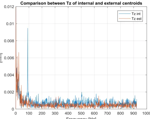
Even from the spectrum of Tz we can understand that the estimation of the out-of-plane motion is more difficult than the other two because of the presence of a more accentuated noise carpet.

Figure 35: Spectra of the rotations around x, y and z axes

In Rx and Ry there’s the common frequency component at 140Hz but Rz shows a new clear one at 350Hz.

The noise level in Rz spectrum is one order of magnitude lower rather than in the other two: this is due to the measuring technique as I previously anticipated.

Figure 36: FRFs of the displacements along x, y and z axes

We can extrapolate that the main frequency components as ratio between output and input are near 240Hz for Tx and Ty and near 140Hz for Tz and Ty.

Even from the Frequency Response Functions spectrum of Tz we can appreciate the higher amplitude of the noise carpet generated by the uncertainty on measurements. In these plots the Tx resonance near 620Hz and the Tz one near 500Hz are more visible.

Figure 37: FRFs of the rotations around x, y and z axes

As regards the rotational degrees of freedom, the most amplified one is the rotation around the out-of-plane axis. This fact, as well as it is less affected by measurement uncertainty, makes sense to the strong dynamical amplification regarding Tx and shows that this kind of geometry, if not perfectly excited along z-axis presents a strong translational effect.

• TEST 2:

In this following test I adopt the same type of excitation, but I performed more than one beat on the table in order to excite the structure more than before.

In addition, I started to acquire at 1850Hz and the recording is a bit longer.

However, even in this case, for the frequency analysis I chose only a significant part of the signal which is cleaner and so the frequency components are easier to be identified. I will proceed directly with the Frequency analysis because the time histories trend is the same as before.

Figure 38: Spectrum of the displacements along x, y and z axes in the preliminary test 2 We can observe that the resonances found in test 1 are present even in this but there’s something new in the frequency resolution and in the power distribution in fact for Ty now we’ve an accentuated resonance peak at 500Hz while before it was small and partially covered by noise.

The resonances at 140Hz previously found in Ty and Tz now are very clear and shifted in the neighborhood of 100Hz.

Figure 39: Spectrum of the rotations around x, y and z axes in the preliminary test 2 As regards Rx, the spectrum is quite the same but now the resonances near 100Hz and 500Hz are more visible even if for Ry is present a high level of noise on measurements. Rz shows a new resonance at 700Hz and the same small peak as before at 240Hz.

5.2 Shaker Measurements: set 1

The final test was performed using a shaker in order to induce controlled vibrations to the sensor and search for resonances in order to try to obtain its natural

frequencies of vibration.

Were necessary even a function generator and an amplifier linked to the shaker in order to generate desired excitations moduling amplitude and frequency of the wave; First, I opted to random signals because it’s necessary to excite all the frequency spectrum of the sensor in order to find the resonances.

Once detected the resonances I decided to generate sinusoidal functions with the same frequencies of the resonances previously found and then looked to the spectra obtained.

The aim is concentrating all the excitation signal energy along a certain frequency components looking for resonance amplitudes and possible non-linearities.

Practically, knowing the neighborhood of the resonance frequencies from the random test’s spectra, I modulated the input wave’s frequency with the function generator until had found the amplitude amplification due to each resonance.

5.2.1 Recording Systems Description

First, I linked the sensor to the shaker structure with to two thin plates and four bolts: the stator of the sensor must have the same motion of the shaker (rigid motion) so the rotor will be excited prevalently by the inertial forces Figure 42.

Figure 42: Electromagnetic shaker used for set 1 with sensor prototype equipped with the target on the rotor (internal centroids) and on the frame (external centroids)

The shaker was connected to the function generator able to produce both random and sinusoidal excitation which is linked to amplifier in order to modulate the gain and so the amplitude of the excitation.

The recording system is quite the same as the preliminary tests, but I decided even to assemble a sustaining structure for the lights in order to have a good resolution for the camera.

In Figure 43 we can see all the measurement chain in which are present:

1) Mikrotron EoSens mini2 high-speed camera with ZEISS optics mounted on the tripod with its connectors for power and data transfer;

2) Electromagnetic shaker by Ling Dynamic Systems (LDS) V400 Series which is a wide frequency band electro-dynamic transducer capable of producing a sine vector force till 196N (when force cooled); this type of vibrators is widely used in educational and research establishments to investigate the dynamic

behavior of structure and materials (fatigue and resonance testing for example);

3) Sensor mounted on the shaker (can’t be seen due to the strong light); 4) Function generator in order to generate the desired set point of vibration; 5) Amplifier connected to the function generator in order to set the proportional

gain for the input excitation;

6) Lighting system composed by two high power LED lights by Smart Vision Lights model SC75-WHI-W 75mm Low Cost Spot Light Colour: white and Wide Lens option;

7) Two articulated lamps;

8) Supporting structure for the lighting system.

5.2.2 Camera Calibration

Even for this test I chose a chessboard of 3x3 mm squares (Figure 44) because it is optimal for the camera frame dimensions. I changed only the plane on which the pattern is glued in order to have a surface more planar as possible.

Figure 44: Calibration pattern for the final tests The output of the camera calibration obtained from MATLAB is:

fC = [18793.5 ; 18844.2]

Cc = [847 ; 854]

αC = 0.0 (imposed equal to zero, as described in Chapter 4.3

kC = [0.01 ; 358.8 ; 0.0 ; 0.0 ; 0.0]

And the uncertainties of each parameter are:

fC _error = [663.5 ; 673.0]

Cc _error = [0.0 ; 0.0]

αC _error = 0.0 (imposed value)

kC _error = [1.6 ; 729.9 ; 0.0 ; 0.0 ; 0.0]

In order to obtain reliable results, I verified the first calibration with another final one and I observed that the results are the same so my first calibration was right.

5.2.3 Windowing

For these more accurate tests I used a Hanning window (Figure 45) in order to reduce the leakage of the acquired data and to obtain a higher resolution for the analysis of low damped vibrational modes.

Figure 45: Example of Hanning window

This is due to the fact that I cannot acquire a huge number of images although I couldn’t be able to manage all the amount of data so it’s sufficient to have a short-recorded time history and then apply the window to the FRF computation in order to limit the leakage effect shifting to the frequency domain.

As we can appreciate in the following analysis, the resonance peaks are very sharp, so we must have a good frequency resolution in order to correctly represent their

amplitude without power dispersion among the nearest frequencies. 5.2.4 Set 1 Results

As said before, I distinguished two types of excitation that are random and sinusoidal so, in this section, first, I will show and compare the results obtained by random inputs and then by sinusoidal ones.

Random excitations:

This type of signal, even called white noise, is theoretically able to excite all the frequency spectrum of an object so, for resonances detection, is the first useful tool. I made two random tests applying the same amplitude of 4Vpp but different gain values in order to appreciate vibrations on the sensor; for the first I set a value of 2 and then of 10 but this doesn’t mean that the amplitude of the last will be 5 times higher.

Let’s see the results obtained from the ergodic signal with gain equal to 2 acquiring with a sampling frequency of 2300Hz.

Figure 46: Displacements along x, y and z axes in the random test of set 1 As I know from the preliminary tests the two main vibrational modes of rotor are on the transversal direction (y axis) and the out-of-plane direction (z axis) in fact, the internal centroids have almost twice the amplitude rather than the external ones.

Frequency domain analysis:

Figure 48: Spectrum of the displacement along x-axis with gain equal to 2 and gain equal to 10 As I previously underlined, this property is common for all the degrees of freedom and ensure us that, amplifying the input, we don’t run into non-linearities, but we obtain only a higher amplitude of vibration.

Figure 49: Spectrum of the displacements along y and z axes

All the 3 degrees of freedom have a strong resonance in the neighbor of 290Hz and two smaller ones near 100Hz and 190Hz; Ty has even a small amplitude amplification near 580Hz.

As for what concern Tx, the other 2 degrees of freedom excited with gain equal to 10, present higher resonance amplitude at the same frequencies of those excited with gain equal to 2.

It can be noticed that the resonance peak at 100Hz it’s the same found in the preliminary impulse tests.

Figure 50: Spectrum of the rotations around x, y and z axes

The 290Hz component in Rx spectrum is meaningful because we obtained a resonance at the same frequency for Tz and, observing the geometry and the conventions, we can clearly understand the link between the two degrees of freedom.

Ry presents resonances at high frequencies in addition to the one at 290Hz, maybe because is a more constrained motion rather than Rx.

This high frequency components are the same found in the preliminary test but now the amplitude is lower because with the random input we try to spread the input power over all the possible frequencies.

As for Ry, being a more constrained motion, for Rz we can appreciate resonances at higher frequencies but this time we haven’t the 290Hz peak anymore.

Components at 100Hz and at 190Hz are still present but probably the energy is not correctly distributed in that frequency range (leakage around th peaks); in addition, as regards the 3 rotational degrees of freedom, the resonance in the neighborhood of 100Hz is characteristic both for the external and internal centroids.

Figure 51: FRFs of the displacements around x, y and z axes

From the FRFs plots it’s easy to observe that the resonance at 290Hz is common in all the three translational degrees of freedom with a substantial dynamical amplification.

Figure 52: FRFs of the rotations around x, y and z axes

In the next part of the analysis, I will excite the structure with sinusoidal signals having frequency value belonging to that bands of interests.

Sinusoidal excitations:

I will consider the 93.2Hz sinusoidal excitation (4Vpp and amplified with G=2) comparing the out-of-plane axis degrees of freedom with the ones excited at 210Hz which is the nearer one to the resonance peak detected in the random analysis

Figure 53: Displacements along x, y and z axes in the set 1 sinusoidal test (93.2Hz) For Tx and Ty, the relative motion is very strong but, as we can appreciate from the following graph, there’s isn’t a relative motion between internal and external centroids along z-axis.

This means that, for this range of frequency, I excited only a transversal mode of vibration for the sensor; let’s see the difference between the 93.2Hz and the 210Hz sinusoidal excitations.

From this previous plot we can deduce that at 93.2Hz the out-of-plane dynamical amplification is near to zero so the FRF at this frequency will assume a value near to 1. Let’s see what happens to Tz when excited at 210Hz:

Figure 54: Displacements along z-axis in the set 1 sinusoidal test (210Hz)

Now the relative motion is really evident and also the various harmonics of the rotor motion that can be easily found in the Tz spectra.