A comparison among deep learning techniques in an autonomous driving context

(1)

ALMA MATER STUDIORUM

UNIVERSITÀ DEGLI STUDI DI BOLOGNA

Scuola di Ingegneria e Architettura di Cesena

Corso di Laurea Magistrale in Ingegneria e Scienze Informatiche

A COMPARISON AMONG DEEP LEARNING

TECHNIQUES IN AN AUTONOMOUS DRIVING

CONTEXT

Elaborata nel corso di: Sistemi Intelligenti Robotici

Tesi di Laurea di:

LUCA SANTONASTASI

Relatore:

Prof. ANDREA ROLI

ANNO ACCADEMICO 2016-2017

SESSIONE II

(2)

(3)

KEYWORDS

Autonomous Driving Deep Learning Reinforcement Learning

(4)

(5)

Whenever I hear people saying AI is going to hurt

people in the future I think, yeah, technology can

generally always be used for good and bad and you

need to be careful about how you build it. If you’re

arguing against AI then you’re arguing against safer

cars that aren’t going to have accidents, and you’re

arguing against being able to better diagnose people

when they’re sick.

[

M. Zuckerberg ]

(6)

(7)

Introduction

The recent advances in computational power of processors have opened up new opportunities for computational intelligence methods. The potential of algorithms known from decades but still not implemented has been unleashed owing to these recent computational improvements.

These advancements in computational power favoured the expansion of artificial intelligence to domains that were confined to fiction movies in the past.

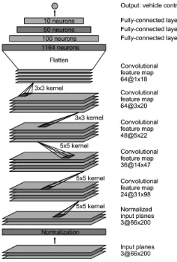
One of these wonders that has always fed the imagination and dreams of many people is the autonomous car. In the 80’s TV series like Knight Rider have predicted the possibilities in the near future of such technologies. Nowadays, technology newspapers and blogs are filled by article about how it works but they never go in much detail. The main reason is that car manufactures have always avoided to disclose their secrets. Nevertheless, research papers such as [1] or [2] have paved the way for disseminating these technoglogies, for example by showing successful applications or artificial neural networks in tasks such as traﬃc sign recognition or lane keeping driver assistant. In particular, the work in [2] exploits deep learning methods, such as Convolutional Neural Networks in order to teach a car to steer and drive using supervised learning with a wide dataset. Deep Learning can be summed up as a sub field of Machine Learning studying statical models called deep neural networks. The latter are able to learn complex and hierarchical representations from raw data, unlike hand crafted models which are made of an essential features engineering step. Especially during the last five

(8)

classification, objects detection, object localization, object tracking, pose estimation, image segmentation or image captioning.

Among the various paradigms in machine learning, a prominent one is reinforcement learning, which has recently attracted the attention of scholars and developers and has proven to lead to outstanding results.

Reinforcement learning is a known field in cognitive science that focuses on the study of thinking processes. The main idea is that learning happens with the help of a feedback coming from the outer world as a response to an action. In psychology, the idea of trial-and-error has been expressed by Edward Thorndike in 1911 [3]. So, this very idea existed for a long time until it could become the basis of a machine learning paradigm. In fact, the idea of applying these concepts to computers is not new, as it was already proposed when the notion of computational machine was proposed by Turing [3]. In its early stages, it was first combined with supervised learning, and took its own way in 70s, when the method was formalized and improved.

Lately, DeepMind (former Google Brain Team) made important contri-butions in artificial intelligence by using reinforcement learning algorithms together with deep learning techniques in neural networks. They have pub-lished some state-of-the-art papers that became milestone for the current technological advancements. These include the papers Playing Atari with Deep Reinforcement Learning [4] - 2013, where deep Q-learning is used, and the biggest most recent breakthrough, Mastering the Game of Go with Deep Neural Networks and Tree Search [5] - 2016, where reinforcement learning Monte Carlo tree search is used with Q-learning. Also, in June 2016, they published a paper Asynchronous Methods for Deep Reinforcement Learning [6] that provides a clear comparison of the diﬀerent deep reinforcement learn-ing algorithms for the asynchronous trainlearn-ing and introduces an algorithm - Asynchronous Advantage Actor-Critic that surpasses the performances of

(9)

Introduction iii

In this abundant flow of discoveries in artificial intelligence and deep rein-forcement learning, the reuse of new techniques and their further exploration needs to be investigated and studied in more detail. The goal of this work is to dive in this world and show in a specific use case which one behave the best. The specific use case consists of a company which need to start from scratch and want to develop its own ADAS (Advanced Driver Assistance Systems) with no dependence from any of the vendors which provide camera or sensors. The main objective of this work is to study and analyse the most relevant techniques in deep learning and compare them in the case of autonomous driving. The context of this work is an industrial environment in which a company wants to develop its own Advanced Driver Assistance System with total independence form vendors providing cameras and sensors.

Chapter 1 provides the theoretical background on autonomous driving, machine learning and computer vision.

Chapter 2 illustrates methods, algorithms and neural networks architec-tures that are best suited for autonomous driving.

Chapter 3 describes all the choices that have been made behind the development of the algorithms. Comparison are shown among programming languages, GPU and CPU, Simulators and Deep Learning Frameworks

All the algorithms and techniques developed in this thesis are described in detail in Chapter 4, while in Chapter 5 experimental results are shown.

Finally, the last chapter summarizes the work done and provides an outlook to future developments.

(10)

(11)

List of Figures

1.1 1960 British self-driving car . . . 3

1.2 ARGO internal and external equipment . . . 4

1.3 Google Driverless Car . . . 5

1.4 A Self-Driven 2008 Toyota by Google . . . 6

1.5 Vislab Autonomous Vans . . . 7

1.6 SAE Classification . . . 9

1.7 Prediction steps for all cars fully autonomous . . . 10

1.8 Feed-forward ANN . . . 17

1.9 CNN arranges its neuron in 3 dimensions . . . 19

1.10 Example of a CNN input volume . . . 21

1.11 Spatial arrangement example . . . 22

1.12 Linear vs. Recurrent unit . . . 24

1.13 LSTM functionality . . . 26

1.14 Agent - Environment interaction. . . 30

1.15 The backup diagrams for v⇤ and q⇤ . . . 33

2.1 Three paradigms for autonomous driving. . . 39

2.2 ALVINN architecture and NAVLAB . . . 41

2.3 Birds Eye View Transform and transformation to obtain the line 43 2.5 NVIDIA model . . . 47

2.6 Deep Learning for Self-Driving Car summary. . . 49

2.7 Deep RL architectures. . . 50

3.1 GitHub followers comparison . . . 67 ix

(16)

3.2 Diﬀerences between CPU and GPU . . . 70

3.3 Python version of DeepTesla screen-shot . . . 72

3.4 Udacity Simulator screen-shot . . . 73

3.5 Screenshots from the TORCS environment . . . 74

3.6 Three of the fourteen diﬀerent weather condition oﬀered by CARLA Simulator. . . 75

4.1 DeepTesla data distribution . . . 81

4.3 CARLA training data distribution . . . 83

4.4 Chessboard calibration. . . 84

4.5 Chessboard calibration. . . 84

4.6 Threshold binary transformation examples . . . 86

4.7 Bird’s Eye View. . . 87

4.8 Polyfit functions results . . . 88

4.9 A general comparison using MNIST between diﬀerent optimizer using the same Neural Network. Image taken from [7] . . . 93

4.10 Model CNN for DeepTesla implementation . . . 96

4.11 CNN model for DeepTesla implementation . . . 98

4.14 The ANN structure of the A3C implementation into CARLA . 105 4.15 A3C Flow . . . 106

4.12 Model CNN LSTM for DeepTesla implementation . . . 109

4.13 CNN model for CARLA implementation . . . 110

5.1 Results obtained during the evaluation of Traditional Image Processing solution using DeepTesla. . . 112

5.2 Results obtained while testing CNN solution for DeepTesla. . . 113

5.3 Results obtained while testing CNN LSTM solution for DeepTesla.113 5.4 Training(up) and validation(down) losses . . . 115

5.5 Four agents working in diﬀerent conditions . . . 116

5.7 Example of semantic segmentation . . . 121

5.8 Representation of the environment reconstruction using LiDAR technology . . . 122

(17)

Chapter 1 Theoretical Background

In this chapter, an overview of the main concepts at the background of this work is provided and the related technologies that will be dealt with in the following chapters are described. In particular, the work is focused on:

1. Self Driving Car (SDC): it is an Unmanned Ground Vehicle capable of sensing its environment and navigating without human input. 2. Machine Learning (ML): Machine Learning is a method of data

analysis that automates analytical model building. It is a branch of artificial intelligence based on the idea that machines should be able to learn and adapt through experience [8]. In those section I will also describe Deep Learning (DL) and I will introduce Artificial Neural Networks (ANNs)

3. Convolutional Neural Networks (CNNs): it is a class of deep, feed-forward ANNs that has successfully been applied to analysing visual imagery. Although they belong to Computer Vision field, I will treat it on a separate section for the relevance they will have in this work. 4. Recurrent Neural Networks (RNNs): class of ANNs where

connec-tions between units form a directed cycle. This property allows them to exhibit dynamic temporal behaviour.

(18)

5. Reinforcement Learning (RL): area of ML inspired by behaviourist psychology, concerned with how software agents ought to take actions in an environment so as to maximize some notion of cumulative reward. 6. Computer Vision (CV): discipline that deals with how computers

can be made for gaining high-level understanding from digital images or videos.

In the following sections of this chapter, the above mentioned subjects will be described with the aim of providing a background to the modelling, designing and development a Self-Driving Car.

1.1 Self-Driving Car

A Self-Driving Car (SDC) or autonomous car is an Unmanned Ground Vehicle that is a vehicle capable of sensing its environment and navigating without human input [9].

Autonomous cars use many sensors which are able to perceive the sur-rounding environment. Sensors used could be radars, laser lights, GPS sensors or vision sensors. Advanced control systems interpret sensory information to plan appropriate navigation paths, as well as to recognise obstacles and relevant traﬃc signals.[10, 11] Autonomous cars must have control systems that are capable of analysing sensory data to distinguish between diﬀerent cars on the road.

Many such systems are evolving, but by now no cars permitted on public roads were fully autonomous. They all require a human at the wheel who must be ready to take control at any time.

1.1.1 History and the State of the Art

The first examples of Self-Driving Car has to be found in 1920s were Houdina Radio Control demonstrated the radio-controlled American Wonder on New York City streets. In 1957, a full size system was successfully

(19)

1.1 Self-Driving Car 3

Figure 1.1: 1960 British self-driving car that interacted with magnetic cables that were embedded in the road. It went through a test track at 80 miles per hour (130 km/h) without deviation of speed or direction in any weather conditions, and in a far more eﬀective way than by human control [12, 13, 14]. Image taken from [13]

demonstrated by RCA Labs and the State of Nebraska on a 400-foot strip of public highway at the intersection of U.S. Route 77 and Nebraska Highway 2, then just outside Lincoln, Nebraska. A series of experimental detector circuits buried in the pavement were a series of lights along the edge of the road. The detector circuits were able to send impulses to guide the car and determine the presence and velocity of any metallic vehicle on its surface[18, 19]. During the years, many examples of autonomous cars were revealed by research laboratories, but more relevant project has been created in the 1990s[12, 13, 14, 20, 21, 22].

In 1995, Carnegie Mellon University’s Navlab project completed a 3,100 miles (5,000 km) cross-country journey, of which 98.2% was autonomously controlled, dubbed No Hands Across America. This car, however, was semi-autonomous by nature: it used neural networks to control the steering wheel, but throttle and brakes were human-controlled, chiefly for safety reasons.[21, 22]

(20)

Figure 1.2: ARGO’s equipment from an external(a) and internal perspective(b). Image taken from [15]

Project, which worked on enabling a modified Lancia Thema (see Figure 1.2) to follow the normal (painted) lane marks in an unmodified highway[23, 15].The culmination of the project was a journey of 1,200 miles (1,900 km) over six days on the motorways of northern Italy dubbed Mille Miglia in Automatico ("One thousand automatic miles"), with an average speed of 56 miles per hour (90 km/h)[24]. The car operated in fully automatic mode for 94% of its journey, with the longest automatic stretch being 34 miles (55 km). The vehicle had only two black-and-white low-cost video cameras on board and used stereoscopic vision algorithms to understand its environment.

In 2004, DARPA (the Defense Advanced Research Projects Agency) launched the first Grand Challenge event and oﬀered a $1 million prize to any team of engineers which could create an autonomous car able to finish a 150-mile course in the Mojave Desert. No team was successful in completing the course[25]. In October 2005, the second DARPA Grand Challenge was again held in a desert environment. GPS points were placed and obstacle types were located in advance [26]. In this challenge, five vehicles completed the course. In November 2007, DARPA again sponsored Grand Challenge III, but this time the Challenge was held in an urban environment. In this race, a 2007 Chevy Tahoe autonomous car from Carnegie Mellon University earned

(21)

Figure 1.3: Google Driverless Car. Image taken from Grendelkhan,2016

the 1st place. Prize competitions as DARPA Grand Challenges gave students and researchers an opportunity to research a project on autonomous cars to reduce the burden of transportation problems such as traﬃc congestion and traﬃc accidents that increasingly exist on many urban residents[26].

Many major automotive manufacturers, including General Motors, Ford, Mercedes Benz, Volkswagen, Audi, Nissan, Toyota, BMW, and Volvo, are testing driverless car systems as of 2013. BMW has been testing driverless systems since around 2005,[27, 28] while in 2010, Audi sent a driverless Audi TTS to the top of Pike’s Peak at close to race speeds.[29] In 2011, GM created the EN-V (short for Electric Networked Vehicle), an autonomous electric urban vehicle[30].

In 2010, Italy’s VisLab from the University of Parma, led by Professor Al-berto Broggi, ran the VisLab Intercontinental Autonomous Challenge (VIAC), a 9,900-mile (15,900 km) test run which marked the first intercontinental land journey completed by autonomous vehicles. Four electric vans made a 100-day journey, leaving Parma on 20 July 2010, and arriving at the Shanghai Expo in China on 28 October. Although the vans were driverless and mapless, they did carry researchers as passengers in case of emergencies. The experimenters did have to intervene a few times - when the vehicles got caught in a Moscow traﬃc jam and to handle toll booths[17].

(22)

Figure 1.4: In Las Vegas, Chris Urmson, now head of Google’s self-driving car project, tested a 2008 Toyota autonomously driven and was in the driver seat in case anything went wrong. Google had previously mapped the area and selected a route for the test, which the DMV agreed to. Image taken from [16]

On May 1, 2012, a 22 km (14 mi) driving test was administered to a Google self-driving car by Nevada motor vehicle examiners in a test route in the city of Las Vegas, Nevada. The autonomous car passed the test, but was not tested at roundabouts, no-signal rail road crossings, or school zones.[16] In 2013, on July 12, VisLab conducted another pioneering test of au-tonomous vehicles, during which a robotic vehicle drove in down town Parma with no human control, successfully navigating roundabouts, traﬃc lights, pedestrian crossings and other common hazards[31].

Although as of 2013, fully autonomous vehicles are not yet available to the public, many contemporary car models have features oﬀering limited autonomous functionality. These include adaptive cruise control, a system that monitors distances to adjacent vehicles in the same lane, adjusting the speed with the flow of traﬃc; lane assist, which monitors the vehicle’s position in the lane, and either warns the driver when the vehicle is leaving its lane, or, less commonly, takes corrective actions; and parking assist, which assists the driver in the task of parallel parking[32].

In October 2014, Tesla Motors announced its first version of AutoPilot. Model S cars equipped with this system are capable of lane control with

(23)

Figure 1.5: Driverless electric vans complete 8,000 mile journey from Italy to China. Image taken from [17]

autonomous steering, braking and speed limit adjustment based on signals image recognition. The system also provide autonomous parking and is able to receive software updates to improve skills over time[33]As of March 2015, Tesla has been testing the autopilot system on the highway between San Francisco and Seattle with a driver but letting the car to drive the car almost unassisted.[34]

Tesla Model S Autopilot system is suitable only on limited-access highways not for urban driving. Among other limitations, Autopilot can not detect pedestrians or cyclists[35]. In March 2015 Tesla Motors announced that it will introduce its Autopilot technology by mid 2015 through a software update for the cars equipped with the systems that allow autonomous driving[34]. Some industry experts have raised questions about the legal status of autonomous driving in the U.S. and whether Model S owner would violate current state regulations when using the autopilot function. The few states that have passed laws allowing autonomous cars on the road limit their use for testing purposes, not the use by the general public. Also, there are questions about the liability for autonomous cars in case there is a mistake[34].

In February 2015 Volvo Cars announced its plans to lease 100 XC90 SUVs fitted with Drive Me Level 3 automation technology to residents of Gothenburg in 2017[36, 37]. The Drive Me XC90s will be equipped with

(24)

NVIDIA’s Drive PX 2 supercomputer, and will be driven autonomously in certain weather conditions and on one road that loops around the city[38].

In July 2015, Google announced that the test vehicles in its driverless car project had been involved in 14 minor accidents since the project’s inception in 2009. Chris Urmson, the project leader, said that all of the accidents were caused by humans driving other cars, and that 11 of the mishaps were rear-end collisions. Over the six years of the project’s existence the test vehicles had logged nearly 2 million miles on the road[39, 25].

The first known fatal accident involving a vehicle being driven by itself took place in Williston, Florida on 7 May 2016 while a Tesla Model S electric car was engaged in Autopilot mode. The driver was killed in a crash with a large 18-wheel tractor-trailer. On 28 June 2016 the National Highway Traﬃc Safety Administration (NHTSA) opened a formal investigation into the accident working with the Florida Highway Patrol. According to the NHTSA, preliminary reports indicate the crash occurred when the tractor-trailer made a left turn in front of the Tesla at an intersection on a non-controlled access highway, and the car failed to apply the brakes. The car continued to travel after passing under the truck’s trailer.[40, 41] The NHTSA’s preliminary evaluation was opened to examine the design and performance of any automated driving systems in use at the time of the crash, which involves a population of an estimated 25,000 Model S cars[42]. In August 2016 Singapore launched the first self-driving taxi service, provided by nuTonomy[43].

1.1.2 Autonomous instead of automated

Autonomy generally means freedom from external control. Usually, when an agent, or a vehicle or a robot is said to be autonomous, it is meant to be with a certain degree of autonomy because an agent could have dependence from environment or other agents in many diﬀerent ways. It is not an all-or-nothing issue, but a matter of degree [45]. Because of this reason, autonomous driving has been classified using a system based on six diﬀerent levels (ranging from

(25)

Figure 1.6: SAE Classification. Image taken from [44]

fully manual to fully automated systems) that was published in 2014 by SAE International, an automotive standardization body, as J3016, Taxonomy and Definitions for Terms Related to On-Road Motor Vehicle Automated Driving Systems.[44] This classification system is based on the amount of driver intervention and attentiveness required, rather than the vehicle capabilities, although these are very loosely related.

These levels are very important because they help to identify the real nature of the vehicle. Actually, there is no commercial Level 4/ Level 5 vehicle on the road, but only some level 3. For example, in 2017 Audi stated that its latest A8 would be autonomous using its Audi AI. Billed by Audi as the traﬃc jam pilot it takes charge of driving in slow-moving traﬃc at up to 60 km/h on motorways where a physical barrier separates the two carriageways. The driver would not have to do safety checks such as frequently gripping the steering wheel. The Audi A8 was claimed to be the first production car to reach level 3 autonomous driving and Audi would be the first manufacturer to use laser scanners in addition to cameras and ultrasonic sensors for their system.[46]

1.1.3 Advantages

Autonomous driving has not a long history since the first real approaches but it may introduce several advantages once deployed for commercial purpose.

(26)

Figure 1.7: Prediction that show the steps that it will be taken to have all cars fully autonomous . Image taken from [47]

• Safety: autonomous driving should reduce to a minimum the risk of an accidental error caused by human distraction or aggressive driving. For human error it is meant rubbernecking, delayed reaction time, tailgating, and other forms of distracted or aggressive driving [47, 48, 49].

• Welfare: Autonomous cars could relieve travellers from driving and navigation chores, thereby replacing behind-the-wheel commuting hours with more time for leisure or work;[47, 50] and also would lift constraints on occupant ability to drive, distracted and writing SMS while driving, intoxicated, prone to seizures, or otherwise impaired.[51, 25]. For the young, the elderly, people with disabilities, and low-income citizens, autonomous cars could provide enhanced mobility.[52, 53, 54]

• Traﬃc: Advantages that comes from autonomous driving cars could also include higher speed limits;[55] smoother rides;[56], increased roadway capacity and minimized traﬃc congestion, due to decreased need for

(27)

safety gaps and higher speeds[57]. Currently, maximum controlled-access highway throughput or capacity according to the U.S. Highway Capacity Manual is about 2,200 passenger vehicles per hour per lane, with about 5% of the available road space is taken up by cars. It has been estimated that autonomous cars could increase capacity by 273% ( 8,200 cars per hour per lane)[58].

• Costs: Safer driving could reduce the costs of vehicle insurance[59, 58]. Reduced traffic congestion and the improvements in traffic flow due to widespread use of autonomous cars will also translate into better fuel efficiency. [53, 60]

1.1.4 Obstacles

In spite of the benefits related to increased vehicle automation, there are many foreseeable challenge which persist. For example, there are disputes concerning liability, the time needed to turn the existing stock of vehicles from non-autonomous to autonomous,[61] resistance by individuals to forfeit control of their cars,[62] customer concern about the safety of driverless cars,[63] and the implementation of legal framework and establishment of government regulations for self-driving cars.[64]. Other obstacles could be missing driver experience in potentially dangerous situations[65], ethical problems in situations where an autonomous car’s software is forced during an unavoidable crash to choose between multiple harmful courses of action[66, 67, 68], and possibly insuﬃcient Adaptation to Gestures and non-verbal cues by police and pedestrians[69].

Possible technological obstacles for autonomous cars are: • Software reliability.[70]

• A car’s computer could potentially be compromised, as could a commu-nication system between cars[71, 72, 73, 74, 75].

(28)

types of weather or deliberate interference, including jamming and spoofing[69].

• Avoidance of large animals requires recognition and tracking, and Volvo found that software suited to caribou, deer, and elk was ineﬀective with kangaroos[76].

• Autonomous cars may require very high-quality specialised maps[77] to operate properly. Where these maps may be out of date, they would need to be able to fall back to reasonable behaviours[69, 78].

• Field programmability for the systems will require careful evaluation of product development and the component supply chain.[75]

• Current road infrastructure may need changes for autonomous cars to function optimally [79]

• Cost (purchase, maintenance, repair and insurance) of autonomous vehi-cle as well as total cost of infrastructure spending to enable autonomous vehicles and the cost sharing model.

• A direct impact of widespread adoption of autonomous vehicles is the loss of driving-related jobs in the road transport industry[59, 80]. There could be job losses in public transit services and crash repair shops. The car insurance industry might suﬀer as the technology makes certain aspects of these occupations obsolete[53].

• Research shows that drivers in autonomous cars react later when they have to intervene in a critical situation, compared to if they were driving manually[81].

1.2 Machine Learning

There are problems that could be considered very diﬃcult to be formulated and it happens that is extremely diﬃcult to write programs that can solve

(29)

1.2 Machine Learning 13

some type of problems satisfactorily. Sometimes the solution found may be hard to be understood and so they lack of generality. Such algorithm could not be so robust to work when noisy data are used and so they may introduce maintenance problems. A viable solution to this kind of problems is machine learning. Generally speaking, a machine learning problem consists of lots of data to be considered in order to obtain an eﬃcient and robust behaviour by the program. Data are fundamental in such kind of programs because they influence learning. Lots of data and correct data are essential part of machine learning algorithm. In fact, such algorithm takes these examples and produces a program that does the job. Usually there may be some task that will require to evaluate data which it has never been considered. A machine learning algorithm is said to be robust if it correctly evaluates also these data. Moreover, machine learning algorithm could provide mechanisms that make the program change on-the-job. This feature when related to human is called learning by experience. An important definition was given by Mitchell who said that A computer program is said to learn from experience E with respect to some class of tasks T and performance measure P , if its performance at tasks in T , as measured by P , improves with experience E[82]. Such definition is relevant because gives a general overview of what is the intrinsic relation between experience and learning. Machine learning tasks are typically classified into three broad categories, depending on the nature of the learning signal or feedback available to a learning system[83]. These are: • supervised learning: paradigm that uses sets of data already collected in order to provide input-output relationships. Those data provides feedback to the learning process and, as long as it computes, it has to derive a model also for unknown relationship. Usually algorithms that follow such paradigm are able to solve classification problem (a.k.a. pattern recognition) and regression problem.

• unsupervised learning: paradigm that has input data which do not have target outputs given. It has to learn how data are organised, discover patterns or build a representation of them. Usually algorithms that

(30)

follow such paradigm are able to solve clustering type problems. • reinforcement learning: paradigm which addresses the question of how

an autonomous agent that senses and acts in its environment can learn to choose optimal actions to achieve its goal. Usually, input data are generated by the agent’s interaction with the environment. A critic provides a reward or a penalty to indicate the desirability of the resulting behaviour. The evaluation from the critic represents the feedback to be used in the learning process. The task of the agent is to learn from this indirect, delayed reward, to choose sequences of actions that produce the greatest cumulative reward.

Machine learning grew out of the quest for AI. Already in the early days of AI as an academic discipline, some researchers were interested in having machines that learn from data. They attempted to approach the problem with various symbolic methods, as well as what were then termed "neural networks"; these were mostly perceptrons and other models that were later found to be reinventions of the generalized linear models of statistics[84].

1.2.1 Deep Learning

During 1980s, machine learning algorithm like Support vector machines and other, much simpler methods such as linear classifiers gradually overtook neural networks in machine learning popularity. Earlier challenges in training deep neural networks were successfully addressed with methods such as un-supervised pre-training, while available computing power increased through the use of GPUs and distributed computing. Neural networks were deployed on a large scale, particularly in image and visual recognition problems. This became known as deep learning, although deep learning is not strictly synony-mous with deep neural networks. Deep learning is a class of machine learning algorithms that:

• "use a cascade of many layers of non-linear processing units for feature extraction and transformation. Each successive layer uses the output

(31)

from the previous layer as input. The algorithms may be supervised or unsupervised and applications include pattern analysis (unsupervised) and classification (supervised)"(quoted from [85]).

• "are based on the (unsupervised) learning of multiple levels of features or representations of the data. Higher level features are derived from lower level features to form a hierarchical representation.

• "are part of the broader machine learning field of learning representations of data"(quoted from [85]).

• "learn multiple levels of representations that correspond to diﬀerent levels of abstraction; the levels form a hierarchy of concepts.

• "use some form of gradient descent for training via back-propagation" (quoted from [85])

"These definitions have in common multiple layers of non-linear processing units and the supervised or unsupervised learning of feature representations in each layer, with the layers forming a hierarchy from low-level to high-level features"(quoted from [85]). The composition of a layer of non-linear processing units used in a deep learning algorithm depends on the problem to be solved. Layers that have been used in deep learning include hidden layers of an artificial neural network and sets of complicated propositional formulas[86]. They may also include latent variables organized layer-wise in deep generative models such as the nodes in Deep Belief Networks and Deep Boltzmann Machines[87].

The assumption underlying distributed representations is that observed data are generated by the interactions of layered factors. Varying numbers of layers and layer sizes can provide diﬀerent amounts of abstraction[88]. Deep learning exploits this idea of hierarchical explanatory factors where higher level concepts are learned from the lower level ones [89, 90]. Deep learning helps to disentangle these abstractions and pick out which features are useful for improving performance[88]. For supervised learning tasks, deep

(32)

learning methods obviate feature engineering, by translating the data into compact intermediate representations similar to principal components, and derive layered structures that remove redundancy in representation.[91, 85] Deep learning algorithms can also be applied to unsupervised learning tasks. This is an important benefit because unlabelled data are more abundant than labelled data. Examples of deep structures that can be trained in an unsupervised manner are neural history compressors[91, 92] and deep belief networks[88, 87].

1.2.2 Artificial Neural Networks

ANNs are computing systems inspired by the biological neural networks that constitute brains. Their properties and functionality have been success-fully replicated in ANNs. An ANN is a layered structure of neurons which has minimum one input layer and one output layer. Each layer has a number of units (neurons) that are connected to the units in another layer. The connections are assigned weights that are used for the unit’s activation. In order to perform activation, a weighted sum of its inputs is computed at each unit and then passed to an activation function to produce output. There are diﬀerent activation functions, though, and the choice depends on the type of problem.

Depending on the structure of the network, there are diﬀerent types of ANNs. For example, a simple case of feed-forward ANN without any loops, with an input layer of 4 units, 2 hidden layers, and an output layer with 2 units is presented in the Figure 1.8:

(33)

Figure 1.8: Feed-forward ANN

Some ANNs can be proclaimed as deep. This qualifier describes the networks that have many hidden layers, precisely more than two. More hidden layers would compute more abstract representations of the input data, which means richer features. Deep ANNs are harder to train, but they are more powerful and are especially used in modern artificial intelligence applications.

Usually, ANNs learn by an SGD method. More precisely, learning implies the definition of an objective function that describes the performance of the network, and, which is either minimized or maximized. An objective function can be the loss of the network over a set of training examples. In RL, an ANN can use TD errors in computing the loss function and learning the value function, or maximize the reward, or use a policy gradient algorithm [3]. No matter the case, the partial derivatives are required to determine the influence of a weight change on the network’s performance, and they can be obtained with the help of the gradient.

In order to find the gradient, an ANN can use the back-propagation algorithm. In the forward pass, the network’s units would compute the outputs, whereas in the backward pass - the partial derivatives with respect to each weight. However, the back-propagation algorithm isn’t that eﬃcient for the deep ANNs, because of the overfitting problem.

(34)

Deep Neural Networks

A special structure of the network’s architecture, like that of the deep con-volutional networks (CNN) would make it possible to use the back-propagation algorithm in deep ANNs, too. CNN is a very important type of ANN that is especially used for finding spatially correlated patterns in images while sharing weights and excluding the need of full connectivity between units. A deep neural network (DNN) is an ANNs with multiple hidden layers between the input and output layers[86, 92]. Similar to shallow ANNs, DNNs can model complex non-linear relationships. DNN architectures generate com-positional models where the object is expressed as a layered composition of primitives[93]. The extra layers enable composition of features from lower layers, potentially modelling complex data with fewer units than a similarly performing shallow network.[86]

1.3 Convolutional Neural Networks (CNNs)

Convolutional Neural Networks are similar to normal neural networks. They are made up of neurons that can learn weights and biases. Each neuron receives some input, performs a dot product, and, sometimes, follows with a non-linearity function. The whole network expresses a single diﬀerentiable score function - from raw image pixels to class scores. CNN architectures assume that the inputs are images, which make it possible to encode certain properties into the architecture. It makes the forward function more eﬃcient to implement, and it reduces the number of parameters in the network. [94] The problem about regular neural networks is that it doesn’t scale well to full images. An example is the CIFAR-10 [95], where the images are only of the size 32 ⇥ 32 ⇥ 3 (32 wide, 32 high, 3 colour channels). A single fully-connected neuron in the first hidden layer of a regular Neural Network would have 32 · 32 · 3 = 3072 weights. For bigger sizes images, e.g. 200 ⇥ 200 ⇥ 3, it would lead to neurons that have 200 · 200 · 3 = 120000 weights. This full connectivity is wasteful and the huge number of parameters would quickly

(35)

1.3 Convolutional Neural Networks (CNNs) 19

lead to overfitting. Convolutional neural networks take advantage of the fact that the input consists of images. The layers of a CNN have neurons arranged in 3 dimensions: width, height, depth. In the example of the CIFAR-10 [95] the input is a volume of activations, and the volume has the dimensions 32x32x3 (width, height, depth respectively). The neurons in a layer will only be connected to a small region of the previous layer, unlike the fully connected manner in regular NN. In order to visualize this diﬀerence, the Figure 1.8 with the feed-forward structure of an ANN can be compared as in the Figure Figure 1.9.

Figure 1.9: A Convolutional Neural Network arranges its neurons in three dimensions (width, height, depth), as visualized in one of the layers. Every layer of a CNN transforms the 3D input volume to a 3D output volume of neuron activations. In this example, the red input layer holds the image, so its width and height would be the dimensions of the image, and the depth would be 3 (Red, Green, Blue channels). Image taken from [94]

.

1.3.1 Layers

As described earlier a CNN is a combination of layers and every layer transforms one volume of activations into another through a diﬀerentiable function. CNN uses three main types of layers to build the architecture: Convolutional Layer, Pooling Layer, and Fully-Connected Layer (exactly as seen in regular Neural Networks on Figure 1.8). These layers will be stacked to form a full CNN architecture. In reinforcement learning the pooling layer is not used because they buy translation invariance - the network becomes insensitive to the location of an object in the image.

(36)

Convolutional Layer

The Convolutional layer is the main building block of a convolutional neural network. It does most of the computational heavy lifting. The convolutional layer consists of filters which learn. Every filter is spatially small (along width and height), but extends to the full depth of the input volume. An example of the first layer in a CNN is a filter with the size 5 ⇥ 5 ⇥ 3. During the first forward pass, the data is slide/convolved through each filter across the height and width of the input volume, and the dot products between the entries of the filter and the input at any position are computed. As the filter slides over the input volume it produces a 2-dimensional activation map. The activation map shows the responses of that filter at all spatial positions. The network will learn filters that activate when they see some type of visual features - such as an edge of some orientation or a patch of some colours. On higher layers the network will learn to see more complex patterns: it could be honeycomb or wheel-like patterns. On each convolutional layer, there will be an entire set of filters, each layer will produce a separate 2-dimensional activation map. The activation maps will be stacked along the depth dimension and produce the output volume. When dealing with high dimensional inputs like images, it is impractical to connect neurons to all the neurons in the previous volume. A smarter solution is to connect each neuron to only a local region of the input volume instead. The spatial extent of this connectivity is a hyperparameter called the receptive field of the neuron - equivalently this is the filter size. An illustration of the receptive field can be seen on 1.10.

Spatial arrangement

The connectivity of each neuron in the convolutional layer to the input volume is described by the spatial arrangement. Spatial arrangement describes how many neurons there are in the output volume and how they are arranged. Three hyperparameters control the size of the output volume - depth, stride, and zero-padding.

(37)

1.3 Convolutional Neural Networks (CNNs) 21

Figure 1.10: An example input volume in red (e.g. a 32x32x3 CIFAR-10 image), and an example volume of neurons in the first Convolutional layer in blue. Each neuron in the convolutional layer is connected only to a local region in the input volume spatially, but to the full depth (i.e. all colour channels). Note, there are multiple neurons (5 in this example) along the depth, all looking at the same region in the input. Image taken from [94]

the convolutional layer uses. Each filter looks for something diﬀerent in the input. For example, the convolutional layer takes a raw image as an input, then the diﬀerent neurons along the depth dimension may activate in the presence of various oriented edges or blobs of colours. A set of neurons that look at the same region of the input is called depth column or fibre.

Another hyperparameter is the stride. It defines how the filters slide over the input. If the stride is 1, then the filters move one pixel at a time. When the stride is 2, then the filters move 2 pixels at a time. This will produce spatially smaller output volumes.

The last hyperparameter to control the size of the output volume is the size of zero-padding. Zero-padding pads the input volume with zeros around the border. The good feature of zero-padding is that it controls the spatial size of the output volumes. This is useful to preserve the spatial size of the input volume so that the input and output width and height are the same.

The way to compute the spatial size of the output volume is by using a function of the input volume size (W), the receptive field size of the

(38)

convolutional layer neurons (F), the stride with which they are applied (S), and the amount of zero padding used (P) on the border. The formula for calculating how many neurons "fit" is the following:

W F + 2P

S + 1 (1.1)

An example for a 5x5 input and a 3x3 filter with stride 1 and zero-padding 1 the output would be of the spatial size 5x5:

5 3 + 2· 1

1 + 1 ! 4

1 + 1 = 5 (1.2) And with stride 2 the output would be 3x3:

7 3 + 2_{· 1}

2 + 1 ! 4

2 + 1 = 3 (1.3) The visualization is provided on the figure below Figure 1.11:

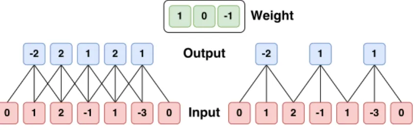
Figure 1.11: Illustration of spatial arrangement. The example is described above. In this example, there is only one spatial dimension (x-axis), one neuron with a receptive field size of F = 3, the input size is W = 5, and there is zero-padding of P = 1. Left: The neuron strides across the input in stride of S = 1. Right: The neuron uses stride of S = 2. The neuron weights are in this example [1,0,-1] (shown on very right), and its bias is zero. These weights are shared across all yellow neurons. Image taken from [94].

1.3.2 Fully connected Layer

The fully connected layer in CNNs is a traditional Multi-Layer Perceptron. The term “Fully Connected” implies that every neuron in the previous layer is connected to every neuron in the next layer as seen on Figure 1.8. The

(39)

1.4 Recurrent Neural Networks (RNNs) 23

output from the convolutional layers represents a high-level feature of the input image. The purpose of the Fully Connected layer is to use these features for classifying the input images into various classes.

Apart from classification, the fully connected layer is also a cheap way to learn non-linear features. By combining these features, the classification of the network would be even better [96].

1.4 Recurrent Neural Networks (RNNs)

Recurrent neural networks (RNN) are used when the patterns in data change with time. RNNs have a simple structure with a built-in feedback loop allowing it to act as a forecasting engine. RNNs are applied in a large range of applications, from speech recognition to driver-less cars.

In feed-forward neural networks the data flows in one direction only, whereas in RNN the output of the layer is added to the input of the same layer, and this layer represents the whole network. This results in a loop-like network. The flow can be viewed or interpreted as a time passage where at each time-step the same layer receives it’s own output from the previous time-step and adds it up to the input part together with the new data received [97].

Unlike feed-forward ANNs, RNNs can work with sequences of data inputs and, subsequently, to output sequences of data in return. Not only RNNs use sequence of data but also these sequences can vary in their size, so diﬀerent sizes of sequences can be adapted by the RNN dynamically. Another key feature of the RNN is the dependency of the training examples. Unlike feed-forward ANNs, where the training examples are independent of each other, the RNNs treat temporal dependencies, meaning that a sequence of e.g. words is usually dependent on what came before [98]. These new features open a new range of applications like image captioning (single input, sequence output), document classification (sequence input, single output), video frames classification (sequence input, sequence output), demand and supply chain

(40)

planning forecasting (with added time delay) [97].

In order to understand better the recurrent neuron functionality, the Figure 1.12 presents a comparison between the RNN unit and the linear unit used in feed-forward ANNs.

Figure 1.12: Linear vs. Recurrent unit

A linear unit’s output is the input xj times the weight matrix Wij which

is then passed to an activation function g.

yi = g(

X

j

Wijxj+ b) (1.4)

The recurrent unit is composed of a linear unit, but then it adds a recurrent weight WR, therefore the output h(t) depends on both the input xt and the

activity at the previous time-step. To retrieve an output yt from the layer, a

non linear activation function gy is applied to the h(t) [98].

h(t) = gh(WIx(t)+ WRh(t 1)+ bh)

y(t) = gy(Wyh(t)+ by)

(1.5)

For example, in case of word prediction, the input of a unit can be a word, and the output of that unit would be the predicted next word that follows the one that was input; then, when the next input comes in at the next time-step, the process is applied, but also with the activity at the previous time-step taken into account.

The training of RNNs is diﬀerent than that of the other ANNs, because RNNs emit an output at each time-step, and, therefore, there is a cost

(41)

1.4 Recurrent Neural Networks (RNNs) 25

function at each time-step, whereas before, in feed-forward networks, it was necessary to run the input through the whole network in order to get an output comparable to the one and only cost function. Another special characteristic of the RNNs is that the weights WR are shared across the network. So, the

gradients from all the time-steps can be combined together to obtain the weights update and do back-propagation. But, because of the shared weights, the update would scale with the size of the WR, the back-propagation has

to be done all the way until time-step zero, which causes the problem of vanishing and exploding gradients [98].

1.4.1 Gating in RNN

In order to address the problems of training deep RNNs, there are diﬀerent solutions available. Among the known solutions are the use of the Root Mean Square Propagation (RMSProp) optimizer for learning rate adjustment, clipping gradients, ReLu activation functions, special weight initialization, or to use gating [98]. Gating is a technique for deciding when to forget the current input, and when to remember it for future time steps [97]. The most famous approaches are long short-term memory (LSTM) and gated recurrent units (GRU).

LSTM has at its core a memory cell C with a recurrent weight WC = 1

that inherits the activity of the previous time-step. This memory cell has three manipulations: forget (flush the memory), input (add to the memory), and output (retrieve from the memory) [98]. The activity of the memory cell Ct is taken and passed through a tanh activation function and multiplied

by the gate. The gate is an aﬃne layer, or a ’standard’ feed-forward ANN layer, that has as inputs xt at the current time-step and ht 1 of the previous

time-step that are together multiplied by the weight W0, summed and passed

through the sigmoid activation function to return a vector of numbers between 0 and 1. The gate operation for generating the output ht, or for

getting the information from the memory cell Ct, is presented in the following

(42)

ht= (W0· [xtht 1] + b0) tanh(Ct)

= ot tanh(Ct)

(1.6)

The same approach is used for the forget operation ft. A layer before the

final output is introduced, but with diﬀerent weights, Wf. If the output of

the forget gate is 0, means that the memory has been flushed completely, whereas if the output is all 1s then the memory retained everything [98].

The input for the next time-step has two aﬃne layers, one for generating new input eCt for the memory cell with the weights WC and tanh activation

function, and another one it that modulates the input and writes it into the

memory cell with the weights Wi and the sigmoid activation function .

All the components of the LSTM structure are vectors with numbers between 0 and 1, and they can be handled to perform either of the available manipulations. The summarized presentation of the LSTM components with the corresponding aﬃne layers is illustrated in the Figure 1.13 [98].

Figure 1.13: LSTM functionality

Having explained the LSTM functionality, the formula for computing the next time-step activity Ct+1 is the following:

(43)

1.5 Reinforcement Learning 27

The GRU gating approach is a simplified version of the LSTM. It actually combines all the gates into a single update:

ht = (1 zt)· ht 1+ zt· eht

zt = (Wz· [ht 1, xt]) (update gate)

e

ht =tanh(W · [rt· ht 1, xt]) (input gate)

rt = (Wr· [ht 1, xt])(remember gate)

(1.8)

1.5 Reinforcement Learning

One of the primary goals of Artificial Intelligence is to produce fully autonomous agents that interact with their environments to learn optimal behaviours, improving over time through trial and error. Crafting AI systems that are responsive and can eﬀectively learn has been a long-standing challenge, ranging from robots, which can sense and react to the world around them, to purely software-based agents, which can interact with natural language[99]. One of the approaches which council the best to this paradigm is Reinforcement Learning [3].

Reinforcement learning (RL) is an approach in artificial intelligence for goal-directed learning from interaction and experience. This makes it diﬀerent from the other approaches in machine learning in which the learner, the decision maker, or the so-called agent, is told what to do. In reinforcement learning the agent tries out diﬀerent actions in order to understand which of them generates the most reward. The reward is a special term in reinforcement learning and describes the goal in a Markov decision process (MDP) model. Roughly speaking, the MDP model would very well characterize the agent’s view of the world, the actions that it can take in the world and its goal.

Reinforcement learning considers the problem of planning in real-time decision making and the models for prediction related to planning. The interactive goal-directed agent is able to operate in an uncertain setup, make decisions despite uncertainty and predict future events. The agent is not necessarily a robot; it can be any component in a larger system in which it

(44)

interacts directly with the system and indirectly with the system’s environ-ment. The environment is everything that the agent interacts with, it is the outer world.

There is a special concern in reinforcement learning which is not present in the other machine learning approaches. It is the issue of balancing exploitation of the knowledge that the agent has and exploration of new information in order to improve the current knowledge base.

A variety of diﬀerent scientific fields intersects with reinforcement learning, especially mathematics, namely, statistics and optimization, which have an important background contribution to the reinforcement learning methods. Some reinforcement learning methods are able to learn with parametrized approximators which addresses the classical curse of dimensionality in opera-tions research and control theory [3]. The relaopera-tionship between reinforcement learning and optimization can be exemplified by the idea of maximization of the reward signal. Actually, in reinforcement learning the agent intends to maximize the reward, but not necessarily achieves the maximum. Re-inforcement learning is also part of the engineering and computer science subjects. The related algorithms have a close resemblance to the biological brain systems of animals and humans due to the reward factor involved, therefore it also binds with the psychology and neuroscience fields.

1.5.1 Elements of an RL problem

A reinforcement learning problem contains at least one of the elements: reward signal, value function, policy, environment model.

The reward signal represents a feedback from the environment as a response to the agent’s behaviour in that environment. Therefore the agent cannot change the feedback that it receives, but it can behave accordingly so as to maximize the gained reward signals during its lifetime. The reward signal defines the goal in a reinforcement learning problem [3]. It serves as a problem definition and as a basis for modifying the policy.

(45)

state, it chooses an action based on the defined policy. A policy is enough to describe the behaviour of the agent and therefore, it is the core of reinforcement learning.

The value function provides values for judging the quality of a state based on the estimated maximum reward it can yield in the long run, in contrast with the reward which expresses only the immediate advantage of being in a specific state.

The model is a representation of the environment’s behaviour. In a model-free reinforcement learning (trial-and-error) problem the agent cannot plan its future because it does not have a model basis, whereas in model-based problems the agent can plan its future actions based on the environment’s modelled behaviour and expected rewards in certain states.

1.5.2 Markov Decision Processes in RL

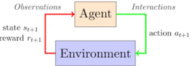
The general reinforcement learning problem formulation has the format of a finite MDP. The interaction between the agent and environment happens at each time-step of a sequence of discrete time-steps, t = 0, 1, 2, 3, ..., where at each time-step t the agent receives a representation of the world - a state, St 2 S, from a set of possible states S, selects an action At from a set of

possible actions A(St) for the state St by implementing a policy ⇡t, where

⇡t(a|s) is the probability that At = aif St= s, and in the next time-step t + 1

the agent receives a reward signal Rt+1 2 R from the environment ending up

in a new state St+1 [3]. The diagram in Figure 1.14 illustrates the interaction

(46)

Figure 1.14: Agent - environment interaction. Image taken from https: // kofzor. github. io/ Reinforcement_ Learning_ 101/

Reinforcement learning methods provide ways to adjust the policy based on the accumulated experience with the goal of maximizing the total cumulative reward in mind. An example for representing the goal in a reinforcement learning problem like that of making a robot learn to walk would be by giving a reward on each time-step proportional to the robot’s forward motion. The reward signal is the way of communicating to the agent what you want it to achieve, not how you want it achieved [3].

A formal definition of the cumulative reward received in the long run is expressed by the expected return Gt, which is a function of rewards sequence

Rt+1, Rt+2, ..., RT received after the time-step t, where T is the last time-step.

In order to express the return more conveniently, the concept of discounting is introduced, which determines the current value of the future rewards. The formula generalized for both episodic and continuing tasks is the following:

Gt= Rt+1+ Rt+2+ 2Rt+3+ ... = T t 1_X

k=0 k_R

t+k+1, (1.9)

where is the discount rate, 0   1. In the case of episodic tasks where there is a terminal state after some time-steps, = 1. For the cases in which the process is continuous and the final step is infinite, T = 1.

With the discounting factor, the reward received after k time-steps has the value k 1 _{times what it would be worth if it were received immediately}

[3]. In the extreme point where = 0, it is said that the agent is myopic, because it only maximizes over the immediate rewards and not the future rewards, whereas if is closer to 1 the agent is far-sighted and sees far into the future considering the future rewards when picking actions.

(47)

The state that has the Markov property represents all the useful informa-tion in order to make a suﬃcient statistic for the future. With Markov states, we have the best possible basis for choosing an action [3]. The environment’s feedback at time-step t + 1 after a particular action was taken at time-step t depends on the events happened before. If the state has the Markov property instead, then the feedback of the environment depends only on that state, because that state represents all the previous events. In this case, the one-step environment dynamics of a finite MDP can be expressed by the following formula:

p(s0, r|s, a) = P r {St+1 = s0, Rt+1= r|St = s, At= a} (1.10)

Based on the formula presented in (1.10) we can also compute the expected rewards for state-action pairs [3],

r(s, a) =E [Rt+1|St = s, At= a] = X r2R rX s0_2S p(s0, r|s, a) (1.11) the state-transition probabilities

p(s0_{|s, a) = P r {S}t+1 = s0|St= s, At= a} =

X

r2R

p(s0, r_{|s, a)} (1.12) and the expected rewards for state-action-next-state triples,

r(s, a, s0) =E [Rt+1|St= s, At = a, St+1 = s0] =

P

r2Rrp(s0, r|s, a)

p(s0_{|s, a)} (1.13)

Value functions estimate how good it is to be in a specific state given the expected return and the policy.

The state-value function v⇡ for the policy ⇡ expresses the expected value

of a random variable given the followed policy ⇡ at any time-step t:

v⇡(s) =E⇡[Gt|St = s] =E⇡ " ₁ X k=0 k_R t+k+1|St= s # (1.14) The action-value function q⇡ for the policy ⇡ is the value of taking an

action a in a state s while following the policy ⇡:

q⇡(a, s) =E⇡[Gt|St = s, At= a] =E⇡ " ₁ X k=0 k_R t+k+1|St = s, At= a # (1.15)

(48)

Value functions have the property of being expressed recursively. The recursive representation is actually the Bellman equation and its solution is the value of v⇡. It represents the basis of diﬀerent ways of computing,

approximating, and learning v⇡. The Bellman equation is kind of a look-ahead

procedure, where the value of a current state is evaluated by looking ahead at the values that future states can oﬀer. It averages over all the possibilities, weighting each by its probability of occurring. It states that the value of the start state must equal the (discounted) value of the expected next state, plus the reward expected along the way [3]:

v⇡(s) =E⇡[Gt|St = s] = X a ⇡(a_|s)X s0,r p(s0, r_{|s, a) [r + v}⇡(s0)]),8s 2 S (1.16) It is a sum over all values of the three variables, a, s0_{, and r. For each triple,}

we compute its probability, ⇡(a|s)p(s0_{, r}_{|s, a), weight the quantity in brackets}

by that probability, then sum over all possibilities to get an expected value[3]. In finite MDPs, an optimal policy ⇡⇤ is the policy for which its expected

return for all the states is greater than or equal to the expected return of all the other policies. There can be many optimal policies, but the evaluation of their optimal state-value functions have the same result. In other words, any optimal policy evaluates to the same optimal state-value function v⇤, which is

presented in the following equation: v⇤(s) = max

⇡ v⇡(s),8s 2 S (1.17)

The optimal action-value function q⇤ evaluates the same for all the optimal

policies as well and it is of the following form: q_⇤(s, a) = max

⇡ q⇡(s, a),8s 2 S, a 2 A(s) (1.18)

Consequently, the optimal value function v⇤ or the optimal action-value

function q⇤ can lead to an optimal policy and these can be found using the

Bellman optimality equations.

The Bellman optimality equation for v⇤ is the value of a state on the

(49)

action for that state [3]: v_⇤(s) = max a2A(s)q⇡⇤(s, a) =E [Rt+1+ v⇤(St+1)|St= s, At = a] = max a2A(s) X s0_,r p(s0, r_{|s, a) [r + v}_⇤(s0)] (1.19)

And the Bellman optimality equation for q⇤ is the following:

q_⇤(s, a) =EhRt+1+ max a0 q⇤(St+1, a 0₎_|S t = s, At= a i =X s0_,r p(s0, r_{|s, a)}hr + max a0 q⇤(s 0_{, a}0₎i (1.20)

For a better understanding of the optimality equations, (1.19) and (1.20), the backup diagrams are provided in Figure 1.15. The backup diagrams illustrate how the update happens by showing the components that are taken into account for the value evaluation.

Figure 1.15: The backup diagrams for v⇤ and q⇤

The Bellman optimality equation generates a system of N non-linear equations, where N is the number of states. It can be simply solved by applying some non-linear methods when the system dynamics (p(s0_{, r}_{|s, a)) are}

known. The solution to the Bellman optimality equation helps in defining the optimal policy; e.g. one can, at any state, choose the action that corresponds to the maximum return, which is also valid in the long term, because the values take into account the reward consequences of all possible future behaviour options [3]. In the case of the action-value pairs, if the system’s dynamics are unknown, then the actions would still be optimal because the agent would choose the actions that would maximize q⇤.

(50)

1.6 Computer Vision

Computer Vision (CV) is a discipline that deals with how computers can be made for gaining high-level understanding from digital images or videos. Computer Vision has a dual goal. It is relevant from biological science point of view, because it aims to come up with computational models of the human visual system, and from the engineering point of view, because of it aims to build autonomous systems which could perform some of the tasks which the human visual system can perform (and even surpass it in many cases). Many vision tasks are related to the extraction of 3D and temporal information from time-varying 2D data such as obtained by one or more television cameras, and more generally the understanding of such dynamic scenes. Of course, the two goals are intimately related. The properties and characteristics of the human visual system often give inspiration to engineers who are designing computer vision systems. Conversely, computer vision algorithms can oﬀer insights into how the human visual system works[100].

1.6.1 History and state of the art

Many researchers involved in Computer Vision agree that the father of Computer Vision is Larry Roberts, who in his Ph.D. thesis (1963) at MIT discussed the possibilities of extracting 3D geometrical information from 2D perspective views of blocks (polyhedra) [100]. Later in that decade, in 1966, MIT involved its students in a summer project, which requires to attach a camera to a computer and having it describe what it saw [101]. Many researchers, at MIT and elsewhere, in Artificial Intelligence, followed this work and studied computer vision in the context of the blocks world. Later, researchers realized that it was necessary to tackle images from the real world. Thus, much research was needed in the so called low-level vision tasks such as edge detection and segmentation. A major milestone was the framework proposed by David Marr (1982) at MIT, who took a bottom-up approach to scene understanding [102] . This is probably the single most influential work

(51)

1.6 Computer Vision 35

in computer vision ever because it has found a paradigm which is not easy to substitute or modify.

In the next years, Computer Vision has grown from studies usually origi-nated from various other fields, and consequently there is no standard formu-lation and no standard solving of the computer vision problem. Instead, there exists an abundance of methods for solving various well-defined computer vision tasks, where the methods often are very task specific and seldom can be generalized over a wide range of applications[100]. Many of the methods and applications are still in the state of basic research, but more and more methods have found their way into commercial products, where they often constitute a part of a larger system which can solve complex tasks.

The major contributor of Computer Vision field has been the robotic application field. In fact, robotics and AI usually deals with autonomous planning or deliberation for system which can perform mechanical actions such as moving a robot through some environment. This type of processing typically needs input data provided by a computer vision system, acting as a vision sensor and providing high-level information about the environment and the robot.

A field which plays an important role for Computer Vision is neurobiology, specifically the study of the biological vision system. Over the last century, there has been an extensive study of eyes, neurons, and the brain structures devoted to processing of visual stimuli in both humans and various animals. This has led to a coarse, yet complicated, description of how "real" vision systems operate in order to solve certain vision related tasks. These results have led to a sub-field within computer vision where artificial systems are designed to mimic the processing and behaviour of biological systems, at diﬀerent levels of complexity. Also, some of the learning-based methods developed within computer vision have their background in biology.

Many of the related research topics can also be studied from a purely mathematical point of view. For example, many methods in computer vision are based on statistics, optimization or geometry. Finally, a significant part