Quantitative assessment of bone quality after total hip replacement through medical images: 2D and 3D approaches

(1)

ALMA MATER STUDIORUM-UNIVERSITÀ DI BOLOGNA

____________________________________________________________

CAMPUS DI CESENA

SCUOLA DI INGEGNERIA E ARCHITETTURA

Corso di Laurea Magistrale in Ingegneria Biomedica

TESI DI LAUREA

in

MECCANICA DEI TESSUTI BIOLOGICI

QUANTITATIVE ASSESSMENT OF BONE

QUALITY AFTER TOTAL HIP REPLACEMENT

THROUGH MEDICAL IMAGES:

2D AND 3D APPROACHES

CANDIDATO

RELATORE

Jonathan Pitocchi Chiar.mo. Prof. Luca Cristofolini

CORRELATORI

Prof. Paolo Gargiulo

Prof. Magnús Kjartan Gíslason

Anno Accademico 2015/16

III° Sessione

(2)

ii

A mio nipote,

Nicholas

(3)

iii

Abstract

Bone quality evaluation is an important step in the clinical field, both in pathological and non-pathological conditions. In particular, in patients undergoing Total Hip Replacement, the presence of the prosthesis alters the physiological stress conditions of the femur, causing a process of bone adaptation that can have consequences on implant stability and bone conditions. Therefore, it is evident the importance of monitoring the quality of the bone surrounding the stem, both in short and long term period.

Starting from densitometric measurements on CT images, this thesis tackles two main topics: 1) improvement of current protocol to evaluate bone mineral density changes (three-dimensionally around the prosthesis) 1 year after the operation and application to a large dataset (11 patients) to examine the differences between subjects; 2) feasibility study on 8 patients of novel 2D approaches based on standard cross-sectional slices of femur, in order to obtain a tool for bone quality evaluation which can be affordable for the clinicians, but also minimally invasive for the patients, by reducing the radiation dose.

The results of the 3D approach suggest that it may be used as a monitoring tool during the follow-up. Moreover the thesis shows the feasibility of the new 2D approaches, although some limits need to be overcome to use them in a clinical ambit.

Keywords: Total Hip Replacement; Bone Remodeling; Bone Mineral Density; 2D and 3D assessment; Bone profile.

(4)

iv

Abstract

La valutazione della qualità dell’osso è un passo importante nel campo clinico, sia in condizioni patologiche che non patologiche. In particolare, in pazienti sottoposti ad intervento di sostituzione totale d’anca, la presenza della protesi altera le condizioni di stress fisiologiche del femore, causando un processo di adattamento dell’osso che può avere conseguenze sulla stabilità dell’impianto e sulle condizioni dell’osso. Perciò, è evidente l’importanza di monitorare la qualità dell’osso che circonda lo stelo, sia nel breve che nel lungo termine.

A partire da rilevazioni densitometriche effettuate su immagini TC, questa tesi affronta due argomenti principali: 1) miglioramento del protocollo corrente per la valutazione della variazione di densità minerale ossea (tridimensionalmente attorno alla protesi) dopo un anno dall’operazione e applicazione ad un ampio dataset (11 pazienti) per esaminare le differenze tra soggetti; 2) studio di fattibilità su 8 pazienti di nuovi approcci 2D basati su sezioni standard del femore, con lo scopo di ottenere uno strumento per la valutazione della qualità dell’osso che possa essere affidabile per i clinici, ma anche minimamente invasivo per i pazienti, riducendo la dose di radiazione.

I risultati dell’approccio 3D suggeriscono che può essere usato come strumento di monitoraggio post-operatorio del paziente. Inoltre la tesi mostra la fattibilità di nuovi approcci 2D, sebbene alcuni limiti devono essere superati prima di poterli utilizzare in ambito clinico.

Parole Chiave: Sostituzione Totale d’Anca; Rimodellamento Osseo; Densità Minerale Ossea; Valutazione con approcci 2D e 3D; Profilo Osseo.

(5)

v

Overview

Bone quality evaluation is an important step in the clinical field, both in pathological and non-pathological conditions. Having a better knowledge on how the bone is adapting to different situations, can strongly improve the diagnostic phase, helping clinicians in the decision making. Nowadays, there are different cases in which medical images are used to assess the quality of bone structures, e. g., DEXA has become the standard technique to quantify Bone Mineral Density, providing an accurate method to diagnose osteoporosis. More recently, many studies have shown how qCT (quantitative Computed Tomography) can be the starting point in the analysis of damaged or diseased tissues [1] [2] [3] [4].

In this interesting field, most current research is focusing on improving the aspects of instrumentation design, image processing software, data acquisition procedures and computational modeling, to obtain a tool which can be affordable for the clinicians, but also minimally invasive for the patients, by reducing radiation dose.

With regards to the main subject of this work, similar remarks may be made about the evaluation of bone quality in subjects undergoing Total Hip Replacement (THR). This orthopedic surgical procedure is one of the most used and most successful in the world, restoring the functionality of the hip-joint articulation and increasing life expectancies [5]. THR consists of replacing the acetabulum and the femoral head with two different components. There are two methods to perform the operation: in the first case, bone cement is used to fix the prosthesis (CEMENTED), instead in the second one, a press-fitting procedure allows the primary stability between implant and bone (UNCEMENTED). Although this operation offers immediate free movement and pain-relief, many clinical problems are highlighted in the literature. The presence of the prosthesis in fact alters the physiological stress conditions of the femur, causing a process of bone adaptation that can have consequences on implant stability.

Many factors are involved in the mechanism of bone remodeling: these includes not only patient-related factors (such as gender, patient activity, general health), but also prosthesis-patient-related factors (type of fixation, geometry of the implant, position). Based on these considerations, it is evident the importance of monitoring the quality of the bone surrounding the stem, both in short and long term period. [6]

(9)

2

This thesis is part of a large project [7] involving Landspítali – University Hospital of Iceland and Reykjavík University, that aims to introduce novel approach, acquire unique data and suggest patient specific evaluation to optimize implant technology and clinical assessment. As a result of this collaboration, a protocol to evaluate bone mineral density changes around the prosthesis one year after surgery has been already created and qualitatively validated. [8]

Through this process, unlike every other technique carried out to study bone density changes (like DEXA), it is possible to have volumetric measures of bone growth/loss and to see how these changes are distributed in the bone’s model. Anyway, such a method requires access to the full-bone CT-scans acquisition, both for Post24 and Post1y dataset, thus limiting its applicability in the clinical field. For these reasons, the possibility to extract the same information from single, standardized slices, is a main goal to pursue, both for clinical advantages and ethical issues.

This thesis tackles two main topics: 1) improvement of the previous protocol for 3D gain/loss evaluation and application to a large dataset to examine the main differences between subjects 2) feasibility study of novel 2D approaches based on standard cross-sectional slices of femur.

For the 2D approach, 5 CT-scans are selected (both for dataset Post24 and Post1y) and then examined in two different ways:

a) Gain/Loss assessment using Matlab Image Processing Toolbox: using the image process toolbox of Matlab, it is possible to overlay the images and replicate the 3D approach, showing, just in the slice, how Bone Mineral Density (BMD) changes 1 year after the operation. This method is potentially easier to apply in the clinical field, especially in the region of the femur where bone gain and loss are greater.

b) 2D Bone Profile: through a model fitting of the Density Distribution of the 5 CT-scans (HU-n° of pixels), it is possible to extract some parameters that can be used for bone quality assessment.

(10)

3

1. Introduction

The main purpose of this chapter is to introduce the basic information about the anatomy and the biomechanical properties of bones and the nature of THR surgery. Moreover, the fundamental principles of Computed Tomography are described in order to better understand the procedures analyzed in the thesis, along with its purpose in bone quality assessment.

1.1 The Bone

1.1.1 Bone Physiology

Bone is a specialized form of connective tissue in which the extracellular matrix is mineralized, thus conferring stiffness and mechanical strength to the skeleton while still leaving some degree of elasticity. Although it is a living tissue, it is composed (on a weight basis) by 2/3 of inorganic component (such as calcium carbonates and phosphates) and by 1/3 of organic component (principally collagen, but also lipids, proteoglycans and cells). The organic part is the tough and flexible component while the mineral is the brittle and stiff one.

The bone has two important and distinct functions:

-physiological function: it acts as a mineral reservoir for calcium homeostasis, in order to keep constant its level in the blood under different physical and metabolic activity; moreover, it provides an environment for marrow (both blood forming and fat storage),

-mechanical function: it protects the vital organs and, in synergy with muscles, consents the motion of the entire body.

Bone has a strongly hierarchical organization. (Fig 1.1)

Focusing on a nanostuctural scale, it is possible to distinguish the presence, within the collagen fibrils, of little crystals of hydroxyapatite (HA), namely calcium apatite, Ca10(PO4)6(OH)2, (length: 20-40 nm; thickness: 1.5-5 nm) pointed on the same direction of the collagen fibers, thus influencing the mechanical properties of the bone. At a microscopic level, parallel collagen fibers are organized into layers called lamellae (thickness: 3–7 μm). Lamellae put near each other have different orientations, building a ply-wood like structure.

(11)

4

In the cortical bone, a group of 4-20 concentric lamellae are arranged to surround a central cavity, the Haversian canal (which contains vessels and bone nerves), forming a cylindrical system called osteon (with a diameter of 150-250 μm). [9]

Fig. 1.1: Hierarchical levels of the cortical bone [10]

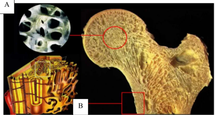
The highest hierarchical level includes two main bone types: cortical (or compact) and trabecular (spongy or cancellous). (Fig 1.2) One of the difference is linked to the contents of marrow and soft tissue: less than the 10% of the volume in cortical bone, almost the 75% of volume in cancellous bone.

Fig. 1.2: Trabecular (A) and Cortical (B) Bone in proximal femur

Image 1.2 shows also a substantial diversity between the two organizations, thus influencing the mechanical properties. Cortical bone is dense and consists of aligned osteons while trabecular bone is highly porous with spongy appearance in which lamellae are arranged in small struts called trabeculae (thickness < 0.2 mm). Cortical bone is heavier, stiffer and stronger, while trabecular one is lighter, less dense and with low mechanical strength properties.

A

(12)

5

1.1.2 Bone Remodeling

Bone remodeling is the complex of concurring biological process that lead to bone geometry and bone density changes. The first analysis of this mechanism is attributed to Julius Wolff who proposed a mathematical formulation (Wolff’s law) to describe how the bone adapts and forms its architecture according to the externally loads applied, in order to maintain a physiological stress-strain state. (Fig. 1.3)

Fig. 1.3 Possible phenomenology of bone remodeling. Adapted from [11]

Figure 1.3 shows a possible phenomenology of bone remodeling, as a result of a mechanical stimulus. Considering that σ is the stress in the resistant section following an applied force and ε the associated strain, if the strain is above or below a threshold defined by the physiological levels, bone starts a process of adaptation which leads to a prevalence of growth or resorption. In particular, if ε is under a minimum value, cortical bone’s thickness decreases in order to have a smaller resistant section and trabeculae’s number and dimension are reduced, along with a demineralization of the matrix (resorption). On the other hand, if ε exceeds a maximum value, bone remodels in the opposite way (growth).

(13)

6

This process is always present and is fundamental not only for removal and repair damaged bone, but also to maintain integrity of the adult skeleton and mineral homeostasis. [12]

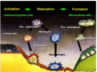
The mediators of bone remodeling are the cells that populate bone tissue. Osteoblasts (mono-nuclear) can be stimulated to increase bone mass. They are able to synthetize and release a non-mineralized matrix, called osteoid. Osteoclasts are the only cells capable of resorbing bone. They are typically multinucleated and can attack HA through an acidification of the environment. Osteocytes can be defined as the sensors of the process. They are former osteoblast trapped in the just produced osteoid and lead the action of osteoblasts and osteoclast. The remodeling is obtained with a continuous process in which osteoclasts reabsorb old bone and osteoblasts create new matrix. Main steps are shown in figure 1.4.

Fig. 1.4: Activation, Resorption, Formation in bone remodeling

First osteoclasts are activated, thus starting the resorption phase that lasts approximately 10 days. Following resorption, macrophage cells are present in the remodeling site. Pre-osteoblast are then recruited. After the differentiation in mature osteoblasts, they begin to secrete new osteoid matrix that then mineralizes to form new bone. The complex balance between bone resorption and formation is guided by interrelated factors such as genetic, mechanical, vascular, nutritional, hormonal, and local. [13]

Bone remodeling allows the human skeleton to adapt to different load situations. In particular, looking to the arrangement of cortical and trabecular bone in the proximal femur, it is possible to see how, especially the trabeculae, are optimized to resist to the daily forces conditions. Moreover, the epiphysis can absorb a great amount of energy in case of an impact due to a sideway fall. (Fig. 1.5) The alignment of osteons and trabeculae respond also to a metabolic necessity: in fact at this

(14)

7

arrangement correspond at the same time a minimum amount of material and a minimum risk of damage.

Fig. 1.5 Direction of stresses created by body weight, muscles forces and joint force Copyright McGraw-Hill Companies, Inc

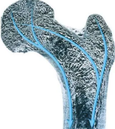
Focusing on the effects of a total hip replacement on this optimization, it is clear that the presence of the stem (which is much stiffer than the surrounding bone), modifies the loading conditions with respect to the preoperative situation. The principal consequence is an alteration, induced by the metal implant, of the normal stress patterns that lead the bone remodeling. This phenomenon is called stress shielding. Figure 1.6 shows how load is transferred from the pelvis to the femur after THR. The stress-shielding leads to an imbalance of the bone remodeling, causing bone resorption around the stem, because the metal shields the bone from the stresses, potentially compromising implant stability [15]. At the tip of the stem instead there is not a demineralization and, on the contrary, bone growth is encouraged (the prosthesis transfers the load it is subject).

Fig. 1.6 Image showing how load is transferred from the pelvis to the femur after THR. The stem is stiffer than the bone, this causes stress shielding in the proximal femur, with consequent bone mineral density decrease.

(15)

8

1.1.3 Anatomy of the femur

The femur belongs to the category of long bones and it is the longest between the 206 bones in the adult skeleton.

As shown in fig. 1.7, it typically consists of a central part, tube-shaped, called diaphysis, in which a shell of cortical bone surrounds the trabecular one.

Fig. 1.7: Anatomy of the femur

Approaching the joints, an intermediate region, the metaphysis, connects the diaphysis to the epiphysis, covered by articular cartilage (hyaline) that allows the relative movement of adjacent bone segment, reducing the friction between the surfaces.

The outer layer of the cortical bone is called periosteum. It contains active cells that enlarge the diameter of bones in remodeling.

The canal in the middle of long bones is called the medullary canal. The surfaces of these canals are called endosteum, which mainly consists of laminated cells. [10] Also in the endosteum the remodeling is strong hence having a pivotal role in bone-formation.

(16)

9

1.1.4 The Hip Joint

The hip joint (coxal) is one of the most important and most flexible joint in the human skeleton. It is a synovial ball-and-socket which connects the lower limb to the pelvic girdle.

The ball is the head of the femur (hemispherical) which fits into the acetabulum (a cup-shaped socket in the pelvis). As a joint cavity, the touching surfaces are covered with articular cartilage, providing a smooth surface for the movement of the bones; moreover, it has a synovial membrane producing synovial fluid. (Fig. 1.8)

The presence of strong muscles and ligaments that connect the ball to the socket leads to a great stability of the joint. In this way, it can transfer the loads to the legs both in static (e.g. standing) and dynamic (e.g. walking) postures. Especially during running and jumping, the force of the body’s movements multiplies the force on the hip joint to many times the force exerted by the body’s weight. The hip joint has to be able to resist to these extreme forces repeatedly during intense physical activities.

Biomechanically, the hip joint has a very high range of motion. The ball-and-socket structure allows flexion/extension, abduction/adduction and medial/lateral rotation.

(17)

10

1.2. Total Hip Replacement (THR)

1.2.1 Introduction

Total Hip Replacement is one of the of the most common surgery done on the human musculoskeletal system today and with increasing life expectancies in many populations worldwide, also the number of operation will continue to raise. [5] Its success is also due to the fact that it offers immediate free movement and pain-relief, restoring the functionality of the hip joint.

There are different reasons which cause subjects to undergo a THR. For example, in a study from 2001 that involved 101 patients, frequent complaints were: walking (68%), pain (58%), limping (36%), night pain and walking stairs (both 35%) [17].

Looking in the literature for the medical condition that usually lead to THR, one of the most common diagnosis is osteoarthrosis (OA). [18] [19] OA is a wear-related type of joint disease, generally found in elderly people. It consists of a mechanical breakdown of the cartilage which is linked to sever pain during daily living activities. OA affects the entire joint, but the part that principally suffers is the articular cartilage that allows the femoral head to moving into the acetabulum without friction. Other diseases requiring THR include: Rheumatoid arthritis (AR), where the cartilage is damaged because of chronic inflammation; Avascular necrosis, where blood supply to the femoral head is limited, causing the bone to collapse; Paget’s Disease, a metabolic bone disorder that induces an increased and irregular formation of bone; Developmental Dysplasia, in which femoral head has an abnormal relationship to the acetabulum; Tumor; Femur’s neck Fracture. [20]

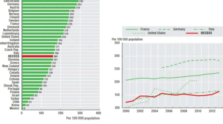
The popularity of this surgical operation is confirmed by study on the population undergoing THR. (Fig 1.9)

The statistics from Emilia Romagna (Italy) [19] and the rest of the OECD countries [21] show that the number of hip replacements has augmented rapidly since 2000. On average, the rate of hip replacements increased by about 35% between 2000 and 2013.

(18)

11

Fig. 1.9. Left: Number of THR surgeries in 2013. Iceland counts 185 operations per 100 000 people, Italy 166; Right: Trend in hip replacement surgery, for some selected countries, from 2000 to 2013. Average statistics for OECD countries are represented in red.

Analyzing the data collected between 2000 and 2014 in Emilia Romagna, the average age for the first THR was 66.7 years.

The majority of the subjects who received the implant is female (60% of the patients undergoing THR during the period 2000-2014). The statistics highlight also that the average age for male was 66.5 while for female was 70.2.

(19)

12

1.2.2 Prosthesis Components and Surgery

Prosthesis for THR have been the object of a continuous research in order to limit the complications after the surgery, this way leading to a large variety of stems on the market, classified according to shape, material, coating etc. Today however, it is possible to define a basic modular-design common for all the implants. (Fig. 1.10)

The prosthesis is generally composed by two modules: the hip one (shell + liner), anchored to bone of the pelvis and the leg one (femoral head + femoral stem), which is inserted in the femur.

The liner is put into the shell to allow a smooth movement between the surfaces. This component represents the socket of the artificial joint. The femoral head instead is the ball and it rotates within the liner.

(20)

13

Currently, there are two methods used to fix the implant: with cement (cemented) and through press-fit (uncemented).

Fig. 1.11 (A) Femoral neck removal [23] (B) Articular cartilage in the acetabulum removed with reamer [24] The surgical operation follows standard steps. Firstly, the femoral head and part of the neck is removed (osteotomy, Fig. 1.11, a). Regarding the hip preparation, a rasp/reamer is used to clean the articular cartilage thus leading to securely fix the acetabular component. (Fig. 1.11, b)

At this point, femur needs to be prepared to receive the stem. The procedure differentiates for cemented and uncemented approach.

For cemented implant,the stem is fixed through an acrylic bone cement. In general, the material for the cement is Polymethylmethacrylate (PMMA). The surgeon, using a reamer, creates a cavity into the femur, he removes the spongy bone in the medullary canal, then he compresses and removes the bone with a rasp. At the beginning, smaller rasp sizes are used until templated size of the stem is reached. The final size of the rasp is bigger than the stem to leave space for cement. [23] Moreover, a bone plug (called cement restrictor) is inserted into the canal to prevent the cement from flowing along the distal part of the femur.

Bone cement is injected into the prepared femoral canal. In this phase, it is extremely important that the cement is distributed in a homogenous way, in order to avoid implant loosening and to decrease the risk of periprosthetic fractures. Having stem with smooth surface helps the success of the surgery, cause local peaks of stress may lead to cracks in cement layers. (Fig. 1.12)

(21)

14

Figure 1.12: Cemented implant (left). Uncemented implant (right) [25]

For uncemented implant, the press-fit contact between implant and surrounding bone is employed to anchor the stem (Primary stability). Additionally, the induced bone ingrowth into the porous surface of the prosthesis leads to a more solid fixation (Secondary stability). (Fig. 1.12)

The surgeons, through hammering blows, fixes and inserts the stem. He needs to be really carefully in terms of force, since an excessive load may result in a fracture.

1.2.3 Comparison between Cemented and Uncemented Implant Fixation

After a brief description of THR surgical procedure and of the two typologies of implant fixation, it is necessary to examine how the femur is affected by the presence of the prosthesis. In this way, it is possible to highlight the importance of the bone quality assessment not only in the pre-operative decision making, but also in the follow-up of the patient.

In fact, despite the success of both cemented and uncemented implant, today there is not an absolute criterion for choosing between these methodological options. Utilizing the cemented approach provides a better primary stability, thanks to the presence of a cement layer between the implant and the bone. Moreover, the presence of the cement reduces the stress-shielding.

Anyway, the bone resorption generated by stress-shielding increases the periprosthetic fracture risk and can lead to stem’s aseptic loosening, which is reported as one of the major reason for implant failure. [26] [27]

(22)

15

On the other hand, without the use of cement, prosthetic primary stability is achieved thanks to the geometrical inter-locking, the press-fit and the friction between femur and stem, while secondary stability is secured by the bone adaptation of the layers adjacent to the prosthesis. In fact they are preloaded and this stress encourage a process of bone growth into the surface texture of femoral component (osteointegration). [28]

Although the continuous research in this field, because of the great number of implants, many subjects undergoing THR need revision 10 or 15 years after the operation. In the first years post-operatively instead, non-cemented implants are more frequently revised, due to the periprosthetic fracture. Anyway, the revision surgery for press-fit procedure is easier, with fewer complications than revision surgeries for cemented implants. [29] [30] In fact, when the prosthesis and the cement are removed, a part of the inside of the femur follows, thus having bad consequences on bone strength.

Considering the revision rate for infection instead, similar outcomes are shown for both the uncemented and the cemented fixation with antibiotic cement. [31]

As described in § 1.2.2, a critical phase during press-fit is when the surgeon hammers the stem into the bone. It is important that the clinicians check bone quality because with a low bone mineral density or an important disease (like osteoporosis) the bone may not be able resist to the forces produced with the hammering, thus leading to an intra-operative fracture. For this reason, uncemented implant is usually chosen for younger and more active patients, while for older and less active patient the cemented option is more safe. Anyway, other factors have an impact the decision making, such as gender, bone mineral density, stem design, gait patterns.

1.3 Basic principles of Computed Tomography

Computed Tomography (CT) has become through the years a very powerful tool in medical imaging, using X-rays to provide an image that is based on the linear absorption coefficients of the tissues through which they pass. In this way, it is possible to obtain a series of cross-sectional slices of the body in which distinguish different structures depending on their density. Every CT image is the result of two different steps: first scan data acquisition and then tomographic reconstruction trough computational processing. [32] [33] [34]

(23)

16

The image is acquired by a rapidly rotating x-ray tube around the patient. The radiation that is not absorbed by the body is measured by detectors and the final image is generated by reconstruction from the multiple x-ray projections through complex algorithms. (Fig. 1.13)

Fig. 1.13: Simplified schematic image of CT data acquisition

All CT images are formed by voxels, which are volume elements. Every voxel is described by a CT value. It is the average value of all linear attenuation coefficients and reflects how much the energy of the x-ray beam is reduced when going through the tissue, contained within that particular voxel. Since the attenuation coefficients can vary between CT scan models and different settings on the same scanner, the Hounsfield Unit scale (HU) is used to standardize them. The HU is defined based on the attenuation coefficient of each voxel, compared to attenuation coefficient of the water and of air as described by formula 1.1.

X Water

Water Air [1.1]

X is the average attenuation coefficient of the voxel, Water is the attenuation coefficient of water and Air is the attenuation coefficient of air. The Hounsfield Unit scale is based on a normalized index where air is defined to have value of -1000 HU and water the value of zero HU. Since attenuation depends on the density of the scanned volume it is possible to distinguish between hard and soft tissue is possible.

(24)

17

Moreover, calibrating the CT scanner with a phantom allows to define the relationship between HU and BMD, as it will be examined in § 2.1.3.

One voxel can contain different types of tissues due to the finite spatial resolution of the imaging tool. This phenomenon generates the so-called partial volume effect (PVE). Regarding this work, PVE is one of the main problem during the segmentation process. In fact, at the interface between a softer and a harder tissue (i.e. cortical bone and muscles) the edge may appear as blurred and it is more difficult to separate the tissues.

1.4 Bone quality evaluation

As already explained, bone quality plays a pivotal role in the success of THR. Clinical assessment of bone material distribution is an important factor in determining the treatment for patients or to monitor the changes in bone quality over a period of time. It is inevitable that the bone will undergo changes in morphology and strength following a THR procedure. It is however important to be able to monitor where the changes occur to determine if the bone density decreases (loss) or if it increases (gain). Along with mechanical test [35] [36], different approaches based on medical images are becoming very useful, giving the possibility to extract information to improve planning and post-operative assessment.

Measuring bone mineral density in vivo for example, can provide quantitative information on bone’s quality, that can be used for several applications. Along with plain radiographic absorptiometry and dual energy X-ray absorptiometry (DEXA), quantitative computed tomography (CT) represents a good tool to measure BMD. In fact, quantitative CT is the most reproducible and accurate method for in vivo assessment of cortical and cancellous bone density. [37] [38] Moreover, is the only technique that provides a three-dimensional volumetric analysis, since it provides a series of cross-sectional images.

Starting from CT-scans, it is possible, through a standard segmentation based on opportune threshold of the CT-HU, to separate bone from other tissue and apply noninvasive approach to measure BMD. This procedure can be used in different way, giving the possibility to monitor density changes both in healthy and operated leg of the same patient and differentiate the results by implant technique and gender versus subject’s age. [39]

(25)

18

Similar analysis it’s critical in the pre-operative evaluation, in order to optimize prosthesis selection. As already described, clinicians have not guidelines when choosing between cemented or uncemented procedure, so usually they rely on experience or simple patient metrics such as age and sex. Different studies show that such information alone is not enough for providing optimal decision on the implant technology to employ, highlighting the importance of a correct evaluation of BMD. [40] [41] [42] [43]

1.5 Aim of the thesis

An approach based on CT-scans offers different modality to evaluate bone quality, not only in the THR field. However, in comparison to another standard method, such DEXA, subjects undergo higher radiation dose (0.5-1.0 mSv against 0.001-0.1 mSv). [44] This may represent a limit in the clinical application, cause, especially today, there is an increasing need to obtain tools that are affordable but also minimally invasive for patients.

For this reason, the principal aim of the thesis is to investigate novel 2D approaches, using standard CT-scans acquired 24 hours and 1 year after total hip arthroplasty, in order to create an ethically compatible method that can be used in the clinical field to examine bone quality

After performing an improvement of the 3D evaluation for BMD changes developed at Reykjavik University, the protocol is, for the first time, applied to a set of cemented patients. This way, a comparison between the volumetric bone growth/loss in subjects with different type of implant fixation is possible, increasing the number of application of the method.

Moreover, through a selection of 5 slices in the regions of interest of the femur, a new technique based on the analysis of the Density Distribution of the CT-scan (HU values-N° of pixels) is applied to 8 uncemented subjects. The results have been compared to the 3D approach, showing the outcomes of such approach and determining advantages and disadvantages of each method.

The slices of the same 8 patients have been also processed with an alternative procedure which allows to visualize and quantify the bone gain/loss in single images through a more automated image registration provided in Matlab.

This thesis wants to test the feasibility of a bone quality assessment based on few slices, moving the first steps to make this kind of investigation more sustainable both for clinicians and patients.

(26)

19

2. Materials and Methods

This section contains all the steps needed to reproduce the analysis with other subjects in the future. The chapter is divided in four parts. In the first one are presented the information about subjects involved and protocol of acquisition (CT-scan, CT-calibration, Metal artefact reduction). Then, three different protocol for the assessment of bone quality are described, along with the tools used in the evaluation.

2.1 Data

2.1.1 Subjects Information

Currently, a total of 75 patients are enrolled in the project of the RU named “Clinical evaluation score for Total Hip Arthroplasty planning and post-operative assessment”. The criteria for being included were that patients could not have had a previous THA or total knee arthroplasty (TKA). Anyway, for this study, 11 subjects have been selected from the entire cohort, 7 females and 4 males. 8 received an uncemented implant, 3 a cemented one. The youngest patient was 48 years old and the oldest 65. The implant selection for the patients was in the hands of their operating surgeon who based their selection on patient’s age, gender and general physical conditions.

The average age is 56.3 ± 6.6 years. For males, the average age is 51.8 ± 5.6, while for females the average age is 58.9 ± 6.0 years. All the information about patients’ gender, age and type of implant are summarized in the Table 2.1.

Table 2.1: Patient’s info

Patient n° Age Sex Type of implant

1 60 F Uncemented 2 48 F Uncemented 3 50 M Uncemented 4 61 F Uncemented 5 48 M Uncemented 6 49 M Uncemented 7 54 F Uncemented 8 60 M Uncemented 9 60 F Cemented 10 64 F Cemented 11 65 F Cemented

(27)

20

2.1.2 CT Acquisition

All the subjects were scanned with a Philips Brilliance 64 Spiral-CT (Fig. 2.1) three times: 1-3 days before, 24 hours and 1 year after the surgery. However, for the purpose of this project, only 24h and post1y dataset was utilized.

The scan protocol included slice thickness of 1 mm, slice increment of 0.5 mm and a tube intensity of 120 KVp.

Fig. 2.1: Philips Brilliance 64-slice CT scanner

The slice increment determines how much the gantry moves forward each circle and if it is shorter than the slice thickness, overlapping occurs, thus increasing the quality of the slices. This imaging protocol allowed an accurate 3D reconstruction of the femur from the iliac crest to the middle of the diaphyseal femur. (Fig 2.2)

(28)

21

2.1.3 CT calibration

Prior to the study, in order to get the mathematical relationship between HU of pixels and BMD (g/cm^3), the CT scan was calibrated with Quasar Phantom [45], enclosing different materials. The resultant of the calibration can be seen in the figure below (Fig. 2.3):

Fig. 2.3: BMD vs. HU relationship

Here instead the resulting formula [2.1]:

(29)

22

2.1.4 Metal artefact reduction

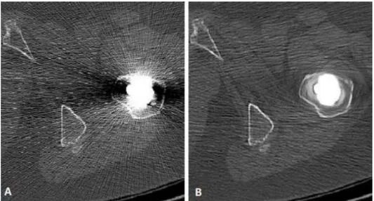
Due to the presence of the prosthesis, the Post24 and Post1y dataset is strongly affected by metal artefact. The streaks derived from the implant change the HU of pixels of normal body tissue. In some cases, this artefact can significantly alter the values in the region of interest involved in this study. For this reason, the images are processed with the software Metal Deletion Technique from ReVision Radiology [46].

As explained in [47], the Metal Detect Technique (MDT) discards the inaccurate metal data and only uses the good quality ones to reconstruct the non-metal portion of the image. This process iteratively performs forward projection to replace detector measurements that involve metal. The result of MDT is shown in the figure below (Fig. 2.4).

(30)

23

2.2 3D Gain/Loss assessment

In this section, a method for the 3D evaluation of BMD changes is described. The protocol provides qualitative and quantitative information about gain and loss in patient undergoing THR, 1 year after the surgical operation. This protocol is applied to all the 8 uncemented patients and, for the first time, to 3 subjects with cemented fixation.

2.2.1 Study Workflow

Fig. 2.5 Study Workflow

The assessment methods are based on CT-scans acquired from patients undergoing THR at 3 different times: before operation, post 24 hours and 1 year post operation. The post 24 hours and the post 1 year images are processed, reconstructed in 3D, registered and compared; this way, the 3D evaluation of gain and loss after 1 year from THR is achieved. The same data are used, through a selection of standard slices, to implement the 2D approach.

2.2.2 Bone segmentation

In the 3D gain/loss protocol, the bone mask (set of pixels selected on the image) is obtained by a semi-automatic process.

After importing the CT-scan in Mimics®, performing segmentation, it is possible to separate the real bone from other tissues. This step is fundamental for the workflow, cause the analyses will involve this mask.

(31)

24

The “3D Live Wire” segmentation tool uses contour lines to manually follow the femur in the images. This is done every 5 to 10 slices depending on how the bone appeared, in both sagittal and coronal planes. The result of this could be reviewed in the axial plane before the segmentation. (Fig 2.6)

Fig. 2.6: The 3D Live Wire Tool workflow. First, contour lines were manually added between 5 to 10 slices in coronal and sagittal view. Contours were reviewed in the axial view. After that, the tool segmented the femur. Then, 4 pixels are eroded from the bone mask.

A Boolean operation (Minus) between the bone mask and the eroded one, allow to have a “shell” that, basing upon previous studies, represents the external layer of the compact bone [48].

Separately, another mask is created through a threshold on the HU. In particular, 255 HU is set as the lowest value for the cancellous bone, while 3070 is considered as the highest value for the cortical bone.

This mask is then added (Boolean operation: Unite) to the “shell”, thus having a unique mask in which apply the gain/loss evaluation, called “contour”.

Using a unique threshold (3071 HU), the prosthesis is also segmented. A Boolean operation (Minus) is applied to the contour mask in order to separate the bone from the implant. (Fig. 2.7)

Finally, additional manual fine tuning is done to get rid of artifacts, e.g. due to stem’s metal. The same process is repeated both for Post24 and Post1y dataset.

(32)

25

Fig. 2.7: 3D model of contour mask as result of the segmentation

2.2.3 Reslicing

Image registration is needed to align the two datasets so that the femur is in identical position between the scans. Anyway, although CT scanner machine and its settings are the same during the acquisitions (Post24 and Post1y), patient’s lower limb can be rotated with different angles, thus complicating the assessment of gain/loss in the corresponding areas of the bone.

Through the Reslice Project Mimics it is possible to align the orientation of the body to have a better images registration. Moreover, with this step, pixel size of the two images is uniformed, since it is possible to define it during reslicing. Through a similar process, both Post 24h and Post 1y are resliced following a common line, in this case the longitudinal axis of the stem, which can be selected in the coronal view. Pixel size modification is applied to one of the two images, namely that with the highest value (lowest resolution). Its pixel value is modified setting it to other image’s one, i.e. to the lowest value (highest resolution). Reslicing is also important to crop the area of interest of the femur, i.e. the proximal part, from the whole image for an easier analysis. (Fig. 2.8)

(33)

26

Fig. 2.8: Reslicing procedure

2.2.4. Image Registration

As already mentioned, for a correct evaluation of BMD changes, the 2 datasets need to be registered to compare the same zones of the bone.

In Mimics, a point-based registration is available to overlay the CT-scans, so this process is carried out identifying 6 points belonging either to the femur or the stem and considering anatomical landmarks which are easily recognizable (Fig. 2.9). These reference spots are:

a) Stem´s tip

b) Protuberance under greater trochanter (distal end of the attachment site for gluteus minimus) c) Top of greater trochanter

d) Lesser trochanter

e) Gluteal tuberosity in axial view

(34)

27

Fig. 2.9: Landmarks for point-based Registration

Additionally, it is possible to add more landmarks to improve this procedure, although it is strongly recommended to use points belonging to the femur and not to the prosthesis or pelvis bone (except for suggested landmark a).

In the Image Registration tool, the Subtract Fusion Method is then selected. This way, while the scans are registered, a voxel by voxel intensity subtraction is performed. As result, a new Mimics project is created in which the GVr (resultant GrayValue) of a generic voxel is obtained by the difference between the GV of the correspondent voxels in the 2 datasets (GV1-GV2).

Since Mimics’ Subtract Fusion Method sets to “black” (GVr = 0) all the voxels with either negative or null GVr, assigning a certain level of gray only if GVr is positive, one registration + subtraction procedure is made to evaluate bone gain, while the other one is made for bone loss. (Table 2.2)

Table 2.2: Subtract Method

(35)

28

2.2.5. Bone Gain/Loss evaluation

Once that the registration is complete, gain and loss in the femur are evaluated both quantitatively and qualitatively. The below-described steps are separately applied to each new Mimics Project, therefore bone resorption and bone growth are independently evaluated (as explained in Table 2.1). First of all, the masks of the Post 24h and Post 1y femurs are imported (see § 2.2.2) in order to consider just the interesting pixels belonging to the bone.

The main source of error affecting a precise BMD changes assessment is the misalignment between the two registered datasets. A solution to this problem is to erode 3 pixels from the imported bone masks. This way, part of the outer femur is not considered in the comparison between Post 24h and Post 1y bone mineral densities.

Moreover, to examine significant BMD change only, a Threshold Mask is created having 111 GV as lower limit, according to the previous protocol. This corresponds to the minimum significant value of BMD change, meaning that a GVr loss (or equivalently a GVr gain) lower than 111 is not considered to be relevant.

Successively, by doing a Boolean operation of Intersection between the Eroded Femur Mask and the Threshold Mask, the Final Loss (or Gain) Mask is achieved.

Checking the mask properties, information about the volume (mm3) of bone lost (or gained) is obtained, along with the volume of the femur mask. This way it is possible to calculate the percentage of lost and gained volume 1 year after THR using the following formulas [2.2, 2.3]:

%

=

×100

[2.2]

(36)

29

Finally, a three-dimensional representation of the loss/gain areas over the proximal femur is realized, to better understand where the changes have occurred.

(37)

30

2.3 Cross-section based assessment

In order to define an ethically compatible method to assess bone condition, two different procedures are described, based on the selection of 5 standard CT-scans. The first one utilizes Matlab Image Processing Tool to obtain information about gain and loss in single slices. The second one instead aims to introduce a strong method to extract a distribution (HU values-N° of pixels) from the image which can be used to study bone quality.

2.3.1 Selection of standard CT-scans

Cause standard cross-sectional slices are needed to apply the 2D approach, five CT-scans were selected from the dataset, according to the work of Pitto et al. [49]. Listed from the most proximal to the most distal, the 5 regions of interest are: 1) greater trochanter; 2) lesser trochanter; 3) 5 cm proximal to stem’s tip; 4) stem’s tip; 5) 2 cm distal to stem’s tip. (Fig. 2.11)

Fig. 2.11: 5 Regions of Interest for BMD: 1) Greater Trochanter, 1) Lesser Trochanter, 3) 5 cm proximal to stem’s tip, 4) stem’s tip, 5) 2 cm distal to stem’s tip. F) Coronal view.

These CT-scans have been chosen also because they are easily detectable in both Post24 and Post1y dataset. Moreover, these slices define 5 volumes of interest in which BMD changes can be evaluated

(38)

31

by the 3D assessment (using formulas [2.2, 2.3]), providing interesting information on how the gain and loss is distributed in each sub-volume. (Fig. 2.12)

Fig. 2.12: 5 sub-volumes of the 3D femur

2.3.2 Gain/Loss assessment using Matlab Image Processing Toolbox

In this paragraph, pursuing the same target of the 3D gain/loss analysis, a new approach based on the registration of 2 slices of the same ROI is presented. Following the workflow described in §2.2.1, an alternative procedure has been developed in Matlab to evaluatethe formation and erosion of bone in single images.

The selected CT-scans (see §2.3.1) can be imported as DICOM format and then it is possible to apply an algorithm of automatic registration [50] to overlay the images and reproduce the 3D gain/loss assessment.

Starting from the same segmentation performed in MIMICS, the contour mask is also imported along with the slices. Instead of doing the registration considering all the image, the mask is firstly used to separate the bone from other tissues and then the automatic algorithm is applied, thus having a better alignment of the scans.

As explained §2.2.5, a similar erosion of the outer layer of the femur is carried out (2 pixels eroded), as well as the utilization of the same threshold on GV.

Finally, using formulas [2.2, 2.3] the percentage of gain and loss in the slice is calculated. 1 2 3 4 5 1) Volume subtended by ROI 1

2) Volume between ROI 1 and ROI 2

(39)

32

The main steps of the Intensity Based Algorithm are shown in the scheme below (Fig. 2.13).

Fig. 2.13: Intensity Based Algorithm workflow (from [51])

The fundamental principle of intensity-based procedures is to look for, in a defined space of transformations, the one that maximizes (or minimizes) a criterion measuring the intensity similarity of corresponding voxels. Some measures of similarity are based on squared differences in pixel intensities, regional correction, or mutual information [52]. Having a ‘monomodal’ registration (CT-scans taken in different times), Matlab algorithm performs a series of iterations to minimize the mean squares between the images, computed by squaring the difference of corresponding pixels in each slice and considering the mean of those squared differences.

Region of Interest

Slice Post24 Slice Post1y Gain/Loss

ROI 2

(40)

33

2.3.3 2D bone-profile analysis

Starting from the same bone mask created for the 3D approach, it is possible to export the HU of the pixels belonging to these slices and then examine, trough Matlab software, the density distribution Similar analysis was used in other works to study the distribution all over the femur (Fig. 2.15: the peak corresponding to lower HU values the cancellous bone, the second peak corresponding to higher HU is the cortical bone). The novelty of this thesis is represented by the fact that the focus is just on standard single CT-scans.

Fig. 2.15: Density Distribution over the mask of the operated femur’s 3D model: Post24 and Post1y dataset Based upon other studies in which 2D evaluation involved the density distribution of segmented muscles [53], a histogram was made for each slice showing the number of pixels belonging to a certain interval of Hounsfield unit values and hence the bone profile at the time of the scan.

It is evident that a change in the distribution, comparing Post24 and Post1y data of the same ROI, can offer some information about the mechanism of bone remodeling. Therefore, the main goal of this studies is to find a good model to fit the profile and extract some parameters that can be used to evaluate bone quality or BMD gain/loss.

2.3.4 Model Fitting

After importing the slice mask in Matlab (coordinates of pixel and HU), a qualitatively evaluation of the distribution is made.

Concerning the ROI 3-4-5, the CT-scans show that the cortical bone is predominant in the diaphyseal femur, with only few pixels of cancellous bone. Part of the slice includes other tissues (like bone marrow) that are not interesting for the assessment. For this reason, it is decided to take only the pixels with an HU between 255 and 2500. The lower limit is the same of the 3D procedure, while the upper one has been chosen looking at the highest HU value of the set of distributions investigated.

(41)

34

On the contrary, ROI 1-2 are principally composed by cancellous bone, with only a thin layer of compact bone. In this case, to not lose information on trabecular bone, the lower limit is set to -500 HU, having the same higher limit (2500 HU).

Since the analysis involves just single slices, with a very low number of pixels, some considerations are done about the histogram. In the first place, it is decided to divide the entire range of values from the lower limit to 2500 HU in a series of interval of 10 HU (bin). This means that the histogram counts how many pixels fall into these subintervals to define the profile. A shorter bin is incompatible with a good fitting, cause the number of pixels is insufficient to cover all the range of Hounsfield unit values (the result is a histogram with lot of 0 values for the bin with no pixels in it). On the other hand, a bigger bin can lead to a low sensitivity in the discretization of pixels’ values, thus having a not significant distribution.

Moreover, following the pre-processing steps used for the analysis of muscles’ quality, the distribution is “smoothed” with a digital filter. This operation clearly generates a loss of information (especially in the peak of each tissue), but it allows a better model, based upon the value of R2_. As already mentioned, the fitting of the radio-densitometric HU distributions is adapted from a previous regression analysis methodology utilized on CT scans of lower limbs to measure changes in muscle quality [54].

First, it is important to define any distribution of tissue of a given radio-density as based on a standard Gaussian distribution. The main hypothesis is that the distribution of HU values correlating to that tissue varies according to a normal probability density function described by the equation below:

( , , , ) =

_√ ( ) [2.4]

where φ represents the probability density function of the tissue type, N is the Gaussian distribution’s relative amplitude, μ is the location of the distribution’s mean, and σ is the width of the distribution – all of which may be evaluated as a function of each pixel or voxel’s computed HU value (variable x).

To simplify the model fitting, the equation is modified as follow:

(42)

35

in the new formulation, the parameter A assumes exactly the value of the amplitude of the distribution (number of pixels with a HU equal to the mean value μ).

Cause different tissues are present in the slice, the optimum regression analysis needs the definition of a generalized tissue distribution function that contains each of the tissue types. Writing this in simple notation that sums the Gaussians:

∑

( , , , ) =

[2.6]

where m is the number of Gaussians considered in the fitting and depending on profile’s shape. This way, in Matlab, using regression analysis, it is possible to find the best fitting for the distribution. To perform this, the software employs an iterative generalized reduced gradient algorithm through the minimization of the sum of standard error. After running hundreds of iterations, the standard error at each point is gradually and progressively reduced. At the end, it is possible to compute the R2_value for the theoretical curve’s fit to the image data starting from the sum of all standard errors. This procedure uses the following set of equations:

= 1 −

,

=

( − ) ,

=

( − ( ))

[2.7] [2.8] [2.9]

where:

-n is the number of data points;

-SST is the "total sum of squares" and quantifies how much the data points, vary around their mean .

-SSE is the "error sum of squares" and quantifies how much the data points, , vary around the modeled values, ( ).

(43)

36

In sum, the above procedure provides a unique HU distribution equation for each image which is defined by its own parameters. These distributions parameters may then be exported for a series of analyses and comparison.

Fig. 2.16. Comparison Bone Profile (Post24-Post1y) for the 5 ROI in patient #1: note that for ROI 1 and 2 the fitting is not performed.

(44)

37

3. Results

In this section, the main outcomes of this work are presented. The chapter is divided into two parts: in the first one, it is shown the analysis of the patients’ dataset, resulting from the application of the new protocol for 3D gain/loss evaluation. In the second one instead, the focus is on the cross-section based assessment.

3.1 3D Gain/Loss assessment

3.1.1 Comparison between protocols

Outcomes of the new protocol (protocol 2) are compared to the previous one (protocol 1; [55]). Through the semi-automatic process of segmentation explained in § 2.2.2, the 3D assessment shows an improvement in terms of sensitivity in the gain/loss evaluation. In fact, due the low quality of CT-scans and to the BMD differences between subjects, a segmentation performed solely with a threshold on the HU can lead to the creation of a contour mask with holes and lack of information, thus influencing the results, while the new process allows a better rendering of the 3D model (Table 3.1).

(45)

38

3D Model Rendering

The new process allows a better rendering of the 3D model. (Fig 3.1)

Augmented Gain/Loss sensitivity

The mask volumes for loss and gain are greater in the protocol 2, cause more bone is considered during the evaluation. (Table 3.2, 3.3)

Less affected by thresholding operation

The thresholds used in protocol 1, can lead to discard pixels that correspond to bone tissue. With the semi-automatic segmentation, it is possible to manually select the bone of the outer layer of the femur.

Assessment for cemented dataset

(poor quality image)

Protocol 2 can be used to analyze cemented dataset.

Less automatic process

Evaluation based on a manually segmentation of the bone.

Table 3.1: Protocol 2, features

Below, a comparison between the 2 protocols is carried out for 3 patients, showing the volume of the mask (mm3_{) used to compute the percentages of gain and loss. (Table 3.2, 3.3)}

Patient AGE Gender CONTOUR VOLUME Protocol 1 (mm3₎ LOSS VOLUME Protocol 1 (mm3₎ LOSS Protocol 1 % CONTOUR VOLUME Protocol 2 (mm3) LOSS VOLUME Protocol 2 (mm3) LOSS Protocol 2 % UNCEM 60 F 87967.9 4995.4 5.7 105667.2 6691.2 6.3 UNCEM 54 F 98873.7 5699.1 5.8 115556.9 6947.2 6.0 UNCEM 60 M 139201.4 2917.9 2.1 153419.6 3357.9 2.2

(46)

39

The results highlight how the mask volumes for loss and gain are greater in the improved protocol, cause more bone is considered during the evaluation. This difference is also present in the final percentages of gain and loss, although sometimes is not significant cause to a bigger volume of BMD changes correspond also a bigger volume of the contour mask.

3.1.2 BMD changes: qualitatively comparison

Through the 3D assessment it is possible to have a volumetric description of BMD changes. This way, it is possible to qualitatively compare gain and loss in each patient, looking the 3D model of the femur and examining the areas in which the bone remodeling is stronger. (Fig. 3.2)

Fig. 3.2: 3D femur’s model: Loss and Gain Patient AGE Gender CONTOUR VOLUME Protocol 1 (mm3₎ GAIN VOLUME Protocol 1 (mm3₎ GAIN Protocol 1 % CONTOUR VOLUME Protocol 2 (mm3₎ GAIN VOLUME Protocol 2 (mm3₎ GAIN Protocol 2 % UNCEM 60 F 88928.5 784.0 0.9 96309.0 837.8 0.9 UNCEM 54 F 110403.4 2610.7 2.4 118415.2 2882.4 2.4 UNCEM 60 M 138427.9 814.4 0.6 151098.5 1062.1 0.7

Table 3.3: Gain assessment, comparison between protocols

F, 54, UNCEMENTED F, 60, UNCEMENTED

(47)

40

The results show that the medial proximal area of the femur around the lesser trochanter is most susceptible of bone loss. Some bone gain can be seen at the various regions of the femur, mostly at the distal part.

For the sake of clarity, it is fair to point out that for cemented dataset just the proximal part of the femur is considered, down to 20 mm distally to stem’s tip, due to a bad scan protocol (CT-scans started from less than 4 cm under the tip of the stem), while for the uncemented one the 3D femur is considered down to 40 mm distally to stem’s tip.

3.1.3 BMD changes: volume fractions

The total dataset is composed by 11 patients: 8 received an uncemented implant, 3 a cemented one. To perform a quantitative comparison between the subject, percentages of gain and loss in the 5 volumes of interest (VOI), obtained with the crop of the entire femur mask, are measured.

Figures 3.3 and 3.4 report a summarize of percentages of gain and loss for all the patients.

Fig. 3.3: 3D Loss in 5 VOI 0.0 5.0 10.0 15.0 20.0 25.0 30.0 35.0 1 2 3 4 5 6 7 8 9 10 11 % L os s Subjects

3D Loss in 5 VOI

VOI 1 VOI 2 VOI 3 VOI 4 VOI 5

(48)

41

Fig. 3.4: 3D Gain in 5 VOI

The maximum loss is registered for patient 5 (uncemented) in region 3: 29.8 %. The minimum loss is in patient 8 (uncemented), in the region of greater trochanter: 0.4%. The maximum gain is registered for patient 11 (cemented) in region 5: 5.9%. The minimum gain appears in patients 4 (uncemented), 2 cm under the tip, having no change.

0.0 1.0 2.0 3.0 4.0 5.0 6.0 7.0 1 2 3 4 5 6 7 8 9 10 11 % G ain Subjects

3D Gain in 5 VOI

VOI 1 VOI 2 VOI 3 VOI 4 VOI 5

(49)

42

3.2 Cross-section based assessment

Below the main results of the cross-section based assessment are shown for 8 patient of the entire dataset (uncemented). Future analysis can involve a larger cohort of patients, including subjects with cemented implant.

3.2.1 Gain/Loss assessment using Matlab Image Processing Toolbox

The standard CT-scans selected from the Post24 and Post1y dataset have been registered through an automatic algorithm in Matlab to replicate the 3D evaluation. For each slice, the percentages of gain and loss are calculated, similarly to what has been done for the volumetric assessment. Moreover, the areas of BMD changes are evidenced in the Post24 image, thus having a qualitative description of the zones facing bone remodeling (as shown below for Patient #1).

 Patient #1, F, 60

Image Registration Results: Region of

Interest

Slice Post24 Slice Post1y Gain/Loss

Greater Trochanter

Lesser Trochanter

(50)

43 5 cm proximal to stem’s tip Stem’s tip 2 cm distal to stem’s tip

Percentages of Gain/Loss in the 5 slices (see § 2.3.1) are now presented for each patient, as output of the Matlab analysis.

Region Loss% Gain%

Greater Trochanter 5.6 2.9

Lesser Trochanter 8.4 3.3

5cm proximal to stem’s tip 12.4 0.1

Stem’s tip 7.8 3.8

(51)

44

 Patient #3, M, 50

Region Loss% Gain%

2cm distal to stem’s tip 10 8.9

Region Loss% Gain%

Greater Trochanter 13 4.1

2cm distal to stem’s tip 6.7 6.9

Region Loss% Gain%

(52)

45

Region Loss% Gain%

Lesser Trochanter 22 2

Region Loss% Gain%

Stem’s tip 16.8 15

(53)

46

3.2.2 2D Bone Profile

The Density Distribution (HU-n° of pixels) is used to assess bone quality in the 5 ROI. A series of parameters are extracted from the Gaussian Fitting and then compared to the BMD changes of the 3D approach, looking for a correlation.

Of the 5 slices selected in this work, only 3 offer a profile that can be fitted with the regression analysis. As described in § 2.3.4, the fundamental hypothesis is that the distribution of HU for each tissue (in this case: cortical bone and cancellous bone) vary according to a Gaussian function. For ROI 1 and ROI 2 (Greater Trochanter and Lesser Trochanter), probably due to the low number of pixels corresponding to the cortical bone, such hypothesis is not verified.

For this reason, the 2D profile analysis involves only ROI 3, 4, 5, in which the cortical bone is predominant and can be fitted with a Gaussian distribution, while a second Gaussian is used to model the few pixels with low HU (cancellous bone, low dense cortical bone, ...).

Therefore, for ROI 3, 4, 5, a bimodal fitting is chosen, generating for each slice a profile which is defined by its own 6-parameter: N, µ, σ for both cortical and cancellous bone. It is important to clear out that, for these regions, the analysis of the parameters involves only the Gaussian corresponding to the cortical peak. As shown in the CT-scans in fact, ROI 3, 4, 5 mostly consist of compact bone, so any change in bone quality can be correlated to a modification of the parameter of the first Gaussian.

To provide a measure of how well the theoretical curve fits the image data, as explained in § 2.3.4, the R2_{value is computed, defining a threshold (R}2_{>0.96) above which the fitting is considered good.} Below, the values of R2 _{shown for the diaphyseal regions of interest: 5 cm proximal to stem’s tip} (ROI 3); stem’s tip (ROI 4); 2 cm distal to stem’s tip (ROI 5).

Region Loss% Gain%

(54)

47

Fig. 3.5: R2_{values for ROI 3}

0.96 0.97 0.98 0.99 1 1 2 3 4 5 6 7 8 R 2 Va lu e Subjects Post24 Post1y 0.96 0.97 0.98 0.99 1 1 2 3 4 5 6 7 8 R 2 Va lu e Subjects Post24 Post1y

(55)

48

0.96 0.97 0.98 0.99 1 1 2 3 4 5 6 7 8 R 2 Va lu e Subjects Post24 Post1y

(56)

49

The outcomes obtained for ROI 3, 4, 5 with the regression analysis are summarized in the following Tables. To compare the results with gain/loss assessment, the percentage of increase (green) or decrease (red) for each parameter is calculated with the formula [3.1]:

=

_ _{_} _

×100

[3.1]

Patient SLICE AMP1 MU1 SIGMA1

#1 Post24 24 1380 104 Posy1y 20 1332 134 Diff % -16.7 -3.5 28.8 #2 Post24 23 1414 92 Posy1y 22 1411 94 Diff % -4.3 -0.2 2.2 #3 Post24 49 1428 77 Posy1y 41 1435 78 Diff % -16.3 0.5 1.3 #4 Post24 33 1534 72 Posy1y 30 1539 73 Diff % -9.1 0.3 1.4 #5 Post24 50 1465 76 Posy1y 49 1378 80 Diff % -2.0 -5.9 5.3 #6 Post24 58 1444 76 Posy1y 66 1416 69 Diff % 13.8 -1.9 -9.2 #7 Post24 24 1459 96 Posy1y 25 1407 78 Diff % 4.2 -3.6 -18.8 #8 Post24 46 1469 89 Posy1y 44 1441 91 Diff % -4.3 -1.9 2.2

(57)

50

Patient SLICE AMP1 MU1 SIGMA1

#1 Post24 27 1447 98 Posy1y 27 1416 94 Diff % 0.0 -2.1 -4.1 #2 Post24 31 1505 77 Posy1y 29 1487 93 Diff % -6.5 -1.2 20.8 #3 Post24 51 1453 78 Posy1y 53 1457 75 Diff % 3.9 0.3 -3.8 #4 Post24 35 1556 71 Posy1y 34 1572 74 Diff % -2.9 1.0 4.2 #5 Post24 50 1470 84 Posy1y 43 1426 98 Diff % -14.0 -3.0 16.7 #6 Post24 63 1472 77 Posy1y 68 1457 71 Diff % 7.9 -1.0 -7.8 #7 Post24 30 1516 77 Posy1y 17 1434 150 Diff % -43.3 -5.4 94.8 #8 Post24 52 1490 78 Posy1y 48 1458 94 Diff % -7.7 -2.1 20.5

Quantitative assessment of bone quality after total hip replacement through medical images: 2D and 3D approaches

ALMA MATER STUDIORUM-UNIVERSITÀ DI BOLOGNA

____________________________________________________________

CAMPUS DI CESENA

SCUOLA DI INGEGNERIA E ARCHITETTURA

Corso di Laurea Magistrale in Ingegneria Biomedica

TESI DI LAUREA

in

MECCANICA DEI TESSUTI BIOLOGICI

QUANTITATIVE ASSESSMENT OF BONE

QUALITY AFTER TOTAL HIP REPLACEMENT

THROUGH MEDICAL IMAGES:

2D AND 3D APPROACHES

CANDIDATO

RELATORE

Jonathan Pitocchi Chiar.mo. Prof. Luca Cristofolini

CORRELATORI

Prof. Paolo Gargiulo

Prof. Magnús Kjartan Gíslason

Anno Accademico 2015/16

III° Sessione

A mio nipote,

Nicholas

Abstract

Abstract

Contents

1.

2.

3.

4.

5.

Overview

1. Introduction

1.1 The Bone

1.1.1 Bone Physiology

1.1.2 Bone Remodeling

1.1.3 Anatomy of the femur

1.1.4 The Hip Joint

1.2. Total Hip Replacement (THR)

1.2.1 Introduction

1.2.2 Prosthesis Components and Surgery

1.2.3 Comparison between Cemented and Uncemented Implant Fixation

1.3 Basic principles of Computed Tomography

1.4 Bone quality evaluation

1.5 Aim of the thesis

2. Materials and Methods

2.1 Data

2.1.1 Subjects Information

2.1.2 CT Acquisition

2.1.3 CT calibration

2.1.4 Metal artefact reduction

2.2 3D Gain/Loss assessment

2.2.1 Study Workflow

2.2.2 Bone segmentation

2.2.3 Reslicing

2.2.4. Image Registration

2.2.5. Bone Gain/Loss evaluation

%

=

×100

2.3 Cross-section based assessment

2.3.1 Selection of standard CT-scans

2.3.2 Gain/Loss assessment using Matlab Image Processing Toolbox

2.3.3 2D bone-profile analysis

2.3.4 Model Fitting

( , , , ) =

∑

( , , , ) =

= 1 −

,

=

( − ) ,

=

( − ( ))

3. Results

3.1 3D Gain/Loss assessment

3.1.1 Comparison between protocols

3D Model Rendering

Augmented Gain/Loss sensitivity

Less affected by thresholding operation