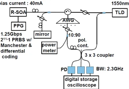
Reflection tolerant coherent WDM-PON

(1)

Upstream Channel Simulation

The system efficiency was measured for the proposed self-homodyne and differential coding receiver in a back to back configuration. We considered the experimental set-up outlined in figure 3.1 [1] and the first two BER curves “coherent with and without reflections” in Figure 4 b [1] as reference to validate the simulator. In our simulations, the tool noise parameters were calibrated in order to meet those results in absence of reflections.

(2)

The performances were tested for two different configurations:

• During the first part of the project, some simulations were made without reflections to verify the better sensivity of the proposed coherent receiver.

• In the second part, reflection noise was added to observe the behavior of the system against reflections and get BER measurement.

3.1. Simulation set up in absence of reflections

In according with the considered values for experiments presented in [1], the following parameters were set:

• Power of seed light injected into RSOA,S_in−_RSOA =−22dBm • Power of reference light at the seed laser as dBm0

• RSOA gain,G =19dB

• Extinction ratio, r_ext, of 3.6dB

• RSOA equivalent noise figureNF =8dB • Bit-rate R_b =1.25 Gbps

• Received Power has been varied from P_r =−47dBm toP_r =−26dBm

by an attenuator.

We started to generate the transmitted signal with a Simulink program. Original bits are preliminary coded with a non-return-to-zero coding, then a differential coding was applied. Keeping extinction ratio fixed to 3.6 dB at optical reflective modulator, we calculated the linear amplitudes, A and B, while varying the received power P_rat OLT (see the expression reported in 2.3). An attenuator was used to set the received power from −47dBm to −26dBm; we accordingly scaled the

(3)

noise power generated by R-SOA to hold the same OSNR, calculated in paragraph 2.4. (Note that OSNR was set to 28 dB).

10 2 2 10 RSOA in dBm r S P n − + σ = σ W

The received upstream signal light and R-SOA noise, E_m(t)+E_RSOA(t), were

injected to a port of the 3 x 3 coupler and the reference light, E_ref(t), was injected to

another port. As concerned the reference power, we set the splitter ratio at OLT equal to 50%; this implies a loss of 3+1.5 = 4.5 dB. Referring at the experimental set-up outlined in Figure 3.1 the local oscillator power at the receiver is

7 . 10 5 . 1 7 . 4 5 . 4 0− − − = = lo

P dBm, where the second loss is due to 1:3 coupler ratio.

Then A_l = 2P_lo = 0.01294 W. The reference phase was chosen at random between 0 and 2 . For the reported obtained results, the phase was 2.5097π ≅0.79⋅π.

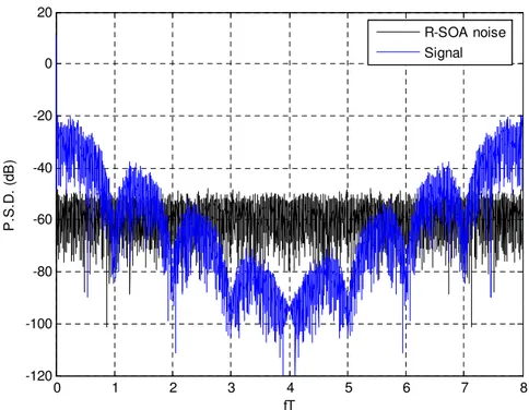
Figure 3.2 outlines the Power Spectral Density of upstream signal and noise

0 1 2 3 4 5 6 7 8 -120 -100 -80 -60 -40 -20 0 20 fT P .S .D . (d B ) R-SOA noise Signal

(4)

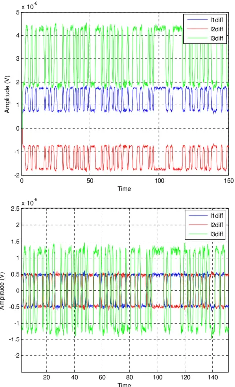
The performance was estimated using the analogic – digital conversion. To better clarify how the receiver acts on the input we reported the waveforms of the currents in various key points of the structure. For this purpose we did not introduced thermal noise and we processed the signal for a received power of P_r= -40 dBm. Figure 3.3 shows the terms i₁(t), i₂(t) and i₃(t), that are the three photo-diodes output currents. 0 50 100 150 5.2 5.3 5.4 5.5 5.6 5.7 5.8 5.9 6 6.1 6.2x 10 -5 A m p lit u d e ( V ) Time i1(t) i2(t) i3(t) Fig. 3.3 – Photocurrents

During the signal processing the photocurrent of the coupler outputs get in the differential amplifiers. Then I₁diff(t)_, ₍ ₎

2 t

Idiff _and ₍₎

3 t

Idiff pass a capacitor for DC – blocking. Currently we do not care to design an appropriate high pass filter (HPF) since the reflection has not been introduced and its aim is not cut out the crosstalk yet. Figure 3.4 (a) and (b) outlined the currents before and after the AC coupling.

(5)

0 50 100 150 -2 -1 0 1 2 3 4 5x 10 -6 A m p lit u d e ( V ) Time I1diff I2diff I3diff 20 40 60 80 100 120 140 -2 -1.5 -1 -0.5 0 0.5 1 1.5 2 2.5x 10 -6 A m p lit u d e ( V ) Time I1diff I2diff I3diff

(6)

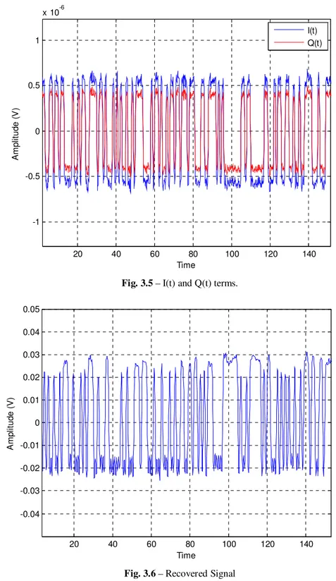
20 40 60 80 100 120 140 -1 -0.5 0 0.5 1 x 10-6 A m p lit u d e ( V ) Time I(t) Q(t)

Fig. 3.5 – I(t) and Q(t) terms.

20 40 60 80 100 120 140 -0.04 -0.03 -0.02 -0.01 0 0.01 0.02 0.03 0.04 0.05 A m p lit u d e ( V ) Time

(7)

Figure 3.5 presents I(t) and Q(t) terms calculated as linear combination of the currents from 3.4 (b). They presents terms cos( φ∆ ) and sin( φ∆ ), respectively; this implies a complete phase recovery after the differential decoding. The merit of coherent receiver is that signals recovered from I(t) and Q(t) can be added to increase the signal power. Figure 3.6 shows the final decoded signal, S(t).

3.2. Coherent receiver performance without optical reflections

In this paragraph we reported the results related to the first part of the simulation’s project. This mode of operation is intended to assess the benefits from the proposed coherent receiver respect conventional receiver with signals free from interference.

Due to delays introduced by used filters, we neglected the last five transmitted bits and the first three received for sake of precision. In order to detect the optimal sampling time the eye diagrams were plotted at different received powers.

The following figures, obtained through the MATLAB program, outline eye diagrams for P_r =−44dBm, P_r =−40dBm, P_r =−32dBm and P_r =−26dBm.

Q-factor and bit-error-rate were calculated and the obtained curves are depicted in Figure 3.11 and 3.12. Preliminary results confirmed the good sensitivity of the upstream signal and were very close to experimental results described in [1]. They were used as baseline for performance evaluation in presence of reflections induced impairments.

(8)

-1 -0.5 0 0.5 1 -0.06 -0.04 -0.02 0 0.02 0.04 0.06 Time A m p lit u d e Eye Diagram

Fig. 3.7 – Eye diagram with Pr= -44 dBm

-1 -0.5 0 0.5 1 -0.05 -0.04 -0.03 -0.02 -0.01 0 0.01 0.02 0.03 0.04 0.05 Time A m p lit u d e Eye Diagram

(9)

-1 -0.5 0 0.5 1 -0.03 -0.02 -0.01 0 0.01 0.02 0.03 0.04 Time A m p lit u d e Eye Diagram

Fig. 3.9 – Eye diagram withPr= -32 dBm

-1 -0.5 0 0.5 1 -0.03 -0.02 -0.01 0 0.01 0.02 0.03 0.04 Time A m p lit u d e Eye Diagram

(10)

-45 -40 -35 -30 -25 6 8 10 12 14 16 18 20 22 Received Power (dBm) Q F a c to r (d B ) Fig. 3.11 – Q factor -45 -40 -35 -30 -25 10-35 10-30 10-25 10-20 10-15 10-10 10-5 100 Received Power (dBm) B E R Fig. 3.12 – BER

(11)

The simulation results obtained for a received power of P_r =−40dBm were:

• Q-factor = 14.387 dB

• BER = 8.0261e-008

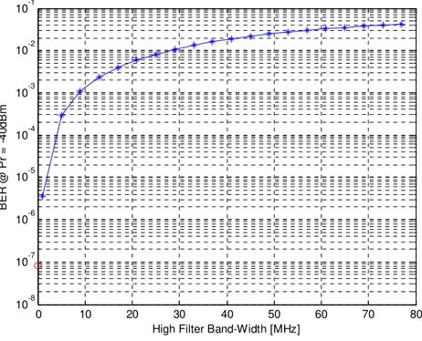
Still considering this received power, we processed the signal at the receiver by varying the high pass filter band, B_a

,

which replace the capacitor. The frequency cut-off was change from 1 to 80 MHz; it should be chosen so that it exceeds the width of the interference spectrum and it decreases the signal as little as possible. We ran simulations by using a single pole high pass filter, as described in the previous chapter. This test was made because we were using a non return-to-zero (NRZ) line coding; this kind of coding presents the most of frequencies spectrum content around the low frequencies, then a high bandwidth filter could strongly affects bit error rate measurement. As we expected, the great part of the signal was cancelled out from the filter band.

Looking at the Figure 3.13 we deduced that to obtain acceptable performances we could not use a high cut off frequency and this could become a problem when the reflection noise was added to the signal. The red circle in figure outlines the BER = 8.0261e-008 value.

To validate our results we made the same operations by scanning all possible reference phase values. From Figure 3.14 it can be possible to deduce that this value is not particularly significant, and then we concluded that this value could be neglected for our purpose of calculation. The red line in 3.14 represented the curves of Figure 3.13 obtained for φ_ref =2.5097.

(12)

0 10 20 30 40 50 60 70 80 10-8 10-7 10-6 10-5 10-4 10-3 10-2 10-1

High Filter Band-Width [MHz]

B E R @ P r = -4 0 d B m

Fig. 3.13 – BER vs High pass filter bandwidth

0 10 20 30 40 50 60 70 80 10-6 10-5 10-4 10-3 10-2 10-1

High Filter Band-Width [MHz]

B E R @ P r = -4 0 d B m

(13)

3.3 Coherent receiver performance with optical reflections

In CW-feed reflective PONs, the crosstalk generated by reflections of the seeding light produces beat noise at the Optical Terminal Line. This paragraph is related to the second part of the simulations when reflection signal was added.

For a NRZ signal, 50 % of the crosstalk noise power is confined around the zero frequency, extending on a spectral region, f∆ , determined by the shape and the line-width of the interfering signal (typically ∆f ≅MHzfor DFB lasers) As reported in the previous section of this script, it was modeled as band limited Gaussian noise. A low pass filter is used to limit the frequency band of the reflection. Its response is expressed as: a LP B f j f H π − = 2 1 1 ) ( .

(

Nc Tsim

)

/ 1 ) f ( = ⋅

∆ , where T_sim is the simulation time and N the number of samples _c

per symbol. Therefore, in a discrete domain it becomes:

a LP B f k j k H ) ( 2 1 1 ) ( ∆ π − = . a

B is the band of the filter normalized to the bit-rate R_b. Reasonably, It was taken

equal to 0.008⋅R_b, that corresponds to 10 MHz .

Conventional AC-coupled receivers are designed to work with interferences signal free and encompass a DC-block with low frequency cut-off in the KHz region, but in presence of large noise value they show bad results. Using a proper post-detection high pass filter it is possible to improve the resilience to reflections. If the cut-off frequency is chosen so that exceeds the width of the interference spectrum, the receiver could exhibit the AC-coupled performance also at high Optical Signal to Noise values. However such aggressive DC-blocking has limited effectiveness

(14)

because of the signal power spectrum. In this case the NRZ coding seems to be not particularly suitable having high power at low frequency as the noise. In fact we observed substantial eye distortions.

For the purpose of the calculation we set the reflection ratio, defined as power

of reflected seed light divided by power of upstream signal light, to r R

P P

= -10 dB.

Figure 3.15, Figure 3.16, Figure 3.17 and Figure 3.18 outline the obtained eye diagram for the specified received powers.

The bit-error-rate measurement is reported in Figure 3.19. In Figure 3.20 BER is compared with the performance measured in case of absence of reflection (BER of Figure 3.12 is now the red line).

For received power P_r =−40dBm, the following result was obtained:

• Q-factor = 5.3293 dB

• BER = 0.0324

In the eye diagrams we observed that noise affected more the mark symbol but, however, the reflections are strongly detrimental for the proposed system which not presents a tolerance to impairments induced by reflections signal and doesn’t work with acceptable performance in this way. The BER’s curve collapsed to bad value even for higher receiver powers.

We needed a solution to make more effective the post-detection high pass filtering and make the coherent AC-coupled system tolerant to reflection also at low optical signal-to-noise ratio. In the next paragraphs we proposed to re-code the transmitted signal and re-run the same simulation steps made in this first section, so as to compare the behavior

(15)

-1 -0.5 0 0.5 1 -0.08 -0.06 -0.04 -0.02 0 0.02 0.04 0.06 0.08 0.1 Time A m p lit u d e Eye Diagram

Fig. 3.15 – Eye diagram -44

-1 -0.5 0 0.5 1 -0.08 -0.06 -0.04 -0.02 0 0.02 0.04 0.06 0.08 0.1 Time A m p lit u d e Eye Diagram

(16)

Fig. 3.17 – Eye diagram -32

(17)

-45 -40 -35 -30 -25 10-1.6 10-1.5 10-1.4 10-1.3 10-1.2 Received Power (dBm) B E R Fig. 3.19 – BER -45 -40 -35 -30 -25 10-35 10-30 10-25 10-20 10-15 10-10 10-5 100 Received Power (dBm) B E R Fig. 3.20 – BER

(18)

3.4. Electrical filtering and line coding techniques to mitigate the reflection penalty A solution is proposed to increase the system tolerance to in-band reflection. The enhancement is achieved by a combined use of a suitable line coding and ad-hoc post-detection electrical filtering. In light of what we have obtained with previous simulations, we can say that the High Pass Filtering approach is resulted really effective when related with a proper encoding such is the data stream is DC balanced, e.g. Manchester coding or even 8B/10B coding.

We tried to do the same simulation steps of the previous section, by introducing a Manchester code rather than a NRZ code.

After a briefly introduction about the characteristics of the two considered line coding, the obtained results of the system simulation are reported.

3.4.1. Line Codes

A digital signal is a discontinuous signal that changes from one state to another in discrete steps. A popular form of digital modulation is binary, or two levels, digital modulation. In binary modulation the optical signal is switched from a low-power level (usually off) to a high-power level. Line coding is the process of arranging symbols that represent binary data in a particular pattern for transmission.

The most common types of line coding used in fiber optic communications include non-return-to-zero and Manchester already considered in our simulations.

As said above, we used a NRZ code for the first simulation runs. From the obtained result we inferred that the use of a different encoding is strictly necessary to make acceptable system performance even in presence of crosstalk due to reflections; and it seems to be more interesting because of the high pass filter. By using the Manchester coding is possible to reduce the signal power in the low frequency range, and then the high pass filter can have a wider band for a better decreasing of reflected noise without to be aggressive on the signal power, too.

(19)

Here the main differences between the two line coding are reported:

• Non return to zero code

NRZ code represents binary 1s and 0s by two different light levels that are constant during bit duration. The presence of a high-light level in the bit duration represents a binary 1, while a low-light level represents a binary 0. NRZ codes make the most efficient use of system bandwidth. However, loss of timing may result if long strings of 1s and 0s are present causing a lack of level transitions. It contains a DC component too.

It is generally used to code digital data from/to terminal device.

1 0 1 0 1 1 1 0 0 1 0 1 0 1 1 1 0 0

Unipolar NRZ code

1 0 1 0 1 1 1 0 0 1 0 1 0 1 1 1 0 0 1 0 1 0 1 1 1 0 0 1 0 1 0 1 1 1 0 0

Unipolar NRZ code

Fig. 3.21 – Non-return-to-zero code

• Manchester code

Manchester code incorporates a transition into each bit period to maintain timing information. We considered the convention generally followed by transmission standards that a high-to-low light level transition occurring in the middle of the bit duration represents a binary 0; a low-to-high light level transition occurring in the middle of the bit duration represents a binary 1. This code has the advantages of embedding timing information (clock) within the transmitted bits

(20)

1 0 1 0 1 1 1 0 0 1 0 1 0 1 1 1 0 0 Manchester code 1 0 1 0 1 1 1 0 0 1 0 1 0 1 1 1 0 0 1 0 1 0 1 1 1 0 0 1 0 1 0 1 1 1 0 0 Manchester code

Figure 3.22 – Manchester code

Although this allows the signal to be self-clocking, it doubles the bandwidth requirement compared to NRZ coding schemes; however the content of the power density is greater at high frequencies and the DC component of the encoded signal is not dependent on the data and therefore carries no information, allowing the signal to be conveyed conveniently by media which usually do not use a DC component.

Therefore the next step was to simulate the receiver when the transmitted random bit stream is differentially encoded and Manchester encoded. Through the use of a MATLAB program it was possible plot the Figure 3.23 in which we can note the differences between signal Power Spectral Density (PSD in linear scale) obtained with the two encodings. In the Figure 3.24 is highlighted how the HPF works by plotting PSD in decibel scale. Non-return-to-zero coded signal is plotted in blue, Manchester coded signal in black. Obviously, because of power spectrum characteristics, the HPF has more effect with a Manchester coding.

(21)

0 1 2 3 4 5 6 7 8 0 0.02 0.04 0.06 0.08 0.1 0.12 0.14 0.16 0.18 0.2 fT P .S .D NRZ code Manchester code

Fig. 3.23 – NRZ and Manchester coding PSD

0 1 2 3 4 5 6 7 8 -100 -90 -80 -70 -60 -50 -40 -30 -20 -10 0 10 fT P .S .D

(22)

3.4.2. Manchester coded signal generation

For upstream signal simulation, we followed the same model presented in

paragraph 2.3., that was:

) cos( ) ( ) ( ₀ _s k k m t A a p t kT B t E  ω +φ      +       − ⋅ =

∑

,

T is the symbol time, p(t)is an ideal rectangular pulse with unitary amplitude

and length T, while, this time, a_k is the bits sequence preliminary differential coded

then Manchester coded. As before to recreate the digital logic gate XNOR the output stream of Differential Encoder block was subtracted to 1. To have a DC-balanced data stream we need to map the symbol set from {0,1} to {-1,1} To this purpose, we multiplied the data by -2 and then a constant equal to 1 was added. To have the mid-bit transition for data direction indication, a Pulse Generator block was introduced. It generates square wave pulses at regular intervals; we set the pulse amplitude to 2, with unitary period, duty cycle to 50 percent (specified as the percentage of the pulse period that the signal is on) and the phase delay to zero. Making the generated clock time on 1 and -1 levels a further subtraction was performed between the wave pulse and the constant 1.

The two obtained streams were multiplied and the product was filtered by a Gaussian FIR filter to shape the pulses. The block expects the input signal to be

up-sampled, so that the input samples per symbol parameter, N , was set to 8. This time c

BT was set to 2 because the data rate is double than NRZ coded stream. One more time the constant B was added to consider the extinction ratio; to obtain the linear amplitude of the upstream signal we performed substantially the same operations

reported in the paragraph 2.3. Here the m(t) mean square value., E_m2(t) =P_r, changed respect to before.

(23)

[

]

     = ⋅ + + ⋅ = + r P AB B A B B A 2 0 2 1 10 2 2 10 6 . 3

From the first relation it was obtained (1010 1)

6 . 3 − ⋅ = B

A ; from the second

        ⋅ − +         = 10 6 . 3 2 10 6 . 3 10 2 2 10 2P_r B .

In the Figure 3.25 the Simulink scheme to generate the upstream signal implementing a Manchester coding is depicted. Then the signal was sampled and exported as a vector to MATLAB ready to be processed in the same programs implemented for the simulations in paragraph 3.2. and 3.3.

(24)

3.5. Simulation without optical reflections in presence of filtering and line coding Experimental set-up and parameters set were the same used in paragraph 3.1. included the tool noise parameters. So we reported the results related to test the coherent receiver performance by using received signals free from interference. The optimal sampling time were inferred by the eye diagrams. In the Figures 3.26 and 3.27 diagrams for P_r =−40 dBm and P_r =−26 dBm, respectively, were outlined. From

their observation we immediately noticed an improvement in performance, then confirmed by the curves obtained from the calculation of Q-factor and bit error rate (Figure 3.28 and 3.29).

To understand this improvement we have designed the Power Spectral Density of NRZ coded signal and Manchester coded signal with that of thermal noise. The PSD plotted in linear scale highlights that the useful power is greater in the second case and concentrated on a main lobe double respect to that of NRZ code, while the thermal noise is the same in both cases, as it should be. (Figure3.30 and 3.31) Since

the electrical band of our receiver is 2.3 GHz = 1.84 R , as the most realistic _b

receivers, the optical signal-to-noise ratio is higher for the Manchester coded signal. If

we had used an electric filter with bandwidth equal to the bit-rate, R_b, we always

obtained better performance of the second case respect to the first, although reduced compared to our receiver. This is because NRZ coded signal presents a high DC power component while it is not present in Manchester coded signal. After DC-block due to the AC coupling this component were cancelled out causing a worse effect on BER in NRZ case.

(25)

-1 -0.5 0 0.5 1 -0.15 -0.1 -0.05 0 0.05 0.1 Time A m p lit u d e Eye Diagram

Fig. 3.26 – Eye diagram with P_r =-40 dBm.

(26)

-45 -40 -35 -30 -25 17 18 19 20 21 22 23 24 25 26 Received Power (dBm) Q F a c to r (d B ) Fig. 3.28 – Q-factor -45 -40 -35 -30 -25 10-80 10-70 10-60 10-50 10-40 10-30 10-20 10-10 Received Power (dBm) B E R Fig. 3.29 – BER

(27)

0 1 2 3 4 5 6 7 8 0 0.01 0.02 0.03 0.04 0.05 0.06 0.07 0.08 0.09 0.1 P .S .D . fT signal thermal noise

Fig. 3.30 – PSD of NRZ coded signal with thermal noise

0 1 2 3 4 5 6 7 8 0 0.02 0.04 0.06 0.08 0.1 0.12 0.14 0.16 0.18 P .S .D . fT signal thermal noise

(28)

For the received power P_r =−40dBm, the following result was obtained:

• Q-factor = 22.3 dB • BER = 4.0644 e-039

To validate what has been stated above, we calculated the BER also using an electrical filtering with bandwidth equal to the bit-rate. We obtained:

• Q-factor = 19.708 dB • BER = 2.0366 e-022

Next step regards the signal processing by varying the high pass filter band,

a

B

.

As we expected we note a more limited worsening of BER for the considered frequency cut-off range. Looking at the Figure 3.32 we deduced that a suitable design of the HPF combined to a DC-balancing line code could enhance the system even in presence of reflections. The red circle in figure is BER = 4.0644 e-039 (obtained by carving just DC component). Scanning all possible reference phase values we found a not substantial bit-error-rate variation so that we can neglect its particular value in our simulations. The red line in 3.33 represented the curves of Figure 3.32 obtained for

2.5097 =

(29)

0 10 20 30 40 50 60 70 80 90 100 10-39 10-38 10-37 10-36 10-35

Banda del filtro Passa Alto [MHz]

B E R c a lc o la ta c o n P r = -4 0 d B m

Fig. 3.32 – BER vs HPF frequencies cut-off

0 10 20 30 40 50 60 70 80 90 100 10-50 10-40 10-30 10-20 10-10

Banda del filtro Passa Alto [MHz]

B E R c a lc o la ta c o n P r = -4 0 d B m

(30)

3.6. Simulation with optical reflections in presence of filtering and line coding The reflection signal was added as Gaussian noise in a band of 0.008⋅R_b = 10

MHz . The reflection ratio between reflection power and received power, r R

P P

, was set

to -10 dB. We got optimal results as concerned the reflection tolerance. Surely the crosstalk due to reflections introduced a penalty in the performance evaluation but it is very impressive in a positive way how, even in presence of potentially destructive optical signal to noise ratio, the performance was greatly improved. Indeed further

lowering the optical signal to noise ratio to get r R

P P

= 0 dB we obtained very close

curves and acceptable bit-error-rate value.

This has demonstrated the potential strong tolerance to the reflections of the system, pointing out two key aspects to consider: the high pass filter design and the use of line code.

Also the spectral shape of the beating noise depends on the line-width of the seeding laser. In order to optimize the system performance, the HPF should be therefore designed according to the specification of the laser and the used line code. Optimization is expected to be less critical at increasing data-rates: in fact while the beating noise spectrum is confined manly around the DC at increasing data-rates, the low frequency carving operated by the Manchester, or also by the 8B/10B code, extends over a wider range. We thus expect that the effectiveness of the proposed solution can be easily extended to bidirectional PON system operated at higher data rates. The following figures outline eye diagrams for P_r =−44dBm, P_r =−40dBm,

32 − = r

P dBm and P_r =−26dBm obtained adding crosstalk with the first reflection

ratio. The distortion observed at lower level of the eye was due to the HPF cut-off frequency. If it was set higher, more distortion was observed; however the cross point and aperture point are not affected in this sense.

(31)

-1 -0.5 0 0.5 1 -0.2 -0.15 -0.1 -0.05 0 0.05 0.1 0.15 Time A m p lit u d e Eye Diagram

Fig. 4.34 – Eye diagram P_r =-44 dBm.

(32)

Fig. 3.36 – Eye diagram P_r =-32 dBm.

(33)

-45 -40 -35 -30 -25 10-80 10-70 10-60 10-50 10-40 10-30 10-20 10-10 Received Power (dBm) B E R

Fig. 3.38– BER without and with reflections.

-45 -40 -35 -30 -25 10-80 10-70 10-60 10-50 10-40 10-30 10-20 10-10 Received Power (dBm) B E R

Fig. 3.39 –BER comparison obtained with r R P P =-10 dBm and r R P P =0;

(34)

In order to demonstrate the tolerant of the proposed system to crosstalk we set the high pass filter frequencies cut-off to 80 MHz. Figures 3.38 and 3.39 exhibits the obtained performances. The red line represents the bit-error-rate curves without reflections, the blue line is obtained with a reflection ratio of -10 dB and the green line is obtained with a reflection ratio of 0 dB.

A last simulation was run to observe the behavior of the system by varying the power of the reference light. Until now we guessed a splitter ratio at OLT of about 50 percent. We tried to change this value from 5% to 50%; since the amplitude of detected currents is also proportional to reference light, we expected a worsening of the performance given by a lowering of the reference power signal. The curves in

figure 3.40 and 3.41 were obtained for a P_r= - 40 dBm and a reflection ratio of -10 dB

and 0 dB, respectively. The reference phase was keeping fixed to φ_ref =2.5097.

Obviously the lower curve is related to 1:2 splitter ratio.

0 10 20 30 40 50 60 70 80 90 100 10-40 10-35 10-30 10-25 10-20 10-15 10-10 10-5

BER With Reflected ratio -10 dB vs HP band and Reference light power

High Filter Band [MHz]

B E R @ P r = -4 0 d B m

(35)

0 20 40 60 80 100 120 10-35 10-30 10-25 10-20 10-15 10-10 10-5 100

BER With Reflected ratio 0 dB vs HP band and Reference light power

High Filter Band [MHz]

B E R @ P r = -4 0 d B m