A Pathway to EMU: the SCORPIO Project

(1)

Universit`

a degli studi di Catania

Facolt`a di scienze matematiche fisiche e naturali

Dottorato di ricerca in Fisica

FRANCESCO CAVALLARO

A Pathway to EMU:

The SCORPIO Project

PhD Thesis

COORDINATOR: Prof. V. Bellini SUPERVISOR: Prof. F. Leone TUTORS: Dr. C. Trigilio XXIX Ciclo

(2)

List of Tables

1.1 _{Physical parameters of H ii regions (Kurtz, 2005). . . 18}

2.1 Instrumental parameters of SKA1. The rms is calculated for

a 1-hour observation, considering the whole band. . . 31

3.1 Age, metallicity, radial metallicity gradient, initial mass

func-tion and star formafunc-tion rate of the stellar components. . . 43

3.2 Typical OB stars parameters from Panagia (1973). ZAMS is

the zero main sequence, V, III and I are the luminosity class

of dwarf, giant and hypergiant. . . 47

3.3 Number of total stars Ntot and number of MCP at every

spec-tral types in the Catalano & Leone (1994) sample. . . 49

3.4 Expected number of RS CVn binaries detected per square

de-gree on the Galactic Plane at 1, 5, and 50 µJy, based on the

work described in this chapter. . . 53

3.5 Expected number of OB stars detection per square degree at

different Galactic Longitude, fixing the Galactic Latitude to −1 < b < 1 based on the work described in this chapter at 1,

5 and 50 µJy. . . 53

3.6 Expected number of MCP stars detection per square degree

at different Galactic Longitude, fixing the Galactic Latitude to −1 < b < 1 based on the work described in this chapter at

1, 5 and 50 µJy. . . 53

3.7 Expected number of M stars detection per square degree based

on the work described in this chapter at 1, 5 and 50 µJy. . . . 54

4.1 Observing parameters for the 6km array (except for the W

band, for which it is assumed the H214 configuration without

the CA06 antenna.) (Stevens et al., 2016). . . 60

4.2 Observations log. . . 60

(5)

LIST OF TABLES 4

4.3 Sub-band frequency and primary beam radii at 5 percent of

the peak. . . 69

4.4 Number of matched sources. NA stands for not applicable due

to the overcrowding of the catalogue. . . 73

5.1 Criteria to exclude models based on their higher BIC in respect

with other models as in Kass et Raftery (1995). . . 89

5.2 BIC for every model considered for the SCORPIO survey.

Ev-ery Gaussians needs 3 parameters while the skewed Gaussians

need 4 ones. . . 90

5.3 BIC for every model considered for the ATLAS survey.

Ev-ery Gaussians needs 3 parameters while the skewed Gaussians

need 4 ones. . . 90

6.1 Product of the primary beam FWHM and frequency at every

SCORPIO sub-band, using the recent measurements of the primary beam for the new 16-cm CABB receiver (d) and the

(6)

List of Figures

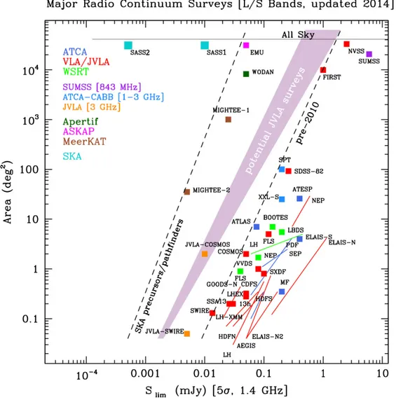
1.1 Area plotted against sensitivity of the most important surveys

pre-2010 compared to the future ones (Norris et al., 2015). The plot shows that we will explore an unexplored survey

param-eter space, that will, for sure, produce a lot of new results. . . 11

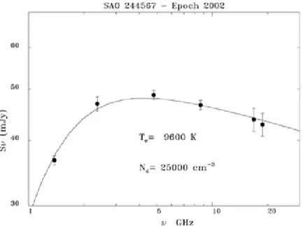
1.2 Spectrum of the SAO 244567 nebula (Umana et al., 2008). It

presents the typical thermal bremsstrahlung spectrum. . . 14

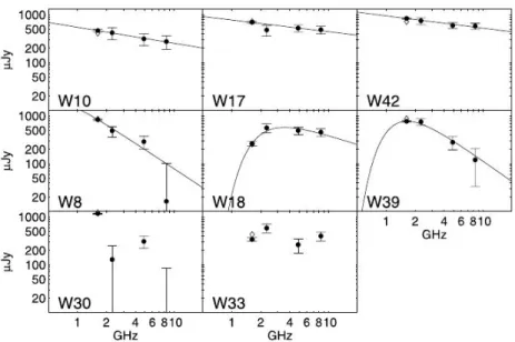
1.3 Spectra of four galaxies. NGC 1275 and 3C 454.3 (first and

last panels) present a superposition of different emission mech-anism, while 3C 123 and 3C 48 (second and third panels) present a synchrotron spectrum (Verschuur, Kellermann, &

van Brunt, 1974) . . . 14

1.4 Example of an Fanaroff-Riley type I (FR I) galaxy. This is a

radio map of the Virgo cluster elliptical galaxy M84 (Laing &

Bridle, 1987). . . 16

1.5 Example of an Fanaroff-Riley type II (FR II) galaxy. This is

a map of the quasar 3C 175, as observed with the VLA at 4.9

GHz (Bridle et al., 1994) . . . 17

1.6 Superposition of 8-µm image and 6-cm contours of MGE 031.7290+00.6993

(Ingallinera et al., 2016). . . 19

1.7 Image of Cassiopeia A in radio, taken with the VLA in the

NVSS survey. . . 20

1.8 Radio spectra of some supernovae remnant older than 11 years

(Parra et al., 2007). . . 20

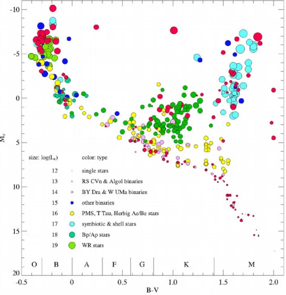
1.9 HR diagram of all known radio stars as in the G¨udel (2002)

440 stars sample. . . 21

1.10 Radio images of Algol at three different orbital phases. Notice the radio emission localised near the evolved star, pointing towards the main sequence star (Peterson et al., 2010). The

cross represents the position error. . . 24

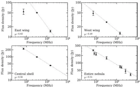
1.11 Spectrum of the W50 nebulae components, surrounding the

SS433 microquasar (Miller-Jones et al., 2007) . . . 25

(7)

LIST OF FIGURES 6 1.12 Spectrum of several planetary nebulae (Gruenwald & Aleman,

2007). . . 26

2.1 The ASKAP site from captured from an helicopter. . . 32

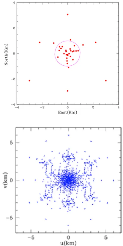
2.2 ASKAP antennae configuration and corresponding uv plane

in a 12 minute observation. . . 33

2.3 Phased Array Feed mounted on an ASKAP antenna. . . 34

2.4 First image of ASKAP-12 at 36 beams. Notice the huge FOV. 35

2.5 Expected redshift distribution of the EMU sources. RQQ

are radio quiet quasars, FR1 and FR2 are the Fanaroff-Riley

galaxies type 1 and 2. . . 37

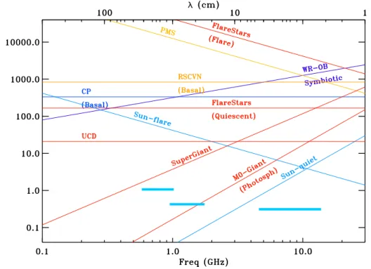
2.6 Average spectrum of common radiostars classes. The WR-OB

and giant stars are assumed to be at 1 kpc, the MCP at 0.5 kpc, the RS CVn, flare stars and sun-like stars at 10 pc and the Ultra Cool Dwarf (UCD) at 20 pc. The pale blue horizontal lines represent the SKA-1 1 σ for an hour of observation at

the three different bands. . . 38

2.7 Expected flux of common radio stars classes versus their

dis-tance from the Earth at 5 GHz. The pale blue horizontal line

represents the SKA1 1σ 1-hour observation. . . 39

3.1 Components of our Galaxy . . . 43

3.2 log N -log S distribution for a galactic latitude −1 < b < 1 at

different galactic longitude. The black line is at 50 µJy, the EMU sensitivity, while the blue one is at 1 µJy, the SKA-1

25-hours sensitivity. . . 46

3.3 Density of OB stars with a flux greater than 1 µJy for −1 <

b < 1, 1 < b < 3 and 3 < b < 23 with respect to galactic

longitude. . . 46

3.4 log N -log S distribution for a galactic latitude −1 < b < 1 at

different galactic longitude. The black line is at 50 µJy, the EMU sensitivity, while the blue one is at 1 µJy, the 25-hours

SKA-1 sensitivity. . . 49

3.5 Density of MCP stars with a flux greater than 1 µJy for −1 <

b < 1, 1 < b < 3 and 3 < b < 23 with respect to galactic

longitude. . . 50

3.6 log N -log S distribution at different galactic latitude and

lon-gitude of flare stars. The yellow line is at 1 µJy, the 25-hours

SKA-1 sensitivity. . . 51

3.7 Number of RS CVn in the Eker et al. (2008) catalogue at each

(8)

4.1 Four of the six ATCA dishes . . . 59

4.2 uv plane of a pointing of the SCORPIO observations at 3.124

GHz resulting from the sum of all the observing intervals. No-tice the central part of the uv plane, filled by the short baseline

observations. . . 61

4.3 pgflag user interface. In abscissa the channel number

(in-creasing frequency toward left), in ordinate the scan numbers. 64

4.4 Spectra of the phase calibrator 1714-397 for all the baselines

after the baselines and flux calibrations. In abscissa the fre-quency, in ordinate the amplitude, 0-3.5 scale in the a subplot, 0-4.5 in the b one. Notice the flagged 4-5 baseline on the

ex-tended configuration plot. . . 66

4.5 Map of the complex calibrator. It is shown how the field is

confused by an extended emission around the calibrator that causes the problem in the shortest baselines and by two bright sources. The calibrator is 2.1 Jy bright, the other two source are 370 and 237 mJy without the primary beam correction,

that is not known at that angular distance from the centre. . . 67

4.6 A particularly bright and extended source before and after the

self calibration. Notice the reduction of bright lines artefacts

and of the rms, from 210 µJy to 140 µJy. . . 70

4.7 Final map of SCORPIO . . . 71

4.8 SCORPIO pilot field showing the primary beam at the lowest

and highest frequency. . . 73

5.1 Flowchart for the flux extraction algorithm . . . 76

5.2 Spectrum of SCORPIO1 243. In green the straight linear fit

while in red the line of the fit after the application of the

turnover algorithm is showed. . . 77

5.3 Spectral index extraction algorithm flowchart. . . 79

5.4 Map of one of the double sources, SCORPIO1 334. The

pur-ple contour represents the gaussian fit made by the described

algorithm. To fit this source the script used 4 gaussians. . . . 81

5.5 Spectrum of SCORPIO1 334. The straight green line

repre-sents the linear fit. The points result from the sum of the

value of each of the 4 gaussian at each frequency. . . 82

5.6 Grey scale of the 16 SCORPIO sources with a MGPS-2 match.

The black ellipse embedding the sources is the Molonglo beam. 83

5.7 Continued from the previous figure. . . 84

5.8 Spectra of the 16 sources selected among the 43 sources that

(9)

LIST OF FIGURES 8

5.9 Continued from the previous figure. . . 86

5.10 Spectral indices against signal-to-noise ratio in the simulation. All the sources have been built to have a flat SED, but the spectral indices are not accurate enough below 40σ (indicated

by the red line). . . 87

5.11 The median on the spectral indices error against

signal-to-noise ratio in SCORPIO. . . 88

5.12 Spectral index distribution of the SCORPIO survey using a 0.25 wide bin in blu straight line, modeled using 3 Gaussians (red dashed line). In black dash-point line the three Gaussian

components of the final model. . . 88

5.13 Number of sources per square degree in a 0.25 wide bin his-togram for the ATLAS survey, modelled as a skewed Gaussian

(red dashed line). . . 91

5.14 SCORPIO spectral index distribution modelled as a sum of

the ATLAS model and a Gaussian. . . 93

5.15 Difference between the SCORPIO and the ATLAS spectral

indices histogram. . . 94

6.1 First iteration map of the whole field, using only the extended

configuration observations, before the primary beam correction. 96

6.2 Region around the s17 in the first iteration map. Notice the

artefacts and the missing flux. . . 97

6.3 Map of the SCORPIO Galactic Plane done using mosmem. . . . 99

6.4 An extended source of the SCORPIO field, deconvolved using

the CLEAN and the MEM algorithm. The CLEANed source is badly imaged because of how the CLEAN algorithm works, assuming that sources are made of a collection of point sources.100

6.5 Region around the s17 adding up the short baselines from the

compact configuration. Notice the differences with Fig. 6.2. . . 101

6.6 Stokes Q map of the SCORPIO field at the 4th sub-band. . . . 103

6.7 Stokes V map of the SCORPIO field. . . 103

6.8 The rms as a function of the Galactic latitude for Stokes I

(dashed line) and Stokes V (solid line). For each pixel of the map the rms has been averaged over 0.3 deg in longitude. . . . 104

6.9 Flowchart of the CAESAR algorithm . . . 105

6.10 Four sources from the Anderson et al. (2014) catalogue. The “K” regions denote a confirmed H ii region while the “C” ones denote a candidate. . . 107

(10)

6.11 Two sources from the Anderson et al. (2014) catalogue clas-sified as radio quiet. As it is shown, they are detected in

SCORPIO. . . 108

6.12 The source SCORPIO1 534 and its candidate H ii region en-velope. . . 108

6.13 The source SCORPIO1 12, ζ1 Sco. . . 109

6.14 The source SCORPIO1 118. . . 110

6.19 The sources SCORPIO1 406 and SCORPIO1 350. . . 113

6.20 HD151965, detected in SCORPIO. The red line inside is the 3σ contour of the Stokes V emission. . . 114

6.21 Final map of SCORPIO with a zoom on several sources. From the bottom left, going clockwise: S17, a star forming H ii region; a candidate H ii region; several H ii regions candidates; a Supernovae Remnant; a huge H ii region; a radio galaxy; several sources comprising a couple of sources matching with stars in open cluster; WR 79, a Wolf-Rayet star and ζ1 _Scorpii, a blue hypergiant in the Scorpio constellation. . . 115

(11)

Chapter 1 Introduction

We are entering a golden age for radio astronomy. There are several new interferometers upcoming, whose characteristics, in terms of sensitivity, fre-quency coverage, angular and temporal resolution, field of view etc., will permit unprecedented deep observations. The most outstanding ones among them will be the Square Kilometre Array (SKA, Carilli & Rawlings 2004) and its precursors, such as the Australian SKA Pathfinder (ASKAP) and MeerKAT. Several surveys will be carried out, in continuum and spectral line. In particular, in continuum, the scientific interest is both for galactic and extragalactic science, for which surveys at low or high galactic latitude are planned, such as the Evolutionary Map of the Universe (EMU; Norris et al. 2011), to be carried out with ASKAP, the MeerKAT International Gi-gaHertz Tiered extra-galactic Exploration Survey (MIGHTEE, Jarvis 2015) and the MeerKAT High Frequency Galactic Plane Survey (Meer-GAL), both to be carried out with MeerKAT.

Many radio surveys have been carried out in the past years. In continuum the NRAO Very Large Array (VLA) Sky Survey (NVSS; Condon et al. 1998) is the largest existing survey. Other important surveys are the Multi-Array Galactic Plane Imaging Survey (MAGPIS; Becker, White, & Helfand 2006), the Co-Ordinated Radio ’N’ Infrared Survey for High-mass star formation (CORNISH; Purcell & Hoare 2010), the Hi, OH, Recombination line survey of the Milky Way (THOR; Bihr et al. 2016). In the following, we briefly discuss NVSS, the largest and most important existing survey.

NVSS was carried out with the Very Large Array between 1993 and 1996 in compact D configuration at 1.4 GHz. It covered ∼ 10.3 sr of sky with

J2000 δ > −40◦ in 217 466 pointings. It produced a catalogue of more

than 2 million sources, with an angular resolution of 45′′ and a rms of 0.45

mJy beam−1 (Condon et al., 1998). The EMU survey will cover a sky area

comparable to NVSS, but it will be 45 times more sensitive and with a better 10

(12)

Figure 1.1: Area plotted against sensitivity of the most important surveys pre-2010 compared to the future ones (Norris et al., 2015). The plot shows that we will explore an unexplored survey parameter space, that will, for sure, produce a lot of new results.

(13)

CHAPTER 1. INTRODUCTION 12 angular resolution. Considering also the difference in the uv coverage, EMU will be also more sensitive to extended structures. In Fig. 1.1 (Norris et al., 2015) we report the area of the surveys plotted against their sensitivity. Thanks to the new telescopes we should cross the “pre-2010 line” and have larger and more sensitive surveys. Details on what we could expect from EMU are discussed in the Sec 2.3.

The main focus of this thesis is on radio stars and the science that can be carried out with the new radio interferometers. Even if, in general, stars emit in radio a small fraction of their luminosity, at these wavelengths it is possible to trace different phenomena that is not possible to study by other means, e.g. the physics of their magnetospheres, the interaction with the ISM in the first and in late phases of their lives, etc. Furthermore the Galaxy is optically thin in radio, then we can observe stars in the GP that we could not observe in the optical frequencies. Unfortunately, due the faintness of stars in radio, the number of currently known radio stars is limited to a small sample.

1.1 Radio sources

One of the main goal of this work is the characterisation of different kind of radio sources. The flux density of a radio source can be generically expressed as Hjellming (1988): Sν = TBθ′′1θ ′′ 2 1960λcm Jy (1.1)

where TBis the brightness temperature, θ′′1 and θ

′′

2 are the angular dimension

of the source in arcsec and λcm is the wavelength at which we observe in cm.

This means that a source must have either high angular dimension or high brightness temperature to be detected. For thermal emission we usually have a extended source with a low brightness temperature, while for non-thermal emission it is the opposite.

In the next sections we will show the main emission mechanism in the radio wavelength and we will give an overview of the most common source classes.

1.1.1 Emission mechanism

One way to discriminate sources is to study their emission mechanism. Know-ing what makes a source emit in radio can unveil its physics and exclude that it is part of a particular class. The main responsible of the radio emission in

(14)

continuum are the bremsstrahlung and the synchrotron. The bremsstrahlung emission is caused by the coulombian interaction between a free electron and a nucleus. If the plasma is in thermodynamical equilibrium, the emission mechanism is called thermal breamsstrahlung. Synchrotron is a non-thermal mechanism, where the emission is caused by the interaction between

ultra-relativistic electrons (γ > 10, where γ = (1 − v2_/c2₎−12 _{is the Lorentz factor}

and v is the speed of the electrons) with a non-thermal energy distribution

(usually a power law N (E) = N0E−δ) and a magnetic field. If the electrons

are non-relativistic this mechanism is called cyclotron (γ < 1) and it is called gyro-synchrotron for 1 < γ < 10.

One way to discriminate between different emission mechanism is to study the source Spectral Index Distribution (SED). A parameter that characterises the SED in the radio wavelengths is the spectral index α, defined as S (ν) = S0



ν ν0

α

, where S (ν) is the flux density of the source at a given frequency

ν and S0 is the flux density at the frequency ν0. The spectral index can

change with the frequency, but both synchrotron and bremsstrahlung lose this dependence in the two limits τ ≫ 1 and τ ≪ 1, where τ is the optical depth of the source. In particular, in case of a homogeneous source of thermal bremsstrahlung we have α = 2 for τ ≫ 1 while, for τ ≪ 1, it is α = −0.1. If the density is not constant, the spectral index changes. When the density

varies as r−2, as in the case of symmetrical spherical wind from hot stars,

the spectral index is α = 0.6 (Panagia & Felli, 1975).

In the case of a homogeneous source of synchrotron we have α = 2.5 for τ ≫ 1 and, for τ ≪ 1, it depends on the spectral index δ of the energy distribution of the relativistic electrons, giving us information on this physical

parameter. In particular α = δ−1₂ so, for typical values of δ, it ranges between

−1 and −0.5 (Burke & Graham-Smith, 2014).

The frequency at which a source has an optical depth τ = 1 is the turnover frequency. Measuring the turnover frequency can allow us to constrain ad-ditional physical parameters, such as magnetic field intensity or electronic density. In Fig. 1.2 and 1.3 we show a typical spectrum of a bremsstrahlung emitting source and a syncrotron emitting one.

1.1.2 Extra-galactic sources

With the expression “extra-galactic sources” we intend all the sources exter-nal to our Galaxy. Generally speaking, these sources are far galaxies. The most luminous class of extra-galactic radio sources are the Radio Galaxies, distant Radio-Loud Quasars and Blazars. Their radio emission originates from the processes occurring in their nuclei, hosting a supermassive black

(15)

CHAPTER 1. INTRODUCTION 14

Figure 1.2: Spectrum of the SAO 244567 nebula (Umana et al., 2008). It presents the typical thermal bremsstrahlung spectrum.

Figure 1.3: Spectra of four galaxies. NGC 1275 and 3C 454.3 (first and last panels) present a superposition of different emission mechanism, while 3C 123 and 3C 48 (second and third panels) present a synchrotron spectrum (Verschuur, Kellermann, & van Brunt, 1974)

(16)

hole. For this reason they are called Active Galactic Nuclei (AGN).

AGNs produce high luminosity in a compact volume, with processes dif-ferent from the star nuclear fusion. The gravitational energy released by cold gas accreting onto the central supermassive Black Hole (SMBH) is converted in electromagnetic radiation and represent the emission source of the AGN. The SMBH loses angular moment because of viscous processes in the accre-tion disc, resulting also in high soft X-ray (. 10 keV) luminosity. Evidence of hard X-ray (& 10 keV) emission is sometimes found toward the SMBH. There are emission lines in the optical and in the UV originating from the rapidly moving gas in the gravitational potential that are usually obscured by the cold matter torus rotating in a larger orbit around the SMBH. Along the rotation axis of the SMBH, matter is ejected in plasma jets that show radio emission. The most powerful radio sources are generally hosted in elliptical galaxies (Urry & Padovani, 1995).

Radio galaxies consist of an elliptical or spiral galaxy containing the AGN, and two spatially symmetric lobes. These lobes are formed by the ejected AGN plasma and are confined by the magnetic field and deposited in the intergalactic medium. They contain ultra relativistic electrons accelerated

in a magnetic field of the order of 10−5 G. The spectral index α is usually

around −0.8, where S (ν) ∝ να _{(Burke & Graham-Smith, 2014). Galaxies}

with the jet beamed towards us result in a compact observed object with a really high luminosity (it could be 3 orders of magnitude brighter than an equivalent not beamed source). In the more compact AGN the radio emission can be optically thick, resulting in a flatter spectrum. They are historically divided into 2 categories, Fanaroff-Riley of type 1 (FR I) and type 2 (FR II) (Fanaroff & Riley, 1974). FR I galaxies are brighter near the central body and become fainter the as one approaches the outer extremities of the lobes (see Fig. 1.4), while FR II galaxies have their brightest point at the edge of the jets, in the region where they collide with intergalactic medium (see Fig. 1.5).

The Gigahertz Peaked Spectrum (GPS) and Compact Steep Spectrum (CSS) are two classes of compact extra-galactic objects, about 1 kpc in size the first, some tens the latter. They can be young radio galaxies or “frus-trated” ones, that means contained into a particularly dense intergalactic medium that limits their espansion and dimension (Randall et al. 2011; Fanti 2009). Their name is due to the particular shape of their spectra. CSS have a steep spectrum (α ≤ −0.5), while the GPS spectra have a peak around 1 ∼ 10GHz, their turnover is caused by the synchrotron self-absorption. Both of them are usually unresolved (they are resolved using VLBI methods) be-cause of their small dimensions.

(17)

Figure 1.4: Example of an Fanaroff-Riley type I (FR I) galaxy. This is a radio map of the Virgo cluster elliptical galaxy M84 (Laing & Bridle, 1987).

(18)

Figure 1.5: Example of an Fanaroff-Riley type II (FR II) galaxy. This is a map of the quasar 3C 175, as observed with the VLA at 4.9 GHz (Bridle et al., 1994)

relativistic cosmic rays diffused in the galaxy that interact with its magnetic field. The emission is correlated with the star formation rate. Galaxies with a higher than average star formation rate are called Star Forming Galaxies (SFG). Star Burst Galaxies (SBG) are characterised by a even higher star formation rate so, given the higher number of supernovae, their synchrotron emission is enhanced (Burke & Graham-Smith, 2014).

1.1.3 Galactic sources

The typical radio sources that we can observe within our Galaxy are: the Galaxy itself, with the diffuse radio emission, H ii regions, circumstellar envelopes of evolved stars, different type of stars. Many discrete sources in nearby galaxies can also be studied in a similar way thanks to their proximity. H II regions

The H ii regions are ionised nebulae surrounding one or more early type young stars. The linear size of the nebulae can range from 0.03 pc to 100 pc and more (see Table 1.1). Inside the nebulae there is a stationary equilibrium

(19)

Class of Size Density Ionised mass

Region (pc) (cm−3) (M⊙) Hypercompact _{. 0.03 & 10}6 _{∼ 10}−3 Ultracompact _{. 0.1} _{& 10}4 _{∼ 10}−2 Compact _{. 0.5} _{& 5 × 10}3 ∼ 1 Classical ∼ 10 ∼ 100 ∼ 105 Giant ∼ 100 ∼ 30 103 _{∼ 10}6 Supergiant > 100 ∼ 10 106 ∼ 108

Table 1.1: Physical parameters of H ii regions (Kurtz, 2005).

between the ionisation caused by the UV light from hot young stars and the recombination. The electron temperature is around 8000 ∼ 10000 K. The radio emission is caused by the thermal bremsstrahlung (free-free emission), the turnover frequency depends on the density and the temperature of the object but it is usually around 1 GHz (Burke & Graham-Smith, 2014). In Fig. 1.6 it is shown a compact H ii region. Note the 8-µm emission surrounding the radio emission, as in most of the H ii region, is explained as thermal emission arising from very small dust grains (PAH), that are located far from the central ionising source, beyond the photo dissociation region (PDR) (Deharveng et al., 2010).

Supernovae Remnants

Stars with a mass larger than 8M⊙in main sequence end their life in a

catas-trophic way: their core collapses in less than a second leaving a compact object as a neutron star or a black hole, while the energy released accel-erates the matter outward in a violent explosion in the phenomena called supernovae. Supernovae are caused also by the thermonuclear explosion of a white dwarf in a close binary system, where the companion, a giant o su-pergiant star, loses mass through the Roche lobe accreting the white dwarf until they reach the Chandrasekhar limit. These are type Ia supernovae. The matter ejected by the star, interacting with the interstellar medium, produces a shell enclosing a nebulae called supernovae remnant (SNR) (see Fig. 1.7). The radio emission of the SNR becomes dominant with respect to the optical as the nebulae evolve and it is caused by the synchrotron emis-sion of the shock-accelerated ultra-relativistic electrons. The spectral index α is usually around −0.5 (see Fig 1.8), as predicted by the Diffusive Shock Acceleration theory (Bell 1978a,b). There are SNRs with steeper or flatter spectra. In particular the latter can be due to the presence of a Pulsar Wind

(20)

18h46m44.40s

46.20s

RA (J2000)

45.0"

30.0"

15.0"

45'00.0"

45.0"

-0°44'30.0"

Dec (J2000)

Figure 1.6: Superposition of 8-µm image and 6-cm contours of MGE

031.7290+00.6993 (Ingallinera et al., 2016).

Nebulae (PWNe), to the interaction with molecular clouds or to adding up of the thermal emission.

Radio Stars

This review is mostly based on Seaquist (1993). Most of the objects visible with your naked eye in the sky are stars. Many of them, because they rely only on their photospheric black body radiation to emit in radio, are quite faint radio source. In fact, stars like our Sun have a radio luminosity ∼ 13 orders of magnitude smaller than their bolometric luminosity and, while our Sun is near so it is nevertheless a very strong radio source, even the nearest star is a really faint source. However, many stars are visible in radio, emitting not only for the normal black body mechanism but also by other mechanisms, that could be either thermal or non-thermal. In this section we will discuss all the star classes known to be radio emitters, commonly known as radio stars. As shown in Fig. 1.9 radio stars cover all the HR diagram. However, all the stars known for being radio emitters were found by targeted observations, leading to an observation bias.

(21)

Figure 1.7: Image of Cassiopeia A in radio, taken with the VLA in the NVSS survey.

Figure 1.8: Radio spectra of some supernovae remnant older than 11 years (Parra et al., 2007).

(22)

Figure 1.9: HR diagram of all known radio stars as in the G¨udel (2002) 440 stars sample.

(23)

CHAPTER 1. INTRODUCTION 22 The Luminous OB stars are the most visible optical tracers of star

forma-tion. They undergo mass loss at rates of about 10−6 M⊙ yr−1 with wind

speed at 1 ∼ 3 × 103 km s−1. The Wolf-Rayet (WR) stars are similarly

massive stars (∼ 20 M⊙) at the end of their life with even greater mass loss

rates (10−5 M⊙ yr−1), so large that the wind is optically thick at optical

wavelengths, obscuring the stellar surface (Usov, 1992). Radio emission is commonly detected from OB stars and WR stars at cm wavelengths and it is typically due to the thermal bremsstrahlung emission of an optically thick stellar wind. If the wind is steady, spherically simmetric and at constant

speed, the mass continuity law requires ne ∝ r−2, where ne is the electron

density and r is the distance from the star. In this case the star flux density

S is proportional to ν0.6 (Panagia & Felli, 1975). Some of these stars have

been detected with a non-thermal emission component (Bieging, Abbott, & Churchwell, 1989) caused by the synchrotron radiation from a population of ultra-relativistic electrons embedded or entrained in the wind. The accepted model to take into account these electrons was proposed by Williams et al. (1990). They suggested that the acceleration is caused by a shock associated with the collision between the winds of two components of a binary, one of which is typically a WR star and the other an O-type companion. These stars are nowadays called symbiotic.

Single red giants and supergiants

Red giants and supergiants are cool, highly evolved stars with radii that can reach several AU. For this reason, they can have a large angular size (up to tens of mas) and, even if the brightness temperature is about 3000 K, they can be detected at radio wavelengths as black body emitters. Photospheres can be studied in this way. Red giants and supergiants are characterized by massive stellar winds. The mass loss rates generally increase with spectral class. In extreme cases, the rate is as high as OB and WR stars but the wind

speed is slower (tens of km s−1). However, the continuum radio emission is

substantially weaker than their early-type counterparts because the winds are cool and, generally, not-ionised, unless the giant possesses a hot companion which fully ionises a portion of its wind (like the case of symbiotic stars). Because of that, the spectral index of the emission is generally between 0.6 (ionised wind) and 2 (black body radiation). Red giants and supergiants can

also have spectral line emission from circumstellar molecules and OH, H2O

and SiO masers, especially the ones in the Asymptotic Giant Branch (AGB). Flare stars

(24)

Flare stars are single stars at the faint end of the main sequence and exhibit activity closely related to chromospheric activity on the sun, intense flares in many regions of the EM spectrum, from X-rays to radio waves. While the earlier type could host a solar-like dynamo effect thanks to the transition line between the radiative and the convective zone, called thacocline (Spiegel

& Zahn, 1992), the stars below M = 0.35M⊙ are completely convective and

they do not present a tachocline. We also observe that the strong corre-lation between X-ray and radio luminosities established by Guedel & Benz (1993) for stars of spectral types ranging from F to mid M is not valid for very low mass dwarfs which exhibit very strong radio emission whereas X-ray emissions dramatically drop (Berger, 2006). So there must be another mecha-nism to produce the dynamo. However this is yet not completely understood (Morin et al., 2010), even if the observations show us that partly convec-tive stars possess a weak non-axisymmetric field with a significant toroidal component, while fully convective ones exhibit strong poloidal axisymmetric dipole-like topologies (Donati et al. 2008; Morin et al. 2008). In radio we observe a much higher activity from the later types, as discussed later in Section 3.3.3.

Active Binary Systems: RS CVn and Algol system

RS CVn are close detached binary systems of two late-type stars, usually a main sequence G-type star and a K0 subgiant. The magnetic reconnection caused by the interaction of the magnetospheres accelerates the particles. The particles begin to interact with the magnetic field and produce gyrosyn-chrotron emission. We usually see an emission localised around the subgiant exhibiting a flat spectrum (Mutel et al., 1987). Algol systems are similar to RS CVn but they are semi-detached binaries, where the less massive star has evolved to fill its Roche lobe and transfers mass to the less evolved more mas-sive star (1.10). This condition is possible if the evolved star was the more massive prior to transferring significant mass to its companion. The radio properties are similar to those observed in RS CVn stars (Umana, Catalano, & Rodono, 1991).

Pre-main sequence star

The pre-main sequence stars (PMS), known as T Tauri stars are very young

variable emission line stars of about 1 M⊙ still contracting toward the main

sequence. They are frequently found in groups or associations in the central regions of molecular clouds where star formation is active. T Tauri stars are recognised to comprise two classes: the so-called classical T-Tauri stars

(25)

Figure 1.10: Radio images of Algol at three different orbital phases. Notice the radio emission localised near the evolved star, pointing towards the main sequence star (Peterson et al., 2010). The cross represents the position error.

(CTT) exhibit strong evidence for circumstellar matter and appear to be sources of thermal free-free radio emission from ionised gas, while the weak-lined stars (WTT) exhibit weaker evidence for circumstellar matter and emit non-thermal emission from magnetically active regions. For the CTT, the radio spectral indices generally fall within the range 1 ∼ 2 (Bieging, Cohen, & Schwartz, 1984) (probably due to an optically thick free-free emission) and some have the canonical value of 0.6 applicable to a steady outflow. They are also sources of line emission. WTT radio properties are similar those observed in RS CVn stars, showing a non-thermal mechanism associated with a gyrosynchrotron (Smith et al., 2003).

Microquasar

Microquasars are X binaries that have an emission mechanism analogue to the quasars. A microquasar consists of a central compact object with an accretion disc. The disc emits X-rays, while the jets of relativistic magnetised plasma ejected from the compact objects emit in the radio waves, just like quasars. The difference is that the microquasar compact object is a stellar black hole or a neutron star and the disc matter comes from a companion star that fills the Roche lobe and transfers matters through the Lagrange point L1. The radio emission is usually detected during the relativistic ejection of matter, but sometimes there is a continuous emission due to the interaction of the jets with the interstellar medium (Miller-Jones et al., 2007). The flare radio emission presents a classical synchrotron spectrum (see Fig. 1.11) and it can last some days (Mioduszewski et al., 2001).

(26)

Figure 1.11: Spectrum of the W50 nebulae components, surrounding the SS433 microquasar (Miller-Jones et al., 2007)

Pulsars are rotating neutron stars with a strong magnetic field (it can be as

high as 1015 _{G). They emit from the magnetic poles, with the magnetic axis}

misaligned respect to the rotation axis (oblique rotator model: ORM). They are what remains, apart from the nebulae, from a core collapse Supernovae that has a core too little massive to form a black hole. It is possible to observe them at regular intervals, with periods of pulsating emission ranging from

10−3 to 10 s. Some pulsars show radio emission and they are called ”radio

pulsars”. They usually have a spectral index around −2 with a dispersion of the order of 0.5 (Bagchi, 2013).

Planetary Nebulae

Planetary nebulae (PNe) are nebulae originating from the envelope of a star

with a mass M < 8M⊙. They emerge after the AGB and post-AGB phase, a

phase immediately next to the AGB one characterised by an axi-symmetric mass loss instead of spherical symmetric, a period of high mass loss rate, as soon as the exposed inner layers of the star are hot enough to ionise the surrounding envelope. PNe emit in radio via a thermal bremsstrahlung mechanism, so the spectral index is 2 at low frequencies, −0.1 at high ones

(see Fig. 1.12). Nevertheless, there are planetary nebulae with spectral

indices 0.6 < α < 1.8, due to not constant electronic densities, as the case of stellar winds (Gruenwald & Aleman, 2007). There are also very young planetary nebulae emitting non-thermal radiation (Cohen et al., 2006).

(27)

Figure 1.12: Spectrum of several planetary nebulae (Gruenwald & Aleman, 2007).

(28)

Luminous Blue Variable Stars

Luminous Blue Variable (LBV) are extremely massive stars (M & 10M⊙)

that had a really fast evolution in the main sequence and that have a

lumi-nosity similar to the Eddington limit (∼ 106_L

⊙). They are characterised by

a mass-loss rate of order of 10−5 ∼ 10−3 _M

⊙yr−1 and by a high visual and

infrared variability (Humphreys & Davidson, 1994). The envelope is highly ionised and emits, as the planetary nebulae, as a bremsstrahlung source.

Magnetic Chemically Peculiar Stars

Chemically Peculiar (CP) stars present an unusually high or low abundance of heavy elements. They are main sequence stars, usually B or A. We can distinguish 4 types of CP (Preston, 1974):

1. Am or CP1 show weak lines of singly ionised Ca and Sc but they show enhanced abundances of heavy metals;

2. Ap or CP2 or MCP (magnetic chemically peculiar) are characterised by strong bipolar magnetic field, enhanced abundances of elements such as Si, Cr, Sr and Eu, and are also generally slow rotators;

3. HgMn or CP3 are similar to the MCP but they do not show the strong magnetic field and are even slower rotators. They are characterised by strong Hg and Mn lines;

4. He-weak or CP4 show weak Helium lines.

Among them, MCP can show radio emission, especially in the centimetre wavelengths. This emission is correlated with the magnetic field and ac-tually the most accepted model assumes that the emission is caused by a gyrosynchotron mechanism of non-thermal electrons, accelerated by mag-netic reconnection (Leone et al. 2004; Trigilio et al. 2004). MCP can also emit coherent, directive and highly circularly polarised pulse of radio waves (Trigilio et al., 2000). There are two mechanisms that can cause a coher-ent emission in a magnetised plasma, the electron cyclotron maser emission (ECME) and plasma radiation due to Langmuir waves (Trigilio et al., 2008). In the ECME, the favourite mechanism in Trigilio et al. (2008), electrons reflected by a magnetic mirror can develop a pitch-angle anisotropy. In this condition, at certain value of plasma density and plasma frequency, found in the star considered in the paper, the ECME can arise.

(29)

1.2 Work outline

The main goals of this thesis are both scientific and technical: 1. studying the radio stars;

2. understand the issues that we will encounter in the future surveys, in particular in the Galactic Plane.

We want to estimate the radio star detection density in the next surveys and, to do that, we present two parallel approaches. In Chap 2 we describe the next generation of radio interferometers and the planned surveys. The Chapter 3 will focus on the theoretical approach and it is based on the Besan¸con Galactic model (Robin et al., 2003). The observational approach focuses on a project called Stellar Continuum Originating from Radio Physics

in Ourgalaxy (SCORPIO, Umana et al. 2015b) a ∼ 5 deg2 _{survey on the}

Galactic Plane. We will describe how we reduced and analysed the data to extract how many galactic sources we should expect. In Chapter 4 we will discuss about the SCORPIO data reduction, focusing on the issues caused by the extended emission in the Galactic Plane. Chapter 5 will focus on the spectral indices analysis and Chapter 6 on the discussion of the imaged maps and the study of some sources. At the end there will be a discussion on the results.

(30)

Chapter 2 Next generation telescopes and

surveys

Between the 70s and the 80s many radio telescopes and interferometers were

built. All of them were limited to a collecting area of / 104 m2, permitting,

as an example, the study of the 21cm emission of H i up to a redshift of z ∼ 0.2. In this period, technical improvements focused in the upgrade of receivers, of the electronics, data transport etc., but the collecting areas of the telescopes and interferometers did not increase. In the 90s the ideaof an

interferometer with a very large are, up to 106 _m2 _{begins to spread into the}

radio astronomy community and in 2000 the Square Kilometre Array (SKA) project was approved and promised to be funded by 11 countries. The SKA is a very challenging project in particular for the new technologies involved. This requires a gradual development of the instrumentation and techniques, carried out with demonstrators, precursors and pathfinders. Among them, ASKAP and MeerKAT, at high frequencies (ν > 700 MHz), the Murchison Widefield Array (MWA) and the Hydrogen Epoch of Reionization (HERA) at low frequencies (ν < 300 MHz). Currently, ASKAP is in the phase of commissioning and the Early Science phase is just started. A call for pro-posal for surveys to be carried out was issued in 2008. Ten projects have been selected, in continuum, spectral line, pulsar search mode, high tempo-ral resolution etc., in order to test the capability of the new instrument, to improve the techniques of observation and data reduction, to demonstrate the science that is possible to carry out. They chose two proposals to be the key science projects of the ASKAP science: the Widefield ASKAP L-Band Legacy All-Sky Blind Survey (WALLABY; Johnston et al. 2008; Duffy et al. 2012), that will survey the sky looking for the 21 cm emission of the H i, and the Evolutionary Map of the Universe (EMU; Norris et al. 2011). In this chapter we will discuss the SKA, ASKAP and EMU in details.

(31)

CHAPTER 2. NEXT GENERATION TELESCOPES AND SURVEYS 30

2.1 SKA

The SKA is an international project participated by Australia, Canada, China, India, Italy, New Zealand, South Africa, Sweden, the Netherlands and the United Kingdom. Germany left 2 years and an half ago, leaving the country number to 10. The headquarter is located at Jodrell Bank Ob-servatory, near Manchester, UK. The SKA will feature two different arrays, consisting of two types of antennae: SKA-mid will host more than 2000 15-m dishes, located in South Africa, to explore the 15-mid and high frequencies, while SKA-low will host up to a million low-frequency antennae, located in Australia (see Table 2.1). Nowadays, the countries funded only the first phase, called SKA1 (see Table 2.1 for technical details, the number of dishes comprises 64 MeerKAT dishes). SKA2-MID is the complete SKA high fre-quency project, designed to reach an rms in a 1-hour observation of 0.1 µJy and will have a resolution roughly 20 times higher.

This design is guided by the key science projects (Carilli & Rawlings, 2004):

• Galaxy evolution, cosmology and dark energy: the Universe is expanding and the actual theories model a force, called dark energy, that makes the Universe expand. Thanks to the SKA we will be able to track the H i, the most common element in the Universe, till the ages when the galaxies were born, knowing how its distribution evolved; • Strong-field tests of gravity using pulsars and black holes: the

SKA will investigate the nature of the gravity where this force is re-ally strong, near the pulsars and, in particular, in the pulsars binary systems;

• The origin and evolution of cosmic magnetism: the SKA will generate a 3D large scale map of the magnetic fields in the Universe through the effect known as Faraday rotation;

• Probing the cosmic Dawn: the epoch of reionisation is not well studied. The SKA will cover this hole thanks to the high-redshift H i observations that it will allow;

• The Cradle of life: the SKA will try to answer one of the most asked question: “are we alone in the universe?”. It will study star formation, stars, it will be used to search for organic molecules, such as amino acids and for the Search for ExtraTerrestrial Intelligence (SETI). It will be able to detect weak extraterrestrial signals (an airport radar in a planet 50 ly away).

(32)

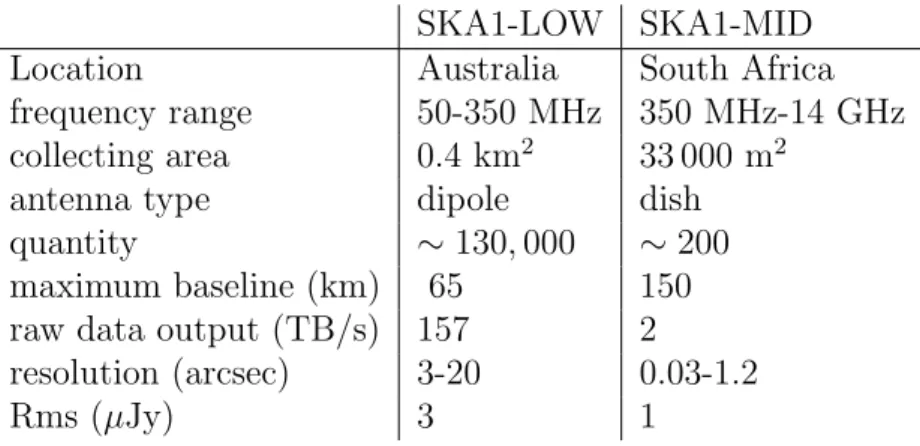
SKA1-LOW SKA1-MID

Location Australia South Africa

frequency range 50-350 MHz 350 MHz-14 GHz

collecting area 0.4 km2 _{33 000 m}2

antenna type dipole dish

quantity ∼ 130, 000 ∼ 200

maximum baseline (km) 65 150

raw data output (TB/s) 157 2

resolution (arcsec) 3-20 0.03-1.2

Rms (µJy) 3 1

Table 2.1: Instrumental parameters of SKA1. The rms is calculated for a 1-hour observation, considering the whole band.

2.2 ASKAP

ASKAP is a radio interferometer, located at Murchison Radio-astronomy Observatory (MRO), in West Australia. In his final shape, it will consist of 36 antennae (see Fig. 2.1), each 12 metres in diameter, positioned in a pseudo-random way to optimise the uv plane coverage (see Fig. 2.2). It covers all the frequencies between 700 and 1800 MHz in 4 bands (3 nowadays, that leave a band-hole between 1300 and 1500 MHz), each 300 MHz wide divided into 16000 channels (there is some overlap). Actually, there are 12 antennae working, in the array called ASKAP-12, that just started the early science. The most innovating devices in ASKAP are the receivers, called Phased Array Feed (PAF), consisting of 188 elements, 94 in each polarisation (see Fig. 2.3). The elements work as an aperture array, whose signal is directly modulated onto optical fibre link that can transverse several kilometres to the digital receiver and the beamformer in the control building (Chippendale et al., 2015). For each antenna, the beamformer combines the digital signal of all the elements of the PAF in order to build 36 beams, each one with a

∼ 1 deg2 _{area at 1.4 GHz, that overlaps and form a ∼ 30 deg}2 _{field of view}

(FOV) (see Fig. 2.41_{). Thanks to this huge FOV, ASKAP will be the fastest}

survey telescope at his wavelength.

1

(33)

Figure 2.1: The ASKAP site from captured from an helicopter.

2.3 EMU

The Evolutionary Map of the Universe (EMU) is a deep blind survey of all

the southern sky up to a declination of +30◦ (75% of the sky). The rms will

be 10 µJy, so, adopting a 5σ detection limit, we will detect all the sources brighter than 50µJy. The expected angular resolution is 10 arcSection The observations will take 2 years and they will be carried out at 20 cm, in the 1120-1420 MHz band.

EMU will provide a whopping 70 millions detections of galaxies, a number ∼ 30 times higher than the total number of galaxies knows nowadays, to a redshift as high as 6 (see Fig. 2.5 for the expected distribution; Norris et al. 2015). Half of the galaxies are expected to be AGN while the others will be normal galaxies (the radio sky is not dominated by AGNs at this sensitivity; Norris et al. 2011). The key science goals for EMU are:

1. trace the evolution of the universe from z = 2 to the present, using the galaxies;

2. trace the evolution of AGNs and supermassive black holes in our uni-verse;

3. use the distribution of the source to do cosmological studies;

4. explore a new region of the phase space, willing to find new classes of objects;

(34)

Figure 2.2: ASKAP antennae configuration and corresponding uv plane in a 12 minute observation.

(35)

(36)

(37)

CHAPTER 2. NEXT GENERATION TELESCOPES AND SURVEYS 36 5. create the larger atlas of the Galactic continuum emission in the

south-ern emisphere.

Even if most of the goals are extra-galactic oriented, EMU will observe a large portion of the Galactic Plane so, based on what NVSS (see the Introduction) did, there will be a huge impact of EMU on it. Goals of the galactic science include:

1. a complete catalogue of all the massive stars in their early stages; 2. a better understanding of the complex structure of giant H ii regions

and how the star formation is triggered in the inside;

3. a more complete catalogue of supernovae remnants, especially the most compact one;

4. detections of planetary nebulae, which can help estimate the rate for-mation of the smaller stars;

5. detections of radio stars and pulsars; 6. discover the unexpected.

We are interested, for this thesis, in the fifth point, the detections of radio stars. EMU, thanks to its sensitivity, is expected to detect a large amount of stars of different classes. EMU will be the first blind survey for stars, allowing us to overcome the problem that all the stars known as radio emitters so far have been detected with targeted observation. In Fig. 2.6 and in Fig. 2.7 it is shown the flux density of the radio star classes described in the Chapter before as a function of, respectively, the frequency and the distance from the observer, after imposing the luminosities of the stellar classes found in Umana et al. (2015a). To estimate the radio stars density that we will find in EMU and how many of them will belong to the different star classes and to approach the issues arising from a so deep survey into the GP, we have started the Stellar Continuum Originating from Radio Physics in Ourgalaxy (SCORPIO; Umana et al. 2015b, hereafter paper I).

(38)

Figure 2.5: Expected redshift distribution of the EMU sources. RQQ are radio quiet quasars, FR1 and FR2 are the Fanaroff-Riley galaxies type 1 and 2.

(39)

Figure 2.6: Average spectrum of common radiostars classes. The WR-OB and giant stars are assumed to be at 1 kpc, the MCP at 0.5 kpc, the RS CVn, flare stars and sun-like stars at 10 pc and the Ultra Cool Dwarf (UCD) at 20 pc. The pale blue horizontal lines represent the SKA-1 1 σ for an hour of observation at the three different bands.

(40)

Figure 2.7: Expected flux of common radio stars classes versus their distance from the Earth at 5 GHz. The pale blue horizontal line represents the SKA1 1σ 1-hour observation.

(41)

Chapter 3 How many radio stars can we

detect?

The next years are going to be crucial for radio astronomy, with several new telescopes that will start working, e. g. the Square Kilometre Array (SKA), the Australian SKA Pathfinder (ASKAP) and MeerKAT. These instruments will be capable of surveying large areas of the sky with high sensitivity, discovering a lot of new radio sources (e.g. the Evolutionary Map of the Universe, EMU, survey will detect 70 millions of galaxies, Norris et al. 2011), and, among them, a lot of radio stars. A method to estimate the number density of radio stars is an application of the Besan¸con model (Robin et al., 2003) to evaluate how many stars per square degree there are in our Galaxy in a given direction. In this chapter we present the results.

3.1 Modelling the Milky Way

This section is based on Mihalas & Binney (1981) and Robin et al. (2003). When we look at the sky with our naked eye we can see a fairly uniform distribution of bright stars over the entire sky and a quite uniform light coming from a plane, the Galactic Plane, caused by billions of fainter stars. We can describe this distribution quantitatively using the star counts. Let A (m, l, b, S) be the number of stars of spectral type S at apparent magnitude m, per unit magnitude interval, per square degree, in galactic coordinates (l, b). We can also determine an integrated star count N (m, l, b, S), the cu-mulative number of stars, per square degree, having apparent magnitudes less than or equal to m. These quantities are observable and are very important for the construction of the Milky Way model. Our ultimate objective is to

determine the space density ν (r, l, b, M, S) (stars pc−3) of stars of absolute

(42)

magnitude M and spectral type S at distance r from the Sun, in the direction selected by galactic coordinates (l, b). For the sake of brevity we shall drop the variables l and b in our notation, every other analysis will be carried out for a definite field with a specific l and b. Assuming that ν (r, M, S) can be

represented as the product of two factors DS(r) and Φ (M, S), we can write:

ν (r, M, S) dM dV = Φ (M, S) dM DS(r) dV (3.1)

where dV is a volume element, dM is an increment of absolute magnitude,

DS(r) is called the relative density function and it represents the density of

stars of spectral type S at distance r and Φ (M, S) is the luminosity function and it gives us the actual number of stars having absolute magnitude M and spectral type S per cubic parsec in the solar neighbourhood. We can also define the general luminosity function

Φ (M ) ≡

S

Φ (M, S) (3.2)

This function describes the stellar composition of a unit volume in the solar neighbourhood at the present time. However the distribution of stars over luminosity implied by Φ (M ) is not an accurate representation of the relative frequencies with which these stars are formed. This is caused by the rapid

decrease of the main-sequence lifetime τM S(M) of stars with increasing mass

M. Therefore, below some critical mass M0, stars will persist on the main

sequence for periods longer than τG, the age of our Galaxy, while stars with a

mass exceeding M0 will evolve as white dwarf or explode as supernova. This

effect leads to a great abundance of low-mass, faint stars. To describe the rate of star creation it was introduced by Salpeter (1955) an initial luminosity

function Ψ(MV) which gives the relative numbers of stars formed, per unit

magnitude interval per unit volume as a function of MV.

In the broadest term, our Galaxy comprises two main structural elements, a spheroidal component and a disc (see Fig. 3.1 for a complete scheme). The first one can be thought of as being an approximately axially symmetric system that can be divided into several subcomponents: the nucleus, the innermost part of the Galaxy, with a size of ∼ 3 pc, the bulge, ∼ 3kpc in size, and the extensive halo around our Galaxy, that can extend to a radius of ∼ 30 kpc or more. The disc can be divided into two subcomponents: the thin disc, that is an extremely thin (about 200 pc thick), flat system extending in the Galactic Plane from the center to a radius of 25 ∼ 30 kpc and the thick disc that is about 2 kpc thick but it is less dense.

The spheroidal component is almost gas and dust free. The stars that are part of it are usually metal-poor subdwarfs and RR Lyrae variables. Both the

(43)

CHAPTER 3. HOW MANY RADIO STARS CAN WE DETECT? 42 star density and the metallicity rise considerably toward the Galactic centre, leading scientists to divide the spheroidal stellar population into a sequence of subpopulations, such as bulge-component stars, intermediate spheroidal-component stars and halo-spheroidal-component stars. They have low orbital velocity around the galactic centre and high eccentricity. The disc is usually divided into two subcomponents, the thin disc and the thick disc. The thin disc component is constituted by: interstellar dust and gas, young metal-rich stars, which are concentrated on the spiral arms and older metal-rich stars which have a smooth distribution throughout the disc. Thin disc stars have high rotation velocity and almost perfectly circular orbit. The thick disc is composed of older stars and there are several theories about its genesis:

1. it comes from the heating of the thin disc (Steinmetz, 2012);

2. more energetic stars migrate outwards from the inner galaxy to form a

thick disk at larger radii (Sch¨onrich & Binney, 2009);

3. it is a result of a merger event between the Milky Way and another dwarf galaxy (Bensby & Feltzing, 2010);

4. the disc forms thick at in the first ages of the universe with the thin disc forming later (Brook et al., 2004).

The thick disc stars are poorer in metals than the thin disc ones and they are studied for determining the chemical composition of the Galaxy in early time.

Models divide stars into several populations, corresponding to their posi-tion in the different elements of the Galaxy, each one described with several

parameters such as age, metallicity F e_H, initial mass function (IMF), star

formation rate (SFR), density law, local mass density, etc.

3.2 The Besan¸

con model

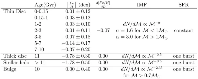
In this section we discuss the Besan¸con model (Robin et al., 2003). They divide stars into 4 populations: disc, thick disc, stellar halo and bulge. To compute the population synthesis model, the stellar content at each epoch has been extracted from standard parameters such as the IMF, SFR and a set of evolutionary track (see Table 3.1).

The thin disc population was assumed to evolve in 10 Gyr, life-span de-rived from the white dwarf luminosity function with an accuracy of about 15% (Wood & Oswalt, 1998). Sets of IMF slopes and SFRs have been ten-tatively assumed and tested against star counts. The luminosity function

(44)

Figure 3.1: Components of our Galaxy Age(Gyr) F e H  (dex) d[F e/H] dR IMF SFR Thin Disc 0-0.15 0.01 ± 0.12 0.15-1 0.03 ± 0.12 1-2 0.03 ± 0.10 dN/dM ∝ M−α 2-3 0.01 ± 0.11 −0.07 α = 1.6 for M < 1M⊙ constant 3-5 −0.07 ± 0.18 α = 3.0 for M > 1M⊙ 5-7 −0.14 ± 0.17 7-10 −0.37 ± 0.20

Thick disc 11 −0.78 ± 0.30 0.00 dN/dM ∝ M−0.5 one burst

Stellar halo > 11 −1.78 ± 0.50 0.00 dN/dM ∝ M−0.5 one burst

Bulge 10 0.00 ± 0.40 0.00 dN/dM ∝ M−2.35 one burst

for M > 0.7M⊙

Table 3.1: Age, metallicity, radial metallicity gradient, initial mass function and star formation rate of the stellar components.

(45)

CHAPTER 3. HOW MANY RADIO STARS CAN WE DETECT? 44 derived by the data of the Hipparcos mission (Perryman et al., 1997) con-strained the following parameters:

1. The IMF is modeled by a broken power law (see Table 3.1). At high

masses the slope of the function dN/dM ∝ M−α is assumed to be

α = 3, steeper than the Salpeter assumption, and it is determined by Haywood, Robin, & Creze (1997), while at low mass the assump-tion α = 1.6 was chosen to better fit the Jahreiß luminosity funcassump-tion (Jahreiss, 2003);

2. new constraints on the local kinematics made them choice the age-velocity dispersion relation from Gomez et al. (1997);

3. the local density of interstellar matter is set to 0.021M⊙pc−3 from the

Dame (1993) observation of the local surface density of Hi+H2, which

leads to a total local mass density of 0.076 ± 0.015M⊙pc−3 as in Cr´ez´e

et al. (1998).

As already stated, there are several thick disc formation scenario theories. A formation by a merger event was assumed for this model, which explains the observed properties of this population: the accreting body heats up the stellar population previously formed in the disc making a thicker population with larger velocity dispersion. The thick disc abundances are intermediate between the stellar halo and the thin disc. They also assumed a single epoch of star formation, that cannot exceed 1 Gyr and that took place 11 Gyr ago. The stellar halo and the Bulge are distinct in the model construction but they may be related in their formation scenario. The most significant difference in the model between the two populations is the abundance dis-tribution. In fact, while halo stars are assumed to be metal-poor, the bulge stars, despite being ∼ 10 Gyr old, have a higher metal concentration. To have a more detailed description of the model see Robin et al. (2003).

3.3 Radio stars counts

In order to estimate the number of radio stars that can be detected with the new surveys, we used the Besan¸con model, which gives us the number of stars of a given spectral type, at distance r from the Sun, for the direction (l, b). While its purpose is to simulate an optical stellar field, we want to simulate a radio one. To achieve this goal, given that the Galaxy is optically thin at radio wavelengths, we set the diffuse emission parameter to A = 0 and, to collect all the stars in a given direction, we imposed 30 as the faintest magnitude to detect. Among all the stars that can emit in radio we decided

(46)

to investigate only the most common ones: the M stars, the OB stars and the MCP stars. We will also discuss the RS CVn binary stars but we will not use the Besanc¸con model for that. To show our results, we assume a quantity N (S) that is defined as the number of source per square degree having a flux that exceeds S and we plot the log N -log S distribution figure.

3.3.1 OB and Wolf-Rayet stars

The star formation, as explained before, is a process localised in the thin disc. Stars can move from the thin disc but it is a really long process. OB and Wolf-Rayet stars are intrinsically bright and quite young among the stars, so we supposed the distribution to be anisotropic, with almost all the stars lying in the GP (Mihalas & Binney, 1981). We set the maximum distance along the GP to be 20 kpc. We proceeded to simulate the number of stars of each spectral type and luminosity class from O4 to B3 (see Table 3.2 for the used parameters), dividing the GP longitudinally in 60 degrees interval and latitudinally in −1 < b < 1, 1 < b < 3, 3 < b < 23, assuming that we should have a similar star density at opposite latitude. We assumed the OB stars to emit radio waves because of the free-free mechanism in their wind. OB stars have high values of mass loss caused by their radiation pressure Garmany & Conti (1984):

log ˙M = −6.2 + 1.6 (L/L⊙− 5) − 0.5 log (M/M⊙(1 − Γ)) (3.3)

where L is the optical luminosity of the star, M the mass and Γ = σeL

4πGM c is

the ratio of stellar luminosity to the Eddington limit, σeis the cross section of

the electron, G and c are respectively the gravitational constant and the speed

of light. ˙M is expressed in M⊙yr−1. The mass loss generates an ionized wind

around the star which has a density proportional to r−2 (assuming the wind

velocity constant and a spherical symmetry) and that emits as in Panagia & Felli (1975): S = 5.12 ν 10 GHz 0.6 T_e 104_K 0.1 ˙ M 10−5_M ⊙/y 4₃  µ 1.2 −4₃  v_exp 103_{km s}−1 −4₃ ¯ Z23d−2 kpc (3.4)

where ν is the frequency, M is the mass of the star, dkpc is the distance in

kpc, µ and ¯Z are the average atomic number and the average charge of the

(47)

CHAPTER 3. HOW MANY RADIO STARS CAN WE DETECT? 46

Figure 3.2: log N -log S distribution for a galactic latitude −1 < b < 1 at different galactic longitude. The black line is at 50 µJy, the EMU sensitivity, while the blue one is at 1 µJy, the SKA-1 25-hours sensitivity.

Figure 3.3: Density of OB stars with a flux greater than 1 µJy for −1 < b < 1, 1 < b < 3 and 3 < b < 23 with respect to galactic longitude.

(48)

3. HO W MANY R A DIO ST ARS CAN WE DETECT? 47 SP Teff (K) Mv L/L⊙ Mass/M⊙

ZAMS-V III I ZAMS V III I ZAMS V III I

O4 50000 47500 45000 −6.1 −6.1 −6.3 −6.5 6.11 6.11 6.12 6.13 35 O5 47000 44500 42000 −5.6 −5.8 −6.0 −6.4 5.83 5.92 5.93 6.00 32.7 O5.5 44500 42500 40000 −5.2 −5.5 −5.8 −6.3 5.60 5.74 5.78 5.89 31 O6 42000 40000 38000 −4.9 −5.3 −5.6 −6.3 5.40 5.56 5.63 5.82 29.5 O6.5 40000 38000 36000 −4.5 −5.0 −5.5 −6.3 5.17 5.37 5.50 5.75 29 O7 38500 36500 35000 −4.2 −4.8 −5.5 −6.3 5.00 5.24 5.45 5.72 28.3 O7.5 37500 35500 34000 −4.1 −4.6 −5.5 −6.4 4.92 5.11 5.41 5.73 26 O8 36500 34500 33000 −3.9 −4.5 −5.5 −6.5 4.81 5.05 5.38 5.74 25.2 O8.5 35500 33500 32000 −3.8 −4.4 −5.5 −6.6 4.73 4.97 5.35 5.75 23 O9 34500 33000 31000 −3.7 −4.3 −5.5 −6.7 4.66 4.90 5.34 5.76 22.6 O9.5 33000 31500 30000 −3.6 −4.2 −5.5 −6.7 4.58 4.82 5.30 5.73 20 B0 30900 29300 28000 −3.3 −4.0 −5.0 −6.6 4.40 4.68 5.03 5.63 17.8 B0.5 26200 25000 23600 −2.8 −3.5 −4.3 −6.6 4.04 4.31 4.57 5.48 14 B1 22600 21500 20400 −2.3 −2.9 −3.8 −6.6 3.72 3.95 4.27 5.32 11.7 B2 20500 19500 18500 −1.9 −2.5 −3.6 −6.8 3.46 3.70 4.09 5.28 10.0 B3 17900 17000 16100 −1.1 −1.7 −3.1 −6.8 3.02 3.24 3.75 5.20 7.32

Table 3.2: Typical OB stars parameters from Panagia (1973). ZAMS is the zero main sequence, V, III and I are the luminosity class of dwarf, giant and hypergiant.

(49)

CHAPTER 3. HOW MANY RADIO STARS CAN WE DETECT? 48 In Fig. 3.2 the log N -log S distribution of OB stars along the Galactic Plane (−1 < b < 1) is shown, while in Fig. 3.3 the number of stars with a flux greater than 1µJy (the sensitivity of 25-hours SKA-1) versus l at different b at 5 GHz is shown. As expected, the number of OB stars decreases rapidly going away from the Galactic Centre. Notice that we are taking into account the wind radio emission of the OB stars, however a lot of them (∼ 20% of the O stars) are embedded in nebulae, so what we will see are Hii regions and not stellar winds. Is it possible for the stellar wind to completely absorb the UV radiation of a OB star and to block the formation of an Hii region, or at least diminish its area? We will consider a typical O4V star and compute

how many photons its wind will block. We know that ˙M = 4πr2_{ρv, where ρ}

is the density of the wind and v its velocity, so we have:

ρ = M˙

4πr2_v

Assuming v = 1000 km s−1 and ˙M = 10−5M⊙we will have ρ ≈ 6·109protons

cm−3 at r = 10R∗, where R∗ = 10R⊙. The number of absorbed photons is

Nr = βrρ2, so Nr ≈ 107 photons cm−3 s−1 and the entire surface will absorb

nr = Nr· 4πr2 = 6.8 · 1033 photons cm−1 s−1. In total we will have

nr(r) = 6.8 · 1033  10R∗ r 2 ⇒ Ntot =  ∞ 2R∗ N (r) dr

so Ntot = 2.4 · 1047 photons s−1, negligible with respect of the ∼ 1050 photons

s−1 emitted by the star.

3.3.2 MCP stars

MCP (or CP2) stars, as OB and Wolf-Rayet, are intrinsically bright and quite young, so we supposed the distribution to be anisotropic, with almost all the stars lying in the GP (Mihalas & Binney, 1981). Only 25% of all the MCP emits in radio wavelength (Leone, Trigilio, & Umana, 1994) so, after simulating the number of main sequence stars of each spectral type between B8 and A7, the fraction of them supposed to be MCP are reported in Table 3.3 and their 25% are assumed to be radio emitters. Assuming a

typical MCP radio luminosity of 1016.8±0.9 _{erg s}−1 _Hz−1 _{(Drake et al. 1987;}

Linsky, Drake, & Bastian 1992) at 5 GHz, we derived the expected log N -log S distribution for CP stars in Fig. 3.4 and the spatial distribution at a 1µJy/beam sensitivity in Fig. 3.5.

(50)

Figure 3.4: log N -log S distribution for a galactic latitude −1 < b < 1 at different galactic longitude. The black line is at 50 µJy, the EMU sensitivity, while the blue one is at 1 µJy, the 25-hours SKA-1 sensitivity.

Spectral Type Ntot MCP Percentage of the total

B8-B9 1916 327 17%

A0-A1 2014 191 9%

A2-A3 1728 58 3%

A4-A5 650 6 1%

A6-A7 303 16 5%

Table 3.3: Number of total stars Ntot and number of MCP at every spectral

A Pathway to EMU: the SCORPIO Project

Universit`

a degli studi di Catania

A Pathway to EMU:

The SCORPIO Project

PhD Thesis

Contents

List of Tables

List of Figures

Chapter 1

Introduction

1.1

Radio sources

1.1.1

Emission mechanism

1.1.2

Extra-galactic sources

1.1.3

Galactic sources

18h46m44.40s

46.20s

RA (J2000)

45.0"

30.0"

15.0"

45'00.0"

45.0"

-0°44'30.0"

Dec (J2000)

1.2

Work outline

Chapter 2

Next generation telescopes and

surveys

2.1

SKA

2.2

ASKAP

2.3

EMU

Chapter 3

How many radio stars can we

detect?

3.1

Modelling the Milky Way

3.2

The Besan¸

con model

3.3

Radio stars counts

3.3.1

OB and Wolf-Rayet stars

3.3.2

MCP stars