SAMPLING PROPERTIES OF THE DIRECTIONAL MOBILITY
INDEX AND THE INCOME OF ITALIAN FAMILIES
Camilla Ferretti1
Dept. of Economics and Social Sciences, Univ. Cattolica del Sacro Cuore, Piacenza, Italy
1. Introduction
In literature, transition matrices have been widely used to describe the dynamics of discrete state processes based on economic variables. In this sense relevant examples are, among others, the analysis of flows of individuals in the labor market (Fougere and Kamionka, 2003), of firms among size classes (Cipollini et al., 2012), or of citizens among income levels (Bourguignon and Morrison, 2002). Any given transition matrix P ={pij}i,j=1,...,kprovides all the information on the movements
of individuals among the states (labeled with 1, . . . , k), since pij usually is the
conditional probability of moving in j at time t, given the state i at time t− 1. Assuming appropriate hypothesis (for example, P is ruling transitions in a Markov Chain), the knowledge of P permits to forecast the evolution of individuals among the k states.
We shortly introduce the theory of mobility indices considering the set of the transition matrices with k states, with k∈ N+:
P = P = (pij)∈ Rk×k|pij ≥ 0, k ∑ j=1 pij = 1,∀ i = 1, . . . , k .
A given matrix P can be associated to a certain degree of mobility through a synthetic mobility index I(P ). The larger is I(P ), the higher is the degree of mobility in the group of individuals ruled by P . Mobility indices for transition matrices are then functions I(·) mapping a given transition matrix P ∈ P in the value I(P )∈ R. As specified in Ferretti (2012), mobility indices introduce a total order ”≺” in P, that is a rule which permits to establish unequivocally if the mobility of P is lower/higher than the mobility of Q, for every couple P, Q∈ P. Basically, chosen the function I(·), we say that P ≺ Q (”P is less mobile than Q”) if and only if I(P ) < I(Q). It is worth noting that the order inP depends on the choice of I(·).
Famous proposals for the function I(·) are, among others, in Shorrocks (1978), Sommers and Conlinsk (1979), Bartholomew (1982) and Geweke et al. (1986). As an important example of I(·) we are going to use in the following, we recall here the trace index (Prais, 1955; Shorrocks, 1978):
Itr(P ) = k−∑ki=1pii k− 1 = ∑k i=1(1− pii) k− 1 .
The trace index furnishes an absolute measure of the mobility: in particular it measures the global tendency to leave from the current state, since 1− pii is the
probability to move away from the i-th state.
In Ferretti and Ganugi (2013) we proposed a new mobility measure, the directional index : Idir(P ) = ∑ i ωi ∑ j pij· sign(j − i) · v(|j − i|). (1)
Idir derives from the necessity to compare different evolutions when the set of
states is ordered from the worst (state ”1”) to the best one (state ”k”) as in the case of incomes or firm size. Idir(P ) is then a real value which is positive when
the prevailing direction of individuals is towards the better states, and negative in the opposite case.
The directional index is also provided with some parameters: 1) ωi, i = 1, . . . , k
are weights to be assigned to individuals starting from the i-th state (we assume ωi ≥ 0 for every i and
∑k
i=1ωi = 1); 2) v is a not-decreasing function such that
v(0) = 0 and v > 0 otherwise. It measures the contribute to the whole mobility of individuals making jumps of magnitude|j − i|. In the end, the function sign is defined as follows: sign(x) = +1, if x > 0; −1, if x < 0; 0, if x = 0;
and gives a positive (resp. negative) sign to jumps which lead to a better (resp. worse) state than the current one. For sake of shortness, we will indicate herein sign(j− i) · v(|j − i|) with vij.
In the past works we found that for any P ∈ P, given {ωi} and v, Idirassumes
values in [m1, m2], where m1= ∑k
i=1ωivi1≤ 0 and m2= ∑k
i=1ωivik≥ 0 (Ferretti
and Ganugi, 2013, p. 414). In the light of that, we also proposed to use the normalized version I∗ of Idir:
I∗(P ) = {
Idir(P )/m2 if Idir(P )≥ 0;
−Idir(P )/m1if Idir(P ) < 0;
(2)
which belongs to [−1, +1] for every choice of ω and v. Note that normalization is always possible. In fact we have m1= 0 if and only if ω = (1, 0, . . . , 0). In this case we have Idir ≥ 0 for every P ∈ P and it is normalized dividing by m2= v1k > 0. If m2= 0 analogous results hold. From a descriptive point of view, I∗ simplifies the comparison of two matrices, since its extreme values are univocally defined, and intermediate values of mobility can be considered as a percentage.
Aim of this paper is to carry on the analysis of the directional index, facing the problem of its statistical properties. In the following we will assume the existence of an underlying theoretical model, observed through a sample of size n. In particular we suppose that the movements among the states are ruled by a Markov Chain with unobservable transition matrix P . Following the ideas proposed in Schluter (1998) and Formby et al. (2004), we derive the asymptotic sampling distribution of Idir( ˆP ), where ˆP is the estimate of P .
The paper is organized as follows: Sect. 2 recalls some important results about the asymptotic sampling distribution of ˆP and proves that Idir( ˆP ) is
asymptot-ically normally distributed; Sect. 2.3 reports the results of a numerical example which support the asymptotic Normality of the sampling directional index; Sect. 3 shows the analysis of mobility of four samples of Italian families provided by Banca d’Italia for the years 2004-2012. The last section contains comments and possible further developments.
2. Asymptotic sampling distribution
We then consider the case of an unobservable P ∈ P which rules a Markov chain among k states. Mobility is measured on samples of size n and the function I(·) is evaluated on the estimated ˆP . In literature there exist some results about the sampling distribution of the ˆpij. In particular we will refer to the seminal paper
of Anderson and Goodman (1957). Statistical procedures will be applied on ˆIdir
instead of ˆI∗ because, being the latter a piecewise linear function of the former, we may run into some problems in the variance calculus, especially if I∗(P ) = 0. Nevertheless tests results on ˆIdir can be extended to ˆI∗ exploiting the fact that
I∗(P ) = 0 if and only if Idir(P ) = 0. The normalized directional index will be
shown to make easier the descriptive comparison between different samples.
2.1. One observed matrix
We suppose to have at disposal observations about two consecutive instants of time t0 and t1. On such basis we build the k× k empirical matrix X such that xij is the number of individuals being in state i at time t0 and in state j at time
t1. It holds
k
∑
j=1
xij = ni= nr. of individuals starting from i
and k ∑ i,j=1 xij = k ∑ i=1
ni = n = size of the sample.
In this case the MLE estimator ˆP of P has elements ˆ
pij =
xij
ni
, (3)
Let xi= (xi1, . . . , xik) be the observed vector of individuals moving from i. It
is proved that
xi∼ Multinomial(pi, ni),
where pi = (pi1, . . . , pik). Consequently ˆpi = (ˆpi1, . . . , ˆpik) is asymptotically
dis-tributed as a multivariate Normal N (pi, Σ), where Σ has elements:
Σjl= cov(ˆpij, ˆpil) = { pij(1−pij) ni if j = l; −pijpil ni if j̸= l.
(Rows of P are still supposed to be independent one from the each others, and ni
is supposed to be known for every i = 1, . . . , k).
The sampling directional index is then asymptotically distributed as a Normal with mean µ(Idir( ˆP )) and variance σ2(Idir( ˆP )). We have that
µ(Idir( ˆP )) = Idir(P ). (4)
This condition of unbiased estimator is valid also for finite n, since it is a direct consequence of the linearity of the expected value.
The formula of σ2(I
dir( ˆP )) needs some additional computation. We firstly
compute the variance of ˆIi= Ii( ˆP ), where
Ii(P ) = ∑ j pij· vij. σ2( ˆIi) = σ2 ∑k j=1 ˆ pijvij =∑k j=1 σ2(ˆp ijvij) + 2 k ∑ l=j+1 Cov(ˆpijvij, ˆpilvil) = = k ∑ j=1 pij(1− pij) ni · v 2 ij− 2 k ∑ l=j+1 pijpil ni · v ij· vil .
From the independence between Ii and Ij, the final variance of I( ˆP ) is given by
σ2(Idir( ˆP )) = σ2( ∑ i ωiIi( ˆP )) = ∑ i ωi2σ2( ˆIi). (5)
2.2. Two or more observed matrices
In many cases, relevant economic variables are observed in more than two consecu-tive instants of time: t0, . . . , tT. Usually we consider equi-spaced instants of time,
indicating them simply with 0, 1, ..., T . Coherently with the previous section, let xij(t) be the number of individuals being in the i-th state at time t− 1 and in the
j-th state at time t, for every t = 1, . . . , T . Entries of P are in this case estimated with: ˆ pij= ∑T t=1xij(t) ∑T t=1 ∑k j=1xij(t) . (6)
Note that the time-homogeneity of Markov Chains is here needed, that is the model of the transitions is the same in every step from t− 1 to t, t = 1, . . . , T .
As before, we consider the number of individuals being in the i-th state at time t, for t = 0, . . . , T : ni(t) = k ∑ j=1 xij(t),
and the number of individuals passing from i before time T :
n∗i =
T∑−1 t=0
ni(t).
Following again Anderson and Goodman (1957), we prove that ˆ
pi asym.
∼ N (pi, Σ∗),
where Σ∗ has elements:
Σ∗jl= cov(ˆpij, ˆpil) = { p ij(1−pij) n∗i if j = l; −pijpil n∗i if j̸= l.
Consequently, Idir( ˆP ) is asymptotically distributed as a Normal with expected
values equal to Idir(P ) and variance obtained by Eq. (5) simply substituting ni
with n∗i.
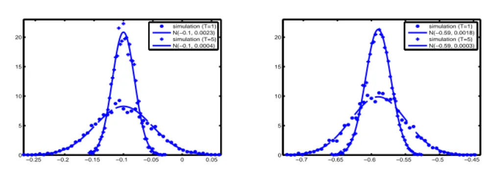
2.3. Simulation
The purpose of the following numerical example is to support the Normality of the asymptotic distribution. We consider the randomly chosen theoretical matrix
P = .2 .3 .1 .4 .3 .5 .1 .1 .2 .4 .4 0 .1 .2 .6 .1 .
Our data consist in 5000 simulated realizations of the corresponding homogeneous Markov chain. For any simulation we set n = 500 (the number of individuals), with the given starting frequencies p0= (.2, .1, .3, .4). In the first case we consider T = 1, in the second case T = 5. Consequently ˆP is estimated as in Eqs. (3) and (6).
We evaluate Idir( ˆP ) setting v(|j −i|) = |j −i|, which gives a linearly increasing
weight to jumps from i to j, as specified in the following section. We also analyze two different cases for the weights ωi: on one hand we suppose that the starting
state gives no information about the mobility, that is ω = (.25, .25, .25, .25); on the other hand we choose ω = (.1, .2, .3, .4), which means that individuals in the 4-th
−0.25 −0.2 −0.15 −0.1 −0.05 0 0.05 0 5 10 15 20 simulation (T=1) N(−0.1, 0.0023) simulation (T=5) N(−0.1, 0.0004) −0.7 −0.65 −0.6 −0.55 −0.5 −0.45 0 5 10 15 20 simulation (T=1) N(−0.59, 0.0018) simulation (T=5) N(−0.59, 0.0003)
Figure 1 – Simulated versus theoretical density distribution of I∗( ˆP ), with ω =
(.25, .25, .25, .25) (left) and ω = (.1, .2, .3, .4) (right).
state carry more weight than others in the global mobility measure2. We obtain Idir(P ) =−0.1,
when ω = (.25, .25, .25, .25), and
Idir(P ) =−0.59,
when ω = (.1, .2, .3, .4). In both the cases we find that the mobility is negative, that is individuals mainly tend to move towards left (i.e. to make their condi-tion worse, as for example families evolving among income classes and moving towards the smaller classes). If we would compare the two measures without sta-tistical procedures, a better choice is the evaluation of their normalized versions. Respectively we find I∗=−0.067 (-6.7%) and I∗=−0.295 (-29.5%).
Figure 1 shows the results of our simulation for T = 1 and T = 5. We compare the simulated density distribution of the index (built up using 50 class intervals) and the Normal density distribution with expected value and variance calculated as in Eqs. (4) and (5). The graphical comparison supports the Normality of the sampling index. Table 1 instead contains the theoretical and simulated values for the mean and the variance of Idir( ˆP ). We display also the p-value obtained with
the Shapiro-Wilk test of normality, which still confirms our results.
3. An empirical illustration
As an empirical illustration of the previous results, we propose the analysis of the mobility of Italian families subdivided according with their income. We aim to rigorously determine if mobility among income classes before and after the crisis is negative, positive, or equal to zero, and if it has significantly changed in
2
As explained in Ferretti and Ganugi (2013), we may need to make distinction among different states. For example, in the empirical application it is useful to give more weight to states with more individuals, by setting ω equal to the starting frequency distribution
TABLE 1
Comparison between simulated and theoretical mean and variance, and Shapiro-Wilk test’s p-value for Normality.
µ( ˆIdir) simulated mean σ2( ˆIdir) simulated variance p-value ω = (.25, .25, .25, .25) T = 1 -0.1 -0.0998 0.0024 0.0023 0.1787 T = 5 -0.1 -0.0997 0.0004 0.0004 0.5074 ω = (.1, .2, .3, .4) T = 1 -0.59 -0.5909 0.0018 0.0016 0.6756 T = 5 -0.59 -0.5901 0.0004 0.0003 0.5027 TABLE 2
Income classes for Italian families (Euros).
q1 q2 q3 q4 q5
[0; 17097) [17097; 24453) [24453; 34036) [34036; 48762) [48762; +∞)
the time. For our proposals we use the data provided every two years by Banca d’Italia, focusing on the surveys about the two-years periods 2004-2006, 2006-2008, 2008-2010 ad 2010-2012 (Banca d’Italia, 2008, 2010, 2012, 2014) and we build the sampling transition matrices using five classes q1, . . . , q5 delimited by the 2004-quintiles and displayed in Table 2. To avoid the bias caused by the inflation we convert the observed incomes into the 2013 values using the ISTAT revalorization’s coefficients (http://www.istat.it/it/archivio/30440).
The estimated matrices are obtained as in Eq. (3), and they are shown in Table 33.
As a first descriptive step we evaluate the trace index (Table 4). We see that the ”turbulence” tends to decrease until 2010, that is Italian families undergo a decline of their capacity to move from one class to the others. In 2010-2012 we observe instead an increase in the mobility. At the same time we note the lack of information about the prevailing direction of families.
In the second step we make statistical inference about the directional mobility of Italian families. To evaluate Idir( ˆP ) we set ω equal to the starting distribution of
every two-years span of time (last column of Table 3). The parameter v is instead needed to give more weight to larger jumps. For example, if v ≡ 1, individuals moving from the first to the second class play the same part in the mobility than individuals moving from the first to the third class. If we had geometrically increasing classes, an exponential function of |j − i| would be a suitable choice. Since income intervals do not have a recognizable trend in their size, we choose the simplest way to assign more weight to larger jumps by setting v(|j − i|) = |j − i|.
3The 2004 distribution is not equal to (0.2, 0.2, 0.2, 0.2, 0.2) because quintiles in Table
2 are evaluated on the whole 2004’s sample (8012 families) , and matrices are estimated on the 3957 families which appear in both the 2004’s and the 2006’s samples.
TABLE 3
Estimated income transition matrices for the years 2004-2006, 2006-2008, 2008-2010, 2010-2012 (values are expressed as percentages).
Income in the final year
Income in the initial year q1 q2 q3 q4 q5 p0
2004-2006 (n = 3957) q1 64.10 24.35 7.57 3.44 0.55 18.37 q2 17.10 43.21 27.42 9.27 3.00 19.36 q3 6.35 17.79 41.68 26.18 8.01 19.89 q4 2.42 6.40 18.48 49.15 23.55 20.92 q5 0.71 2.47 6.01 20.26 70.55 21.46 2006-2008 (n = 4345) q1 69.39 22.46 5.21 2.14 0.80 17.22 q2 18.87 52.33 20.38 6.79 1.64 18.30 q3 7.05 21.27 48.90 18.38 4.39 19.91 q4 1.46 5.61 20.27 55.51 17.15 22.14 q5 0.31 1.44 5.74 19.69 72.82 22.44 2008-2010 (n = 4621) q1 73.52 19.09 4.56 1.60 1.23 17.57 q2 19.27 53.82 20.64 5.59 0.68 18.98 q3 5.71 19.21 54.00 17.76 3.32 20.84 q4 1.78 4.95 18.69 56.28 18.30 21.88 q5 0.63 1.36 4.38 19.42 74.22 20.73 2010-2012 (n = 4611) q1 78.75 16.09 3.24 1.68 0.24 18.07 q2 27.21 53.10 15.99 3.10 0.60 18.17 q3 10.44 26.52 45.26 15.34 2.45 20.36 q4 3.05 8.66 25.05 47.86 15.38 21.30 q5 0.88 2.75 6.67 23.75 65.95 22.10
Source: processing of microdata from Banca d’Italia, Indagine sui bilanci delle famiglie italiane.
TABLE 4 Sampling trace indices.
Years 2004-2006 2006-2008 2008-2010 2010-2012
ˆ
Itr 0.5783 0.5026 0.4704 0.5227
TABLE 5
Sampling directional indices and p-values for the one-sample test (H0: Idir(P ) = 0).
Years 2004-2006 2006-2008 2008-2010 2010-2012 ˆ Idir 0.0695 -0.0304 -0.0249 -0.1945 ˆ se 0.0144 0.0124 0.0117 0.0123 p-value 1.30E-06 0.0143 0.0329 0.0000 ˆ I∗ 3.61% -1.42% -1.19% -9.2%
TABLE 6
ˆ
Idir values evaluated on families moving from different income classes.
Starting class 2004-2006 2006-2008 2008-2010 2010-2012 q1 0.5199 0.4251 0.3793 0.2857 ˆ se 0.0304 0.0277 0.0265 0.0219 q2 0.3786 0.2000 0.1460 -0.0322 ˆ se 0.0351 0.0311 0.0275 0.0270 q3 0.1169 -0.0821 -0.0623 -0.2716 ˆ se 0.0357 0.0313 0.0275 0.0303 q4 -0.1498 -0.1871 -0.1563 -0.3615 ˆ se 0.0324 0.0269 0.0264 0.0302 q5 -0.4252 -0.3672 -0.3476 -0.4887 ˆ se 0.0265 0.0220 0.0222 0.0253 TABLE 7
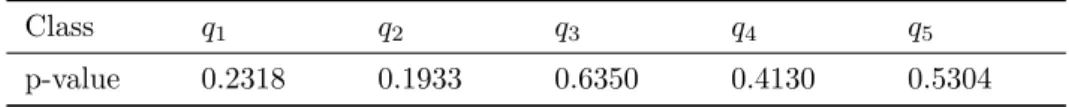
Difference-of-means test’s p-values on 2006-2008 versus 2008-2010.
Class q1 q2 q3 q4 q5
p-value 0.2318 0.1933 0.6350 0.4130 0.5304
Table 5 shows the values of Idir( ˆP ), the estimated standard error and the
normalized values I∗( ˆP ). Mobility is positive in 2004-2006 and assumes negative values in the years over the crisis. Still more relevant is the negative sign joined with an increased absolute value of the index in the last period 2010-2012 (-9.2%). Italian families have then apparently experienced a slowing down in their mobility over the crisis (confirmed by the trace index, too), followed by a stronger worsening of the mean conditions in the last two years. We also apply a difference-of-mean test based on two samples to test ”H0: the mobility has not significantly changed in the time”. H0 is always rejected, except for the couple 2006-2008 and 2008-2010. In this case the corresponding p-value is equal to 0.747. We conclude that from 2006 to 2010 families have undergone a sort of stagnation in their mobility.
In the last step we analyze the mobility restricted to families starting from the i-th class, obtained by setting ω = ei(the i-th canonical vector inRk), i = 1, . . . , 5.
Table 6 contains the sampling directional index ˆIdir restricted to every class,
and the corresponding standard error. From such results we derive the following issues:
1. Mobility is generally significantly different from zero (p-values are not dis-played for shortness). The restricted directional indices confirm the stagna-tion from 2006 to 2010 (Table 7).
posi-TABLE 8
Normalized directional index for income classes.
2004-2006 2006-2008 2008-2010 2010-2012 q1 13% 10.63% 9.48% 7.14% q2 12.62% 6.67% 4.87% -3.22% q3 5.84% -4.10% -3.12% -13.58% q4 -4.99% -6.24% -5.21% -12.05% q5 -10.63% -9.18% -8.69% -12.22%
tive/negative mobility. It is worth noting that the index values are mono-tonically decreasing in time.
3. Families in q2 exhibit a positive mobility except for the 2010-2012 period, whose index is statistically equal to zero (p-value equal to 0.116). Then families in the second class show a tendency to improve their income level. The same tendency is slowing down in the time as for families in q1. 4. Families in q3 and q4 have the worst results. Mobility is always negative
except for the third class in the first period. We note the negative minimum reached in both the classes in the last two years, indicating that families are still suffering the economic crisis. We also note that mobility values show a slight trend reversal in 2008-2010 with respect to 2006-2008, maybe caused by the partial economic recovery happened in 2010.
Lastly, we show the normalized index for families starting from every income class (Table 8). Normalized values of mobility still confirm the previous results. It is interesting to note that, in 2010-2012, families starting from q3, q4 and q5reach similar levels of mobility (around -13%).
4. Conclusions and further research
In this paper we develop an analysis of the sampling distribution for directional mobility index proposed in Ferretti and Ganugi (2013). The index results to be asymptotically Normally distributed, with explicit expression for the expected value and the variance.
The asymptotic distribution of the index allows us to rigorously analyze move-ments of Italian families among income classes, exploiting the sampling microdata provided by Banca d’Italia in the years 2004-2006, 2006-2008, 2008-2010 and 2010-2012. Families are subdivided according with the 2004 income quintiles.
Results show a prevailing tendency to move towards the lowest income classes. Only families starting from the second class (having income comprised between 17097 and 24453 Euros) show a positive behavior, also if their mobility is decreas-ing in the time. A relevant result regards the 2010-2012 mobility: in this span of time families in the last three classes (that is having income greater that 24435 Euros) show a negative minimum in their mobility value (around -13%).
Further researches will regard the update of the analysis using more recent data. From a theoretical point of view we aim to extend the theory of direc-tional indices, and the related statistical inference, to more refined models, such as mixtures of Markov Chains and continuous-in-time models.
References
T. W. Anderson, L. A. Goodman (1957). Statistical inference about markov chains. The Annals of Mathematical Statistics, 28, no. 1, pp. 89–110.
Banca d’Italia (2008). I bilanci delle famiglie italiane nel 2006. Supplementi al bollettino statistico. URL https://www.bancaditalia.it/pubblicazioni-/indagine-famiglie/bil-fam2012/suppl 07 08.pdf.
Banca d’Italia (2010). I bilanci delle famiglie italiane nel 2008. Supplementi al bollettino statistico. URL https://www.bancaditalia.it/pubblicazioni-/indagine-famiglie/bil-fam2012/suppl 08 10.pdf.
Banca d’Italia (2012). I bilanci delle famiglie italiane nel 2010. Supplementi al bollettino statistico. URL https://www.bancaditalia.it/pubblicazioni-/indagine-famiglie/bil-fam2012/suppl 06 12new.pdf.
Banca d’Italia (2014). I bilanci delle famiglie italiane nel 2012. Supplementi al bollettino statistico. URL https://www.bancaditalia.it/pubblicazioni-/indagine-famiglie/bil-fam2012/suppl 05 14n.pdf.
D. J. Bartholomew (1982). Stochastic Models for Social Processes. London, Wiley, 3rd ed.
F. Bourguignon, C. Morrison (2002). Inequality among World Citizens. American Economic Review, 92, no. 4, pp. 727–744.
F. Cipollini, C. Ferretti, P. Ganugi (2012). Firm size dynamics in an industrial district: The mover-stayer model in action. In A. D. Ciaccio, M. Coli, J. M. A. Ibanez (eds.), Advanced Statistical Methods for the Anal-ysis of Large Data-Sets. Springer Berlin Heidelberg, Studies in Theoretical and Applied Statistics, pp. 443–452.
C. Ferretti (2012). Mobility as prevailing direction for transition matrices. Statistica e Applicazioni, 10, no. 1, pp. 67–79.
C. Ferretti, P. Ganugi (2013). A new mobility index for transition matrices. Statistical Methods and Applications, 22, no. 3, pp. 403–425.
J. P. Formby, W. J. Smith, B. Zheng (2004). Mobility measurement, transition matrices and statistical inference. Journal of Econometrics, 120, pp. 181 – 205.
D. Fougere, T. Kamionka (2003). Bayesian Inference for the Mover-Stayer Model of Continuous Time. Journal of Applied Econometrics, 18, pp. 697–723.
J. Geweke, C. M. Robert, A. Z. Gary (1986). Mobility Indices in Continuous Time Markov Chains. Econometrica, 54, no. 6, pp. 1407–1423.
S. J. Prais (1955). Measuring social mobility. Journal of Royal Statistical Society Series A, part I, 188, pp. 56–66.
C. Schluter (1998). Statistical inference with mobility indices. Economic Letters, 59, pp. 157–162.
A. F. Shorrocks (1978). The measurement of Mobility. Econometrica, 46, no. 5, pp. 1013–1024.
P. S. Sommers, J. Conlinsk (1979). Eigenvalue Immobility Measure for Markov Chains. Journal of Mathematical Society, 6, pp. 253–276.
Summary
We propose statistical inference techniques for testing the directional income mobility. We measure the directional index on income transition matrices about Italian families from 2004 to 2012, and we derive its asymptotic distribution to rigorously determine if mobility has changed. Starting from 2006, results show a prevailing negative mobility, that is the tendency of Italian families to move towards lower income classes. In particular, we observe negative peaks in the mo-bility values in the period 2010-2012, for middle/high income classes, indicating that Italian families are still suffering the 2008 downturn.
Keywords: Directional mobility index; income transition matrix; sampling dis-tribution