An evolutionary approach to preference disaggregation in a MURAME-based credit scoring problem

M. Corazza, S. Funari, and R. Gusso

An evolutionary approach to

preference disaggregation in a

MURAME-based credit scoring

problem

Working Paper n. 5/2012

April 2012

This Working Paper is published ! under the auspices of the Department of

Management at Università Ca’ Foscari Venezia. Opinions expressed herein are those

of the authors and not those of the Department or the University. The Working Paper

series is designed to divulge preliminary or incomplete work, circulated to favour

discussion and comments. Citation of this paper should consider its provisional

An evolutionary approach to preference disaggregation

in a MURAME-based credit scoring problem

Marco Corazza Stefania Funari Riccardo Gusso

<corazza@unive.it> <funari@unive.it> <rgusso@unive.it>

Dept. of Economics Dept. of Management Dept. of Economics University of Venice University of Venice University of Venice and Advanced School

of Economics of Venice

(April 2012)

Abstract. In this paper we use an evolutionary approach in order to infer the values of the parameters (weights of criteria, preference, indifference and veto thresholds) for developing the multicriteria method MURAME. According to the logic of preference disaggregation, the problem consists in finding the parameters that minimize the inconsistency between the model obtained with those parameters and that one connected with a given reference set of decisions revealed by the decision maker; in particular, two kinds of functions are considered in this analysis, representing a measure of the model inconsistency compared to the actual preferential system. In order to find a numerical solution of the mathematical programming problem involved, we adopt an evolutionary algorithm based on the Particle Swarm Optimization (PSO) method, which is an iterative heuristics grounded on swarm intelligence. The proposed approach is finally applied to a creditworthiness evaluation problem in order to test the methodology on a real data set provided by an Italian bank. Keywords: Preference disaggregation, Murame, Particle swarm optimization.

JEL Classification Numbers: C6, G2.

Correspondence to:

Stefania Funari Department of Management Universit`a Ca’ Foscari Venezia San Giobbe, Cannaregio 873 30121 Venice, Italy

Phone: [+39] 041-234-6956

Fax: [+39] 041-234-7444

1

Introduction

The concept of preference disaggregation in multicriteria analysis regards the problem of determining the preference model of the decision maker (DM) from a given reference set of decisions, so that the model is as consistent as possible with the actual decisions by the DM.

In [13] the general philosophy of preference disaggregation is presented, together with an illustration of the most important results obtained in the development of disaggregation methods over the last two decades; likewise, the connections between the disaggregation methods and the traditional machine learning tools have recently been investigated in [10]. According to the various multicriteria methods, the disaggregation analysis can be im-plemented in different ways.

For example, the Utilit`es Additives (UTA) method, one of the most representative exam-ple of the preference disaggregation approaches, aims at inferring additive value functions from a given ranking on a reference set, by adopting linear programming techniques.

With regard to the outranking methods, such as those belonging to ELECTRE and PROMETHEE families, the preference model considered is characterized by several pa-rameters, which consist of the weights associated to the criteria and various thresholds (preference, indifference, veto). The explicit direct determination of these parameters by the decision maker cannot be considered realistic for several applications, so the use of preference disaggregation is often more desirable. Nevertheless, the estimation of the pa-rameters of these models is not easy, because of the size and complexity of the optimization problems involved.

Anyway, much effort has been done in literature to deal with problems related to prefer-ence disaggregation in the various outranking methods ([13]). Recently, some evolutionary algorithms have been used in special contexts. For example, [1] focuses on the multiple criteria classification method PROAFTN and uses an approach based on variable neigh-borhood search (VNS) metaheuristic in order to disaggregate preferences. Also [9] handles classification problems, but the authors undertake their analysis in the ELECTRE TRI context. For determining the parameters, they propose to use a procedure based on an evo-lutionary methodology, namely the differential evolution algorithm, that allows to obtain a simultaneous estimation of all the parameters of the multicriteria model considered.

In this paper we also use an evolutionary approach in order to infer the values of the parameters; nevertheless, unlike the above mentioned contributions, we consider multicrite-ria ranking problems and focus on preference disaggregation in the context of MURAME, a multicriteria methodology developed in [12]. Moreover, compared to [9], we employ a different evolutionary approach based on swarm intelligence, namely the Particle Swarm Optimization (PSO) method [2]. In order to verify the ability of PSO to determine the values of the parameters, we apply MURAME to a creditworthiness evaluation problem, as proposed in [7], and test the methodology on a real data set provided by an Italian bank.

The rest of the paper is organized as follows. In Section 2 we present the methodology. In particular, the first part of Section 2 focuses on MURAME method and describes the two phases according to which MURAME can be implemented. The second part of Section 2 presents the optimization problem that has to be solved to disaggregate the preference

struc-ture in a MURAME framework and illustrates the implementation of the Particle Swarm Optimization (PSO) approach. In Section 3 we first present the data used to evaluate the performance of the proposed methododology; afterwards, we show the performance results obtained by PSO also with reference to a creditworthiness evaluation problem. Finally, Section 4 reports some final remarks.

2

The methodology

2.1 MURAME

In this section we briefly describe the MUlticriteria RAnking MEthod (MURAME), that has been originally proposed in [12] as a method for project ranking.

Let us consider a set of alternatives A = {a1, ..., ai, ..., am} to be evaluated and a set of

criteria {crit1, ..., critj, ..., critn}; in problems of evaluating the creditworthiness, as the one

considered in Section 3, the alternatives are the firms applicants for a loan and the criteria are the various aspects according to which the credit risk may be evaluated.

Based on a preference structure of the decision maker which is modeled in a realistic way, the method can be implemented in two phases which take inspiration from two well known multicriteria methods, the ELECTRE III ([18]) and PROMETHEE II ([4]).

In the first phase, following the ELECTRE III technique, an outranking relation is constructed in order to indicate the degree of dominance of one alternative ai over another

alternative ak. Afterwards, according to the PROMETHEE II method, the outranking

relation is used in a second phase, to produce a total preorder of the alternatives.

In this section we first analyze the modelization of the preferences, which leads to a double threshold preference structure and then we describe in brief the two phases which provide as final result a complete ranking of the alternatives.

A double threshold preference structure

Let us desire to compare two generic alternatives ai and ak, according to the criterion

critj; let us denote by gij the score of the alternative ai in relation to critj and let us

consider criterion critj to be maximized.

The classical preference structure assumes the following two relations for the pair of alternatives (ai, ak):

ai P ak iff gij > gkj

ai I ak iff gij = gkj

(1) where P and I indicate the preference and the indifference relations, respectively. Neverthe-less, this preference structure may often be too restrictive and may exclude some realistic cases.

In effect, the preference between two alternatives is not often clearly defined and so easy to identify, as the following very often cited example shows (see for instance [5]): let us assume that a person wants to choose between two cups of tea, the first cup contains 10 mg of sugar and the second one contains 11 mg of sugar; since the quantity of sugar in the cups is different, according to the traditional preference model, the person would prefer

the second cup, if he likes sweet things. But can a normal person perceive such a little difference?

In order to make the modelization of the preference structure more consistent with the behavior of the decision maker (DM), some multicriteria methods (in primis the ELECTRE family) consider the following “double threshold” preference structure:

ai P ak iff gij > gkj+ pj

ai Q ak iff gkj+ qj ≤ gij ≤ gkj+ pj

ai I ak iff |gij− gkj| ≤ qj

(2) where P and I indicate the preference and the indifference as before and Q denotes a weak preference relation.

The structure (2) is based on the presence of two threshold levels; pj denotes the

pref-erence threshold and qj (with qj ≤ pj) the indifference threshold.

The introduction of such thresholds allow to take into consideration not only the situa-tions in which the decision maker is perfectly sure to prefer a given alternative and the case he is indifferent between the two alternatives, but it permits also to consider an hesitation area in which he is not completely sure to prefer a given alternative ai (the concept of weak

preference).

In effect, a crucial role in the procedure is played by these thresholds, whose values have to be fixed in advance by the decision maker and this cannot be always an easy task; however, in the credit evaluation problems, the presence of the threshold levels introduces a sort of flexibility in treating different behaviors of the credit manager.

By adopting the above mentioned preference structure, the MURAME methodology, likes the ELECTRE family, deals with an outranking relation, that describes that even when the alternative ai does not dominate the alternative ak quantitatively, the decision

maker may still take the risk of considering ai as most surely better than ak. The following

subsection leads to the construction of the outranking relation. Phase I

The objective of the first phase is to build an outranking relation, in order to evaluate the strength of the assertion “the alternative aiis at least as good as the alternative ak”, for

each pair of alternatives (ai, ak). The outranking relation is obtained through the calculation

of concordance and discordance indexes.

For each pair of alternatives (ai, ak), a local concordance index Cj(ai, ak) is constructed

for each criterion critj, in order to delineate the dominance of the alternative ai over the

alternative ak, according to critj:

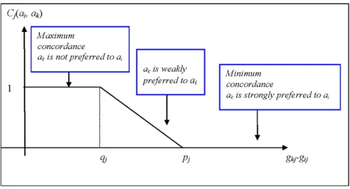
Cj(ai, ak) =      1 if gkj ≤ gij + qj 0 if gkj ≥ gij+ pj gij−gkj+pj pj−qj otherwise (3)

where qj and pj are the indifference and the preference thresholds associated to critj. If

gkj ≥ gij+pj, then the DM prefers the alternative akto the alternative ai(strict preference);

Figure 1: Local concordance index Cj(ai, ak)

since the alternative aiis dominated by the alternative ak. On the contrary if gkj ≤ gij+ qj,

then the alternative ak is not preferred to ai, and this implies that the local concordance

index of (ai, ak) reaches its maximum value. In the intermediate preference region, where

the decision maker is not sure if he prefers akor ai (weak preference), the local concordance

index takes values in the interval (0,1). Figure 1 may be illustrative.

Similarly to the local concordance, for each pair of alternatives (ai, ak) and for each

criterion critj, the method computes the discordance index Dj(ai, ak) which indicates the

discordance of the hypothesis that ai dominates ak according to critj. The discordance

index is constructed as follows:

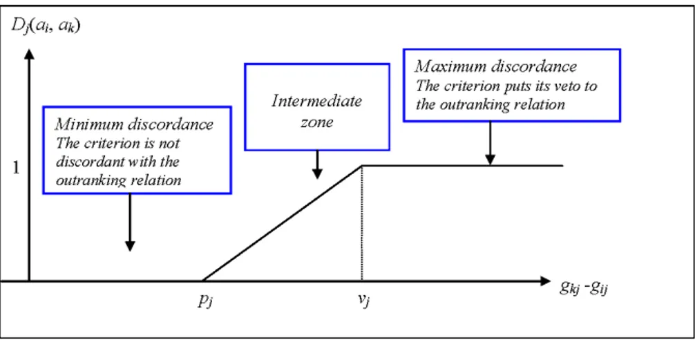
Dj(ai, ak) =      0 if gkj ≤ gij+ pj 1 if gkj ≥ gij + vj gkj−gij−pj vj−pj otherwise (4)

where vj is a veto threshold (with vj ≥ pj) that is used to reject the hypothesis that the

alternative ai is at least as good as the alternative ak if gkj ≥ gij + vj; in this case the

discordance index reaches its maximum value (see figure 2). As one can better see later, the veto threshold allows to treat the situation in which an alternative with a bad performance in a given critical criterion will receive a bad final score.

The local discordance index is instead minimal when the criterion critj is not discordant

with the statement that the alternative aioutranks (is at least as good as) the alternative ak.

On the intermediate zone, it is assumed that the discordance index increases in proportion to the difference gkj− gij.

The indexes (3) and (4) are computed for each pair of alternatives (ai, ak) and for each

criterion critj. As a final result of the first phase, both local concordance and discordance

are used in order to obtain an index that indicates how much the alternative ai outranks

Figure 2: Local discordance index Dj(ai, ak)

alternatives (ai, ak) is computed as follows:

O(ai, ak) = ( C(ai, ak) if Dj(ai, ak) ≤ C(ai, ak) ∀j C(ai, ak)Qj∈T 1−Dj(ai,ak) 1−C(ai,ak) otherwise (5) where C(ai, ak) represents the aggregation of the local concordance indexes, obtained as the

weighted arithmetic mean of the local concordance indexes (3), with normalized weights wj

indicating the relative importance of each criterion critj(j = 1, ..., n), that is:

C(ai, ak) = n

X

j=1

wjCj(ai, ak) (6)

We observe that the outranking index coincides with the aggregate concordance if C(ai, ak) is greater than the discordance indexes Dj(ai, ak), for all criteria. Otherwise,

if there exist one or more criteria for which the discordance exceeds the aggregate concor-dance, then the score is reduced. More precisely, let T denote the subset of criteria for which Dj(ai, ak) > C(ai, ak); then the outranking index is equal to

C(ai, ak) Y j∈T 1 − Dj(ai, ak) 1 − C(ai, ak) (7) this means that C(ai, ak) is multiplied by as many factors (less than one) as there are the

criteria belonging to T . Moreover, if there exists even only one criterion critj for which

there is maximum discordance (i.e. Dj(ai, ak) = 1) then the outranking index is equal to

zero. This entails that if for a given criterion the alternative ai is so much worse than the

alternative ak, then one cannot consider ai at least as good as ak, even this is true for all

Phase II

The outranking index (5) is used in this phase in order to obtain a ranking of the alternatives. Following the methodology of PROMETHEE II, for each alternative ai, a

leaving flow ϕ+_(a

i) and an entering flow ϕ−(ai) are computed as follows:

ϕ+(ai) = X k6=i O(ai, ak) (8) ϕ−(ai) = X k6=i O(ak, ai) (9)

which indicate respectively the strength of ai over the remaining alternatives and the

weak-ness of ai over the other ones. Then, in order to obtain a total preorder of the alternatives,

and not only partial ones (see [12]), an index (a net flow) is computed as the difference between the leaving and the entering flow:

ϕ(ai) = ϕ+(ai) − ϕ−(ai) (10)

so that the alternatives can be rank, in a descending order, according to the net flow (10).

2.2 PSO application to preference disaggregation

The determination of the parameters of the model can be performed using direct or indirect procedures. The former requires that the DM explicitly determines the parameters that express its preference structure, while the latter pick out the parameters using preference disaggregation methods based on a sample reference set of decisions (see [13] and [9]). In this case, a mathematical programming problem has to be solved to infer the parameters so that the model obtained is as much as possible consistent with the ordering of the reference set provided by the DM. Because of the size and the complexity of the problem considered, in this paper we use an evolutionary methodology, Particle Swarm Optimization (PSO), as an algorithm for the numerical solution of the mathematical programming problem involved. Other metaheuristics approaches to similar problems can be found in [9] and [1].

In the following of this section we will present the formulation of the optimization problem associated to the preference disaggregation problem and the evolutionary approach for the determination of the parameters of the MURAME model.

2.2.1 Mathematical formulation of preference disaggregation method

As we have seen in section 2.1, in order to apply the described MURAME-based model and to rank the alternatives, we have to determine the following parameters:

• the vector of the weights: w = (w1, . . . , wn), with wj ≥ 0, j = 1, . . . , n andPjwj = 1;

• the vector of indifference thresholds: q = (q1, . . . , qn), with qj ≥ 0, j = 1, . . . , n;

• the vector of veto thresholds: v = (v1, . . . , vn), with vj ≥ pj, j= 1, . . . , n.

Let us suppose to have a reference set of decisions of the DM, that is a set of past decisions regarding the alternatives, or regarding a subset A′ _{⊆ A of the whole set of the}

alternatives.

Given the ordering of the alternatives in the reference set made by the DM, the preference disaggregation approach regards the problem of determining the set of parameters that minimizes a measure of inconsistency f (w, q, p, v) between the ordering produced by the model with that set of parameters and the given one. In order to infer the values of the parameters starting from a given reference set of decisions of the DM, the following mathematical programming problem has to be solved:

min w,q,p,v f(w, q, p, v) s.t. w ≥ 0 n X j=1 wj = 1 q≥ 0 p≥ q v≥ p . (11)

We can note that problem (11) can be reformulated in a simpler way by introducing the auxiliary variables t = p − q and s = v − p, so that it becomes:

min w,q,t,s f(w, q, t, s) s.t. w, q, t, s ≥ 0 n X j=1 wj = 1 . (12)

This apparently simple mathematical programming problems hides its complexity in the objective function f (w, q, t, s): indeed every choice of f requires that it produces an order of the alternatives and then that a measure of the consistency of the model is calcu-lated. It is then hard to write an exact analytical expression for f in term of its variables w, q, t, s, so that the use of gradient methods for the optimization task is discouraged, and an evolutionary approach seems more appropriate.

In this study we consider two kinds of fitness function, in order to exploit all the infor-mation contained in the input data provided by the DM1: the first function allows to deal with the ordinal rank of the alternatives in the reference set, whereas the second one allows to handle the cardinal values.

The first fitness function is the S function defined as follows: S(w, q, t, s) = 6

Pm′

i=1(¯ri− ri(w, q, t, s))2

m′3_{− m}′ (13)

1

where ¯riis the rank of alternative aiin the reference set assigned by the DM and ri(w, q, t, s)

the one determined by the MURAME-based model, with m′ ≤ m being the total number of alternatives in the reference set. This fitness function is an application of the Spearman Rank Correlation Coefficient (see [15]) to measure the strength of correlation between the two orderings; its values are in the interval [0, 2], and S(w, q, t, s) = 0 clearly means that there is an exact correspondence between the ranking of the DM and that obtained by the model.

The second fitness function is represented by the following D function: D(w, q, t, s) =

Pm′

i=1(λ(ϕ(ai; w, q, t, s)) − s(ai))2

m′ (14)

where s(ai) is the (cardinal) score assigned by the DM to the alternative ai and λ is a linear

transformation that maps the net flow ϕ(ai; w, q, t, s) (10) produced by the model to the

support of DM scores.

2.2.2 PSO implementation

Particle Swarm Optimization is a bio-inspired iterative heuristics for the solution of non-linear global optimization problems (see [2], [14]). The basic idea of PSO is to model the so called “swarm intelligence” ([3]) that drives groups of individuals belonging to the same species when they move all together looking for food. On this purpose every member of the swarm explores the search area keeping memory of its best position reached so far, and it exchanges this information with the neighbors in the swarm. Thus, the whole swarm is supposed to converge eventually to the best global position reached by the swarm members. From a mathematical point of view every member of the swarm (namely a particle) represents a possible solution of an optimization problem, and it is initially positioned randomly in the feasible set of the problem. To every particle is also initially assigned a random velocity, which is used to determine its initial direction of movement.

For a more formal description of PSO, let us consider the following global optimization problem:

min

x∈Rdf(x),

where f : Rd _{7→ R is the objective function in the minimization problem. In applying}

PSO for its solution, we consider M particles; at the k-th step of the PSO algorithm, three vectors are associated to each particle l ∈ {1, . . . , M }:

• xk

l ∈ Rd, the position at step k of particle l;

• vk

l ∈ Rd, the velocity at step k of particle l;

• pl∈ Rd, the best position visited so far by the l-th particle.

Moreover, pbestl = f (pl) denotes the value of the objective function in the position pl of

the l-th particle.

1. Set k = 1 and evaluate f (xk

l) for l = 1, . . . , M . Set pbestl= +∞ for l = 1, . . . , M .

2. If f (xk

l) < pbestl then set pl= xkl and pbestl= f (xkl).

3. Update position and velocity of the l-th particle, with l = 1, . . . , M , according to the following equations: vk+1_l = wk+1vk_l + Uφ1 ⊗ (pl− x k l) + Uφ2 ⊗ (pg(l)− x k l) (15) xk+1_l = xk_l + vk+1_l (16) where Uφ1, Uφ2 ∈ R

d _{and their components are uniformly randomly distributed in}

[0, φ1] and [0, φ2] respectively; parameters φ1 and φ2 are often called acceleration

co-efficients; the symbol ⊗ denotes component-wise product and p_g(l)is the best position in a neighborhood of the l-th particle.

The parameter wk_{(the inertia weight) is generally linearly decreasing with the number}

of steps, i.e.:

wk = wmax+

wmin− wmax

K k,

where K is the maximum number of steps allowed.

4. If a convergence test is not satisfied then set k = k + 1 and go to 2.

For more details about PSO methodology, the specification of its parameters and of the neighborhood topology, we refer the reader to [2]. In our implementation we have considered the so called gbest topology, that is g(l) = g for every l = 1, . . . , M , and g is the index of the best particle in the whole swarm, that is g = arg min_l=1,...,Mf(pl). This choice implies

that the whole swarm is used as the neighborhood of each particle. Moreover, as stopping criterion, we decided that the algorithm terminated when the objective function didn’t have a decrease of at least 10−4 _{in a prefixed number of steps.}

Since PSO was conceived for unconstrained problems, the algorithm above cannot pre-vent from generating infeasible particles’ positions when constraints are considered. To avoid this problem, different strategies have been proposed in the literature, and most of them involve the repositioning of the particles ([22]) or the introduction of some external criteria to rearrange the components of the particles ([8] and [20]). In this paper we fol-low the same approach adopted in [6], which consists in keeping PSO as in its original formulation and reformulating the optimization problem into an unconstrained one:

min

where the objective function P (w, q, t, s; ε) is defined as follows: P(w, q, t, s; ε) = f (w, q, t, s) + 1 ε "      n X j=1 wj− 1       + n X j=1 max{0, −wj} + n X j=1 max{0, −qj} + n X j=1 max{0, −tj} + n X j=1 max{0, −sj} # (18)

with ε being the penalty parameter. The approach adopted is called ℓ1 penalty function

method; for more details about this method and about the relationships between the so-lutions of the constrained problem (12) and those of the unconstrained problem (17), see [21, 11] and [17, 6].

We may observe that the penalty function P (w, q, t, s; ε) is clearly nondifferentiable because of the ℓ1-norm in (18); this feature contributes to motivate the choice of using

PSO, since it does not require the derivatives of P (w, q, t, s; ε). However, since PSO is a heuristics, the minimization of the penalty function P (w, q, t, s; ε) does not theoretically ensure that a global minimum of problem (12) is detected. Nevertheless, PSO often provides a suitable compromise between the performance of the approach (i.e. a satisfactory estimate of the global minimum solution for problem (12)) and its computational cost.

With regard to the initialization procedure, we can observe that, since we deal with an unconstrained problem, we could in principle generate initial values for the population in an arbitrary random way. However, like any metaheuristic, the performance of the algorithm could be improved by a careful choice of the initial population such that the feasible region is adequately explored by the particles at the initial step.

In this contribution, in order to obtain the initial weights, we generated d1<· · · < dn−1

random numbers uniformly distributed in [0, 1], and then we set: w₁0= d1, w02 = d2− d1, . . . , w0n= 1 − dn−1.

To obtain the initial values of the variables qj, tj, sj (j = 1, . . . , n), we generated three

random numbers a1

j < a2j < a3j uniformly distributed in [0, 2], and then we set:

q0_j = (g_j − g_j)a 1 j 10 t0_j = (g_j − g_j)a 2 j 10 s0_j = (g_j − g_j)a 3 j 10

where g_j = max1≤i≤mgij and g_j = min1≤i≤mgij.

Moreover, for every particle x0_l = (w_l0, q0_l, t0_l, s0_l), the components of the initial velocity v0_l are generated as random numbers uniformly distributed in [−x0_h, x0_h] for every h = 1, . . . , 4n.

3

Application to a creditworthiness evaluation problem

In this section we analyze the performance of the proposed approach by considering a credit scoring problem. We adopt the MURAME method in order to evaluate the creditworthiness of a set of firms, as proposed in [7], and use a real world data set provided by a major bank of north-eastern Italy, the Banca Popolare di Vicenza2.

The database consists of around 12 000 firms applicants for a loan, which represent the alternatives of the creditworthiness evaluation problem. The firms are divided into three groups, small, medium and large, with respect to their business turnover and the three groups are approximately of the same size. The evaluation criteria are represented by seven indicators {I1, ..., I7} which have been computed by the bank starting from the balance

sheets; their values are provided for both years 2008 and 2009. As reference decisions, we considered the final scores that the bank assigned to the firms in order to establish their ranking in terms of their credit quality.

The main goal of our analysis is to verify if PSO is able to find, using a realistic com-putational time, the values of the parameters of the MURAME model that make them consistent with the actual classification of the firms provided by the bank, which acts as the decision maker.

The experimental analysis has been conducted in two phases, similarly to [9].

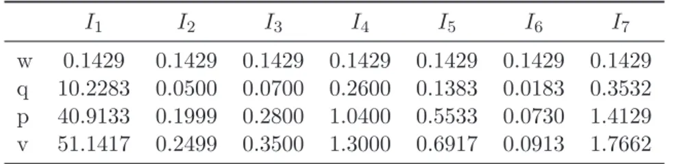
In the first phase we consider a subset of randomly selected 4000 firms. In order to test both the training than the predictive performance, we employ a bootstrap analysis. Using data of year 2008, the firms have been ordered using the MURAME methodology and the values of the parameters have been fixed according to the following specific rules, as proposed in [7]: w1 = · · · = wn= 1 n, qj = (gj − gj) 1 6, pj = 4qj, vj = 5qj j= 1, . . . , n. (19) Table 1 reports the values of the parameters so obtained, which will be a reference point for our subsequent analysis.

I1 I2 I3 I4 I5 I6 I7

w 0.1429 0.1429 0.1429 0.1429 0.1429 0.1429 0.1429 q 10.2283 0.0500 0.0700 0.2600 0.1383 0.0183 0.3532 p 40.9133 0.1999 0.2800 1.0400 0.5533 0.0730 1.4129 v 51.1417 0.2499 0.3500 1.3000 0.6917 0.0913 1.7662

Table 1: Actual parameters of MURAME

A first set of bootstrap experiments has been first conducted in order to determine the best values for the acceleration coefficients φ1, φ2, the maximum number of steps K and the

value of the penalty parameter ε, while for the initial and final value of the inertia weight we used the ones most used in the literature. In these experiments we have considered

2

only the training step (see beyond) and we have used as fitness function S+D₂ , with several combinations of values for the PSO parameters. The PSO parameters have been chosen as the combination of values that allowed to obtain on average the best results for the objective function. Table 2 reports the values of the PSO parameters so obtained.

φ1 φ2 K ε wmin wmax

1.75 1.75 200 0.0001 0.4 0.9 Table 2: PSO parameters

The bootstrap procedure that we have adopted is structured in the following steps. (i) A sample of H = 100 firms is randomly selected without replacement from the 4000

ones.

(ii) To the sample of firms selected as in step (i) we have applied the MURAME method-ology with the actual parameters determined as in table 1; an ordering of the H firms is obtained according to the net flow (10) associated to each firm.

(iii) To the sample of firms selected as in step (i) we have applied the PSO-based method-ology, using the PSO parameters determined as in table 2 and adopting both objective functions (13), (14). The optimal values of MURAME parameters are therefore deter-mined through PSO, in order to minimize the discrepancy–as measured by the fitness function– between the score (ranking) obtained by the MURAME in step (ii) and that one computed by PSO (the so-called training step).

(iv) (Out-the-bootstrap). Another sample of firms of the same size H = 100 is randomly selected from the 4000 ones, excluding those belonging to the sample used for the training step. This sample is ordered with the MURAME method, by using both the actual MURAME parameters and those determined by PSO; the value of the fitness function is then computed in order to evaluate the distance between the two orderings. The procedure is then repeated N = 1000 times in order to compute the necessary statistics of the values of the MURAME parameters and the performance measures. Table 3 reports the average (and the standard deviation) of the fitness function values obtained at each iteration of the procedure. The results are shown for both the fitness functions S and D and for a population size of M = 100 and M = 200 number of particles. Table 4 presents the results obtained for the out-the-bootstrap phase.

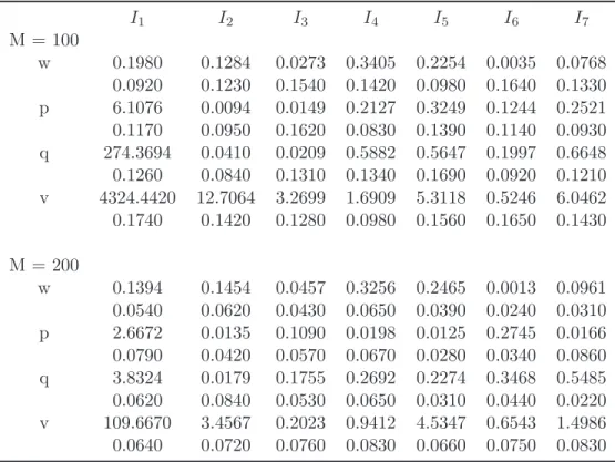
It can be noted that while M = 100 particles are enough to obtain full consistency (an average value of the fitness function nearly zero), with both the performance measures considered, between the model produced by PSO and the actual ordering of the alternatives in the bootstrap data, the performance of the so obtained models on the out of the bootstrap data is not as good, and a higher number of particles (M = 200) is required to improve it. Table 5 illustrates the average values of the parameters (and the standard deviations) determined by PSO in the bootstrap procedure.

M=100 M=200

S D S D

Mean 0.0022 0.0025 0.0002 0.0003 Standard deviation 0.0011 0.0017 0.0001 0.0002

Table 3: Results for in-the-bootstrap data

M=100 M=200

S D S D

Mean 0.1234 0.1725 0.012 0.016 Standard deviation 0.0450 0.0612 0.032 0.035

Table 4: Results for out-the-bootstrap data

I1 I2 I3 I4 I5 I6 I7 M = 100 w 0.1980 0.1284 0.0273 0.3405 0.2254 0.0035 0.0768 0.0920 0.1230 0.1540 0.1420 0.0980 0.1640 0.1330 p 6.1076 0.0094 0.0149 0.2127 0.3249 0.1244 0.2521 0.1170 0.0950 0.1620 0.0830 0.1390 0.1140 0.0930 q 274.3694 0.0410 0.0209 0.5882 0.5647 0.1997 0.6648 0.1260 0.0840 0.1310 0.1340 0.1690 0.0920 0.1210 v 4324.4420 12.7064 3.2699 1.6909 5.3118 0.5246 6.0462 0.1740 0.1420 0.1280 0.0980 0.1560 0.1650 0.1430 M = 200 w 0.1394 0.1454 0.0457 0.3256 0.2465 0.0013 0.0961 0.0540 0.0620 0.0430 0.0650 0.0390 0.0240 0.0310 p 2.6672 0.0135 0.1090 0.0198 0.0125 0.2745 0.0166 0.0790 0.0420 0.0570 0.0670 0.0280 0.0340 0.0860 q 3.8324 0.0179 0.1755 0.2692 0.2274 0.3468 0.5485 0.0620 0.0840 0.0530 0.0650 0.0310 0.0440 0.0220 v 109.6670 3.4567 0.2023 0.9412 4.5347 0.6543 1.4986 0.0640 0.0720 0.0760 0.0830 0.0660 0.0750 0.0830

Table 5: Average values (and standard deviation) of MURAME parameters, determined by bootstrap procedure

It is interesting to remark that the discrepancies between the values of the parameters obtained with M = 100 and M = 200 are not very high and they concern mainly the values of the thresholds, while the weights are determined in a consistent way even with the smaller number of particles.

As for the relation between the actual parameters of table 1 and the average values of parameters obtained in table 5, it can be noticed that there are significant differences, similarly to what observed in [9] with regard to the use of the differential evolution algorithm. However, since the ordering performance of the model is high, this seems to suggest that there is a certain flexibility in the specification of the parameters of the model consistent with the ordering of the alternatives in the reference set.

In the second phase of our analysis we aimed at determining the parameters of the preference structure of the DM (the bank) for both 2008 and 2009 years. The objective of this second phase was to determine if the PSO procedure was able to determine, starting from the reference set and using a reasonable computational time, a MURAME model that was consistent with the ordering of firms provided by the bank.

As validation set we considered the whole set of firms, for year 2009, in each of the three groups, small, medium and large firms (each group is made up of around 4000 firms). As reference set we used two subsets of m′ _{= 100 and m}′ _{= 500 firms respectively, keeping}

the number of particles fixed at M = 200, with data of year 2008. In this way we analyze the impact of the higher size of the reference and validation set on the number of particles required to achieve a good quality of the model produced.

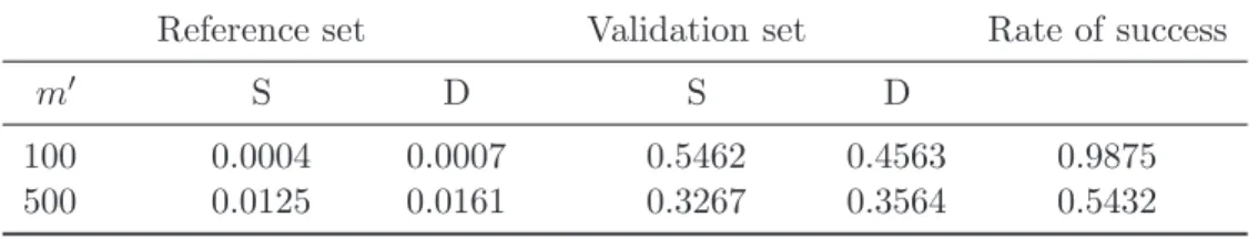
In table 6 we present the results obtained for the analysis connected to the small firms; there are indeed no important differences between the results obtained for the three groups of firms considered, and this is quite evident since the firms are ordered by the bank using the same procedure.

Reference set Validation set Rate of success

m′ _{S D S D}

100 0.0004 0.0007 0.5462 0.4563 0.9875

500 0.0125 0.0161 0.3267 0.3564 0.5432

Table 6: Results obtained for the real world problem, in case of the small firms In the columns entitled Reference set, table 6 illustrates the average (over 20 runs of the algorithm) of the fitness function values computed by comparing the ranking obtained by PSO on the sample of firms used as reference set (100 and 500 firms, respectively) and the ranking provided by the bank. The results are presented for both the fitness functions S and D. In the columns entitled Validation set, the table illustrates the average value of the fitness function computed by comparing the ranking obtained by PSO on the whole set of small firms (around 4000 firms) and the ranking provided by the bank. The last column shows the rate of success, that is the ratio between the successful runs of the algorithm (i.e. the runs for which the optimal value S = D = 0 is achieved within the maximum number of steps allowed) and the total number of runs.

It appears clearly that for such a large size of the validation set, a greater reference set is needed to achieve a satisfactory consistence with the actual ordering. However, with a greater reference set, the capability of the algorithm to find an optimal solution decreases, as the rate of success shows.

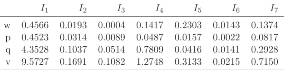
Finally, in table 7 we show the average values of the optimal parameters obtained in the case of m′ _{= 500 firms as reference set. It is interesting to have a look at the weights}

of the criteria: it emerges clearly that indicators I2, I3 and I6 play a marginal role in

the implicit preference structure expressed by the bank. While for indicator I2, as it is

shown in table 8, this behaviour can be a priori explained by its high correlation with indicator I4, we don’t have a such evident interpretation for indicators I3 and I6 and a

financial interpretation is not possible in this analysis, due to the nature of the indicators considered that have been computed directly by the bank from the balance sheet, but that are provided us without giving their formal description. Anyway, it is important to note that this additional information we have obtained, could be used by the decision maker to improve or refine its internal credit modeling policy.

I₁ I₂ I₃ I₄ I₅ I₆ I₇

w 0.4566 0.0193 0.0004 0.1417 0.2303 0.0143 0.1374 p 0.4523 0.0314 0.0089 0.0487 0.0157 0.0022 0.0817 q 4.3528 0.1037 0.0514 0.7809 0.0416 0.0141 0.2928 v 9.5727 0.1691 0.1082 1.2748 0.3133 0.0215 0.7150

Table 7: Average values of the parameters obtained for the real world problem, in case of the small firms

I₁ I₂ I₃ I₄ I₅ I₆ I₇ I1 1.0000 I2 0.3134 1.0000 I3 0.3602 0.2751 1.0000 I4 0.4157 0.6562 0.1796 1.0000 I5 0.2758 0.2493 0.2219 0.2394 1.0000 I₆ 0.4926 0.3766 0.2680 0.2980 0.2184 1.0000 I7 -0.0025 0.1146 0.1370 -0.0650 -0.0221 0.0683 1.0000

4

Final remarks

The novelty of this contribution consists in dealing with the problem of preference disag-gregation in a MURAME context. To tackle this problem, we adopted an evolutionary algorithm based on the Particle Swarm Optimization (PSO) method and tested the ap-proach proposed on a credit scoring problem, using real data.

Since MURAME determines the outranking index with respect to each other alterna-tive in the reference set, the computational effort required is notably higher than other multicriteria models, for example the ELECTRE TRI based models which consider only the reference profiles (see [16]).

The results obtained in this contribution showed a high consistency between the model produced by PSO and the actual ordering of the alternatives.

The machine time depends on the numerousness of the reference set and on that of the validation set; for example, in the bootstrap phase, with a reference set of 100 firms, 7 minutes are needed in order to make 200 steps of the PSO (and this means 7000 minutes in order to carry out the 1000 runs of the bootstrap analysis). In the case of a reference set of 500 firms the time machine is higher, almost 3 hours to implement 200 steps of the algorithm3.

As future research we intend to find the way of reducing the machine time, by conve-niently simplifying the process according to which the model compares each pair of alter-natives, for example by permitting a mere comparison with some reference profiles.

References

[1] N. Belacel, H. Bhasker Raval, and A. P. Punnen. Learning multicriteria fuzzy classifi-cation method PROAFTN from data. Computers & Operations Research, 34(7):1885 – 1898, 2007.

[2] T. Blackwell, J. Kennedy, and R. Poli. Particle swarm optimization - an overview. Swarm Intelligence, 1(1):33 – 57, 2007.

[3] E. Bonabeau, M. Dorigo, and G. Theraulaz. From Natural to Artificial Swarm Intelli-gence. Oxford University Press, 1999.

[4] J. P. Brans and Ph. Vincke. A preference ranking organisation method: (the PROMETHEE method for multiple criteria decision-making). Management Science, 31(6):647 – 656, 1985.

[5] J. Buchanan, P. Sheppard, and D. Vanderpooten. Project ranking using ELECTRE III. Research report 99-01, University of Waikato, Dept of Management Systems, New-Zealand, 1999.

3

[6] M. Corazza, G. Fasano, and R. Gusso. Portfolio selection with an alternative measure of risk: Computational performances of particle swarm optimization and genetic algo-rithms. In C. Perna and M. Sibillo, editors, Mathematical and Statistical Methods for Actuarial Sciences and Finance, pages 123–130. Springer, 2012.

[7] M. Corazza, S. Funari, and F. Siviero. An MCDA-based approach for creditworthiness assessment. Working Papers 177, Department of Applied Mathematics, University of Venice, November 2008.

[8] T. Cura. Particle swarm optimization approach to portfolio optimization. Nonlinear Analysis: Real World Applications, 10(4):2396 – 2406, 2009.

[9] M. Doumpos, Y. Marinakis, M. Marinaki, and C. Zopounidis. An evolutionary ap-proach to construction of outranking models for multicriteria classification: The case of the electre tri method. European Journal of Operational Research, 199(2):496 – 505, 2009.

[10] M. Doumpos and C. Zopounidis. Preference disaggregation and statistical learning for multicriteria decision support: A review. European Journal of Operational Research, 209(3):203 – 214, 2011.

[11] R. Fletcher. Practical methods of optimization. John Wiley & Sons, Glichester, 1991. [12] Y. Goletsis, D. T. Askounis, and J. Psarras. Multicriteria judgments for project rank-ing: An integrated methodology. Economic Financial Modelling, pages 127 – 148, Autumn Issue 2001.

[13] E. Jacquet-Lagrze and Y. Siskos. Preference disaggregation: 20 years of MCDA expe-rience. European Journal of Operational Research, 130(2):233 – 245, 2001.

[14] J. Kennedy and R. C. Eberhart. Particle swarm optimization. Proceedings of the IEEE international conference on neural networks IV, pages 1942 – 1948, 1995.

[15] E.L. Lehmann and H.J.M. D’Abrera. Nonparametrics: statistical methods based on ranks. Prentice Hall, 1998.

[16] V. Mousseau, R. Slowinski, and P. Zielniewicz. ELECTRE TRI 2.0a: Methodological guide and user’s documentation. Universit de Paris-Dauphine, 1999.

[17] G. Di Pillo and L. Grippo. Exact penalty functions in constrained optimization. SIAM Journal on Control and Optimization, 27(6):1333 – 1360, 1989.

[18] B. Roy. ELECTRE III: Un algorithme de classements fond sur une representation floue des prfrences en prsence de critres multiples. Cahiers du CERO, 20(1):3 – 24, 1978. [19] Y. Shi and R. Eberhart. A modified particle swarm optimizer. In Evolutionary

Compu-tation Proceedings, 1998. IEEE World Congress on CompuCompu-tational Intelligence., The 1998 IEEE International Conference on, pages 69 – 73, 1998.

[20] N. Thomaidis, T. Angelidis, V. Vassiliadis, and G. Dounias. Active portfolio manage-ment with cardinality constraints: An application of particle swarm optimization. New Mathematics and Natural Computation, 5(3):535 – 555, 2009.

[21] W. I. Zangwill. Non-linear programming via penalty functions. Management Science, 13(5):344 – 358, 1967.

[22] W.J. Zhang, X. F. Xie, and D. C. Bi. Handling boundary constraints for numerical optimization by particle swarm flying in periodic search space. In Proceedings of the 2004 Congress on Evolutionary Computation IEEE, pages 2307 – 2311, 2005.