Anton Frisk Kockum
1, Vincenzo Macrì
1,2, Luigi Garziano
1,2,3, Salvatore Savasta
1,2&
Franco Nori
1,4We propose a new method for frequency conversion of photons which is both versatile and deterministic. We show that a system with two resonators ultrastrongly coupled to a single qubit can be used to realise both single- and multiphoton frequency-conversion processes. The conversion can be exquisitely controlled by tuning the qubit frequency to bring the desired frequency-conversion transitions on or off resonance. Considering recent experimental advances in ultrastrong coupling for circuit QED and other systems, we believe that our scheme can be implemented using available technology.
Frequency conversion in quantum systems1, 2, is important for many quantum technologies. The optimal work-ing points of devices for transmission, detection, storage, and processwork-ing of quantum states are spread across a wide spectrum of frequencies3, 4. Interfacing the best of these devices is necessary to create quantum networks5 and other powerful combinations of quantum hardware. Examples of frequency-conversion setups developed for such purposes include upconversion for photon detection6 and storage7, since both these things are easier to achieve at a higher frequency than what is optimal for telecommunications. Downconversion in this frequency range has also been demonstrated8–10, and recently even strong coupling between a telecom and a visible optical mode11. Additionally, advances in quantum information processing with superconducting circuits at microwave frequencies12, 13, is driving progress on frequency conversion between optical and microwave frequencies14–17. We note that several types of quantum systems, suited for different tasks in quantum information processing, can operate at microwave frequencies4. To connect these systems, frequency conversion within this frequency range is important. Furthermore, frequency conversion can be used to create entangled states, which have applications in virtually all areas of quantum information processing, including quantum computing, quantum key distribution, and quantum teleportation18.
Circuit quantum electrodynamics (QED)12, 19–22, offers a wealth of possibilities for frequency conversion at microwave frequencies; some of these schemes can also be generalised to optical frequencies. By modulating the magnetic flux through a superconducting quantum interference device (SQUID) in a transmission-line resonator, the frequency of the photons in the resonator can be changed rapidly23–25, or two modes of the resonator can be coupled26, 27. Other driven Josephson-junction-based devices can also be used for microwave frequency conver-sion28, 29. Downconversion has been proposed for setups with Δ-type three-level atoms30–32, and demonstrated with an effective three-level Λ system33. Upconversion of a two-photon drive has been shown for a flux qubit coupled to a resonator in a way that breaks parity symmetry34. Indeed, the Δ-type level structure in a flux qutrit35 even makes possible general three-wave mixing36. Recently, frequency conversion was also demonstrated for two sideband-driven microwave LC-resonators coupled through a mechanical resonator37.
The approach to frequency conversion that we propose in this article is based on two cavities or resonator modes coupled ultrastrongly to a two-level atom (qubit). The regime of ultrastrong coupling (USC), where the coupling strength starts to become comparable to the bare transition frequencies in the system, has only recently been reached in a number of solid-state systems38–56. Among these, a few circuit-QED experiments provide some of the clearest examples39, 40, 49–52, 54–56, including the largest coupling strength reported51. While the USC regime displays many striking physical phenomena57–66, we are here only concerned with the fact that it enables higher-order processes that do not conserve the number of excitations in the system, an effect which has also been noted for a multilevel atom coupled to a resonator67. Examples of such processes include multiphoton Rabi oscil-lations68, 69, and a single photon exciting multiple atoms70. Indeed, almost any analogue of processes from non-linear optics is feasible71; this can be regarded as an example of quantum simulation72, 73. Just like the analytical
1Center for Emergent Matter Science, Riken, Saitama, 351-0198, Japan. 2Dipartimento di Scienze Matematiche e Informatiche, Scienze Fisiche e Scienze della Terra, Università di Messina, I-98166, Messina, Italy. 3School of Physics and Astronomy, University of Southampton, Southampton, SO17 1BJ, United Kingdom. 4Physics Department, The University of Michigan, Ann Arbor, Michigan, 48109-1040, USA. Correspondence and requests for materials should be addressed to A.F.K. (email: [email protected])
Received: 15 February 2017 Accepted: 10 May 2017 Published: xx xx xxxx
solution for the quantum Rabi model74 is now being extended to multiple qubits75, 76, and multiple resonators77–79, we here extend the exploration of non-excitation-conserving processes to multiple resonators.
In our proposal, the qubit frequency is tuned to make various frequency-converting transitions resonant. For example, making the energy of a single photon in the first resonator equal to the sum of the qubit energy and the energy of a photon in the second resonator enables the conversion of the former (a high-energy photon) into the latter (a low-energy photon plus a qubit excitation) and vice versa. In the same way, a single photon in the first resonator can be converted into multiple photons in the second resonator (and vice versa) if the qubit energy is tuned to make such a transition resonant. The proposed frequency-conversion scheme is deterministic and allows for a variety of different frequency-conversion processes in the same setup. The setup should be possible to imple-ment in state-of-the-art circuit QED, but the idea also applies to other cavity-QED systems.
We note that the process of parametric down-conversion in this type of circuit-QED setup has been consid-ered previously80, but in a regime of weaker coupling and without using the qubit to control the process. Also, it has been shown that a beamsplitter-type coupling between two resonators can be controlled by changing the qubit state81 or induced for weaker qubit-resonator coupling by driving the qubit82, but the proposal presented here offers greater versatility and simplicity for frequency conversion.
Model
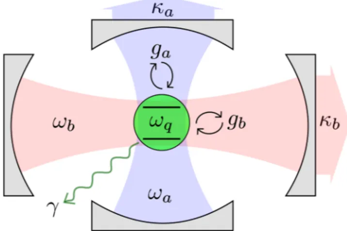
We consider a setup where a qubit with transition frequency ωq is coupled to two resonators with resonance
fre-quencies ωa and ωb, respectively, as sketched in Fig. 1. The Hamiltonian is (ħ = 1)
ω ω ω σ σ θ σ θ = + + + + + + + ˆ ˆ ˆ† ˆ ˆ† ˆ ˆ ˆ† ˆ ˆ† ˆ ˆ H a a b b g a a g b b 2 [ ( ) ( )]( cos sin ), (1) a b q z a b x z
where ga (gb) denotes the strength of the coupling between the qubit and the first (second) resonator. The creation
and annihilation operators for photons in the first (second) resonator are ˆa and ˆa (ˆb and ˆ† b ), respectively. The †
angle θ parameterises the amount of longitudinal and transverse coupling as, for example, in experiments with flux qubits34, 39, 40, 49, 56, 83; σˆ
x and σˆz are Pauli matrices for the qubit.
Note that we do not include a direct coupling between the two resonators. Such a coupling is seen in exper-iments49, but here we will only be concerned with situations where the resonators are far detuned from each other, meaning that this coupling term can safely be neglected. Likewise, we do not include higher modes of the resonators. While they may contribute in experiments with cavities and transmission-line resonators, they can be avoided by using lumped-element resonators56, 84.
The crucial feature of Eq. (1) for our frequency-conversion scheme is that some of the coupling terms do not conserve the number of excitations in the system. The σˆz coupling terms act to change the photon number in one
of the resonators by one, while keeping the number of qubit excitations unchanged. Likewise, the σˆx coupling
contains terms like σa and σˆ ˆ− b that change the number of excitations in the system by two. For weak coupling ˆ ˆ†+
strengths, all such terms can be neglected using the rotating-wave approximation (RWA), but in the USC regime the higher-order processes that these terms enable can become important and function as second- or third-order nonlinearities in nonlinear optics71.
To include the effect of decoherence in our system, we use a master equation on the Lindblad form in our numerical simulations. The master equation reads
∑
ρ= − ρ + Γ + Γ + Γ ρ > ˆ i H[ , ]ˆ ˆ(
)
[j k] ,ˆ (2) j k j a jk bjk qjk ,Figure 1. A sketch of the system. A qubit (green) is coupled to two resonator modes (blue, a, and red, b). Decoherence channels for the qubit (relaxation rate γ) and the resonators (relaxation rates κa, κb) are included.
where ρˆ is the density matrix of the system, [ ]cˆρ=c cˆ ˆˆρ †− 1ρˆˆ ˆc c† − c cˆ ˆ ˆ†ρ
2 21
, and the states in the sum are
eigen-states of the USC system. The relaxation rates are given by Γ =ajk κa Xajk 2, Γ =bjk κb Xbjk 2, and Γ =qjk γCjk 2,
where κa, κb, and γ are the relaxation rates for the bare states of the resonators and the qubit, respectively, and
= ˆ
cjk j c k with = +Xˆ aˆ aˆ†
a , = +Xˆb bˆ bˆ†, and Cˆ=σˆx85, 86, Writing the master equation in the eigenbasis of
the full system avoids unphysical effects, such as emission of photons from the ground state. Similarly, to correctly count the number of photonic and qubit excitations we use X Xˆ ˆa− +a ,
− +
ˆ ˆ X Xb b , and
− +
ˆ ˆ
C C , where the plus and minus signs denote the positive and negative frequency parts, respectively, of the operators in the system eigen-basis, instead of a a , 〈ˆ ˆ† b b , and σ σˆ ˆ† 〉
+ −
ˆ ˆ 86.
In the simulations presented in the next section, we use parameters that can be reached in circuit-QED exper-iments. In such experiments, the bare transition frequencies are usually in the range ωa/b/q ~ 2π × 1 − 10 GHz.
When it comes to coupling strengths, several experiments have demonstrated ga/b≳ 0.1ωa/b39, 40, 49, 52, and recently
even ga/b ~ ωa/b was reached51, 56. In all these experiments, superconducting flux qubits are coupled either to
lumped-element LC oscillators39, 51, 56, or transmission-line resonators40, 49, 52. For transmission-line resonators, quality factors Q = ωa/b/κa/b exceeding 106 have been demonstrated87, and flux qubit relaxation rates γ can now
be as small as ~2π × 10 kHz88–90. This brief survey of parameters indicates that γ,κ
a/b ~ 10−6ωa/b/q is possible and
that ga/b can be a large fraction of ωa/b/q if needed. In the numerical simulations for different frequency-conversion
processes, we choose more conservative values for the decoherence rates (more than an order of magnitude larger than the best values discussed here), at the same time restricting the coupling strengths ga/b to as small values as
possible (10–20% of the qubit frequency, depending on the setup) while still achieving high conversion efficiency. We note that the ga/b values we chose make the coupling ultrastrong with respect to ωq, but not ultrastrong with
respect to ωa/b.
Results
Single-photon frequency conversion.
We first consider single-photon frequency conversion, where one photon in the first resonator is converted into one photon of a different frequency in the second resonator, or vice versa. The conversion is aided by the qubit. Without loss of generality, we take ωa > ωb. For the conversion towork, we then need ωa ≈ ωb + ωq, such that the states |1, 0, g〉 and |0, 1, e〉 are close to resonant. Due to the
pres-ence of longitudinal coupling in the Hamiltonian in Eq. (1), transitions between these two states are possible even though their excitation numbers and parity differ.
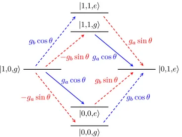
The intermediate states and transitions contributing (in lowest order) to the |1, 0, g〉 ↔ |0, 1, e〉 transition are shown in Fig. 2. Virtual transitions to and from one of the four intermediate states |0, 0, g〉, |0, 0, e〉, |1, 1, g〉, and |1, 1, e〉 connect |1, 0, g〉 and |0, 1, e〉 in two steps. This is the minimum number of steps possible, since the terms in the Hamiltonian in Eq. (1) can only create or annihilate a single photon at a time. From the figure, it is also clear that no path exists between |1, 0, g〉 and |0, 1, e〉 that does not involve longitudinal coupling (dashed red arrows in the figure).
To calculate the effective coupling between the states |1, 0, g〉 and |0, 1, e〉, we truncate the Hamiltonian from Eq. (1) to the six states shown in Fig. 2. Written on matrix form, this truncated Hamiltonian becomes
Figure 2. The four lowest-order processes contributing to a transition between |1, 0, g〉 and |0, 1, e〉. For this illustration, the parameter values ωa = 3ωq and ωb = 2ωq were used to set the positions of the energy levels. The
transitions that do not conserve excitation number are shown as dashed lines, and the excitation-number-conserving transitions are shown as solid lines. Red lines correspond to σˆz (longitudinal) coupling and blue lines
ω θ θ ω θ θ θ θ ω ω θ θ θ θ ω ω θ θ θ θ ω ω ω θ θ ω ω ω = − − − − − + − + − + + ˆH g g g g g g g g g g g g g g g g 2 0 sin cos 0 0 0 2 cos sin 0 0 sin cos 2 0 sin cos cos sin 0 2 cos sin 0 0 sin cos 2 0 0 0 cos sin 0 2 , (3) q a b q a b a a a q b b b b b q a a b a a b q b a a b q
where the states are ordered from left to right as |0, 0, g〉, |0, 0, e〉, |1, 0, g〉, |0, 1, e〉, |1, 1, g〉, and |1, 1, e〉. When the condition ωa ≈ ωb + ωq is satisfied, the four intermediate states |0, 0, g〉, |0, 0, e〉, |1, 1, g〉, and |1, 1, e〉 can be
adia-batically eliminated, i.e., provided that the bare coupling strengths are sufficiently small compared to the energy difference between the intermediate states and the initial and final states, we can assume that the population of the intermediate states will not change significantly, such that the effective dynamics will only involve the initial and final states. This calculation, shown in the Supplementary Information, gives an effective Hamiltonian with a coupling term
= +
ˆHc,eff geff( 1, 0,g 0, 1,e 0, 1,e 1, 0, ),g (4) where the effective coupling between the states |1, 0, g〉 and |0, 1, e〉 has the magnitude
θ ω ω = − g g g sin2 1 1 (5) a b b a eff
on resonance. Compared to the direct resonator-qubit coupling in Eq. (1), geff is weaker by a factor of order g/ω,
which is why we need to at least approach the USC regime to observe the single-photon frequency conversion. We note that the effective coupling is maximised when the longitudinal and transverse coupling terms in Eq. (1) have equal magnitude. Interestingly, Eq. (5) suggests that frequency conversion can be more efficient if ωb ≪ ωa.
However, going too far in this direction violates the assumptions behind the adiabatic approximation, which relies on ga,gb ≪ ωa,ωb.
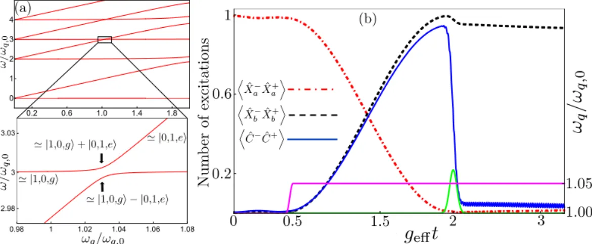
The existence of this effective coupling suggests at least two ways to perform single-photon frequency con-version. The first is to use adiabatic transfer, starting in |1, 0, g〉 (|0, 1, e〉) with the qubit frequency sufficiently far detuned from the resonance ωa = ωb + ωq and then slowly [adiabatically, i.e., slow enough that the probability of
a Landau-Zener transition back to the initial state is small; note that this is a different notion of adiabaticity than that used in the adiabatic elimination used to derive Eq. (4)] changing the qubit frequency until the system ends up in the state |0, 1, e〉 (|1, 0, g〉), following one of the energy levels shown in Fig. 3(a). In this way, a single photon in the first (second) resonator is deterministically down-converted (up-converted) to a single photon of lower (higher) frequency in the second (first) resonator. We note that such adiabatic transfer has been used for robust single-photon generation in circuit QED, tuning the frequency of a transmon qubit to achieve the transition |0, e〉 → |1, g〉91. It has also been suggested as a method to generate multiple photons from a single qubit excitation in the USC regime of the standard quantum Rabi model68.
The second approach, exemplified by a simulation including decoherence in Fig. 3(b), is to initialise the sys-tem in one of the states |1, 0, g〉 or |0, 1, e〉, far from the frequency-conversion resonance such that the effective coupling is negligible, quickly tune the qubit into resonance for the duration of half a Rabi oscillation period (set by the effective coupling to be π/2geff), and then detune the qubit again (or send a pulse to deexcite it) to turn off
the effective interaction. This type of scheme is, for example, commonly used for state transfer between resonators and/or qubits in circuit QED92–96. Letting the resonance last shorter or longer times, any superposition of |1, 0, g〉 or |0, 1, e〉 can be created. The potential for creating superpositions of photons of different frequencies (similar to ref. 27) with such a method will be explored in future work.
Since the relevant timescales for both these approaches are determined by geff, it is important to know in which
parameter range the expression for geff given in Eq. (5) remains a good approximation. In Fig. 4, we show that the
expression is valid up to at least ga = gb = 0.2ωq,0 for the parameters used in Fig. 3.
We note that both protocols for frequency-conversion given here can be used to transfer superposition states. For example, starting in the superposition state a|0, 0, g〉 + b|1, 0, g〉 = (a|0〉 + b|1〉)|0, g〉, where a and b are com-plex numbers satisfying |a|2 + |b|2 = 1, both protocols will convert this state into a|0, 0, g〉 + b|0, 1, e〉 = |0〉(a|0,
g〉 + b|1, e〉). If one wishes to disentangle the qubit from the second resonator mode after the transfer of the super-position, a photon-number-dependent qubit rotation, which can be implemented in the strong-dispersive regime of circuit QED97, is one option. The remarks given here also apply to the multi-photon frequency-conversion processes studied in the next section.
Multi-photon frequency conversion.
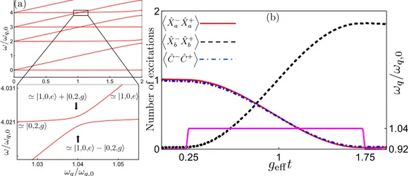
We now turn to multi-photon frequency conversion, where, aided by the qubit, one photon in the first resonator is converted into two photons in the second resonator, or vice versa. We continue to adopt the convention that ωa > ωb. In contrast to the single-photon frequency conversion caseabove, there are now two possibilities for how the qubit state can change during the conversion process. Below, we will study both |1, 0, g〉 ↔ |0, 2, e〉 and |1, 0, e〉 ↔ |0, 2, g〉. Since we wish to use the qubit to control the process, we do not consider the process |1, 0, g〉 ↔ |0, 2, g〉, which to some extent was already included in ref. 80, although that work considered a setup with ωq ≈ ωb and mainly studied the squeezing produced by a strong external drive.
The |1, 0, g
〉 ↔ |0,2,e〉 process.
For the process |1, 0, g〉 ↔ |0, 2, e〉, we first of all note one more difference compared to the single-photon frequency conversion case: it changes the number of excitations from 1 to 3, which means that excitation-number parity is conserved. This makes the longitudinal coupling of Eq. (1) redundant for achieving the conversion, and to simplify our calculations we therefore hereafter work with the standard quantum Rabi Hamiltonian98 extended to two resonators,Figure 3. Two frequency conversion methods. (a) The figure shows the energy levels of our system plotted as a function of the qubit frequency ωq, using the parameters ga = gb = 0.15ωq,0, θ = π/6, ωa = 3ωq,0, and ωb = 2ωq,0,
where ωq,0 is a reference point for the qubit frequency, set such that ωa = ωb + ωq,0. In the zoom-in, close to the
resonance ωa = ωb + ωq, we see the anticrossing between |1, 0, g〉 and |0, 1, e〉 with splitting 2geff. Up- or
down-conversion of single photons can be achieved by adiabatically tuning ωq to follow one of the energy levels in the
figure from |1, 0, g〉 to |0, 1, e〉, or vice versa. (b) A rapid frequency conversion can be achieved by starting in |1, 0, g〉, far from the resonance ωa = ωb + ωq, tuning the qubit frequency (pink solid curve) into resonance for half a
Rabi period (π/2geff) and then sending a pulse (green solid curve) to deexcite the qubit. The pink solid curve is
given by ωq( )t =ωq i, +δωq{sin [ (2A t−ti)] (Θ −t ti)+sin [ (2A t−tf)] (Θ −t tf)}, a smoothed step function, where ωq,i is the initial qubit frequency, δωq is the change of the qubit frequency, Θ is the Heaviside step
function, ti is the time when the qubit frequency starts to change, tf = ti + π/(2A), and A is a frequency setting
the smoothness. The figure shows the number of excitations in the two resonators (red dashed-dotted curve for a, black dashed curve for b) and the qubit (blue solid curve) during the process, including decoherence in the form of relaxation from the resonators and the qubit. The parameters used for the decoherence are
κa = κb = γ = 4 × 10⁻⁵ωq,0.
Figure 4. Comparison of analytical (red curve) and numerical (black dots) results for the effective coupling between the states |1, 0, g〉 and |0, 1, e〉. The graph shows the minimum energy splitting 2geff/ωq,0 as a function of
ω ω ωσ σ = + + + + + + . ˆ ˆ ˆ† ˆ ˆ† ˆ ˆ ˆ† ˆ ˆ ˆ† H a a b b g a a g b b 2 [ ( ) ( )] (6) a b q z a b x R
Placing the system close to the resonance ωa = 2ωb + ωq, virtual transitions involving the intermediate states
|0, 0, e〉, |0, 1, g〉, |1, 1, e〉, and |1, 2, g〉 (to lowest order), contribute to the process |1, 0, g〉 ↔ |0, 2, e〉, as shown in Fig. 5. The most direct path between |1, 0, g〉 and |0, 2, e〉 involves three steps, since only one photon can be created or annihilated in each step. We note that all the paths include at least one transition that is due to terms in the Hamiltonian that do not conserve excitation number (dashed arrows in the figure).
Retaining only the states shown in Fig. 5, we can write the quantum Rabi Hamiltonian from Eq. (6) on matrix form as ω ω ω ω ω ω ω ω ω ω ω ω ω = − − + + + + − ˆH g g g g g g g g g g g g g g 2 0 0 0 2 0 2 0 0 2 0 0 0 2 0 2 2 0 0 0 2 2 0 0 0 2 2 2 , (7) q b a b b q b a a a q b b b q a a b a b q b a b a b q R
where the states are ordered as |0, 0, e〉, |0, 1, g〉, |1, 0, g〉, |0, 2, e〉, |1, 1, e〉, and |1, 2, g〉. Just like before, we can adiabatically eliminate the intermediate states when the condition ωa ≈ 2ωb + ωq is satisfied. The result of this
calculation, the details of which are given in the Supplementary Information, is an effective coupling between the states |1, 0, g〉 and |0, 2, e〉 with magnitude
ω ω ω ω ω ω ω ω ω = − − − + − + g g g g g 2 [2 ( 2 ) ] 2 ( ) (5 3 ) (8) b a b b a b b b a eff 3 2 2 2 2 4
on resonance. Here, we have set ga = gb ≡ g to simplify the expression slightly. We note that, to leading order, the
coupling scales like g3/ω2; indeed, the leading-order term is
ω ω ω ω ω = − − . g 2 (g 2 ) ( ) (9) a b b a b eff 3 2
This is a factor g/ω weaker than for the single-photon frequency conversion, and reflects the fact that an addi-tional intermediate transition is required for the two-photon conversion. We also note that the coupling becomes Figure 5. The lowest-order processes contributing to a transition between |1, 0, g〉 and |0, 2, e〉 in the quantum Rabi model. The transitions that do not conserve excitation number are shown as dashed blue lines and the excitation-number-conserving transitions are shown as solid blue lines. The label of each line is the term in Eq. (6) that gives rise to that transition. The parameters ωa = 5ωq and ωb = 2ωq were used to set the positions of the
small in the limit of small ωq, i.e., when 2ωb → ωa. The coupling would become large if ωa → ωb, but this is
impos-sible since ωa = 2ωb + ωq in this scheme.
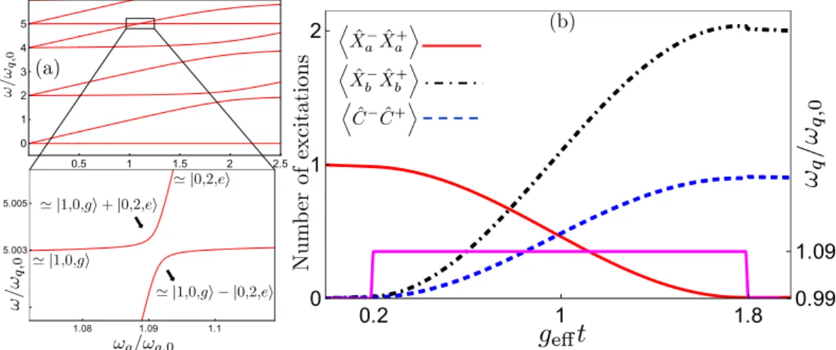
The two-photon frequency conversion can be performed either by adiabatic transfer or by tuning the qubit into resonance for half a Rabi oscillation period, as explained in the section on single-photon frequency conver-sion. In the first approach, one adiabatically tunes the qubit energy to follow one of the energy levels shown in Fig. 6(a). A simulation of the second approach, including decoherence, is shown in Fig. 6(b). The timescale for these processes is set by the effective coupling. In Fig. 7, we show that the expression for the effective coupling given in Eq. (8) remains a good approximation up to at least g = 0.3ωq,0 for the parameters used in Fig. 6.
The |1, 0, e
〉 ↔ |0, 2, g〉 process.
For the process |1, 0, e〉 ↔ |0, 2, g〉, we show in Fig. 8 the virtual transi-tions from the quantum Rabi Hamiltonian that contribute to lowest order. We note that this process conserves the excitation number, which means that there is a path between the states that can be realised using only terms from Figure 6. Two-photon frequency conversion via transitions between |1, 0, g〉 and |0, 2, e〉. (a) The energy levels of our system, given in Eq. (6), plotted as a function of the qubit frequency ωq, using the parametersga = gb = 0.2ωq,0, ωa = 5ωq,0, and ωb = 2ωq,0, where the reference point ωq,0 is set such that ωa = 2ωb + ωq,0. In
the zoom-in, close to the resonance ωa = 2ωb + ωq, we see the anticrossing between |1, 0, g〉 and |0, 2, e〉 with
the splitting 2geff given by Eq. (8). Up-conversion of a photon pair into a single photon, or down-conversion
of a single photon into a photon pair, can be achieved by adiabatically tuning ωq to follow one of the energy
levels in the figure from |0, 2, e〉 to |1, 0, g〉, or vice versa. (b) A rapid frequency conversion can be achieved by starting in |1, 0, g〉 or |0, 2, e〉, far from the resonance ωa = 2ωb + ωq, tuning the qubit frequency (pink solid
curve, a smoothed step function as explained in Fig. 3) into resonance for half a Rabi period (π/2geff) and
then tuning it out of resonance again. The figure shows the number of excitations in the two resonators (red solid curve for a, black dashed-dotted curve for b) and the qubit (blue dashed curve) during such a process, including decoherence in the form of relaxation from the resonators and the qubit. The parameters used for the decoherence are κa = κb = γ = 2 × 10⁻⁵ωq,0.
Figure 7. Comparison of analytical (red curve) and numerical (black dots) results for the effective coupling between the states |1, 0, g〉 and |0, 2, e〉. The graph shows the minimum energy splitting 2geff/ωq,0 as a function of
the Jaynes–Cummings (JC) Hamiltonian99 (solid arrows in the figure). Below, we analyse the effective coupling both for the full quantum Rabi Hamiltonian and for the JC Hamiltonian. Usually, the JC Hamiltonian is obtained by performing the RWA on the quantum Rabi Hamiltonian when g ≪ ωa/b/q, in which case the low coupling
strength would make it very challenging to observe the frequency conversion process. However, we note that a circuit QED setup has been proposed where the pure JC Hamiltonian with ultrastrong coupling can be realised100.
Quantum Rabi Hamiltonian.
Retaining only the states shown in Fig. 8, we can write the quantum Rabi Hamiltonian from Eq. (6) on matrix form asω ω ω ω ω ω ω ω ω ω ω ω ω = − + + − + − + + ˆH g g g g g g g g g g g g g g 2 0 0 0 2 0 2 0 0 2 0 0 0 2 0 2 2 0 0 0 2 2 0 0 0 2 2 2 , (10) q b a b b q b a a a q b b b q a a b a b q b a b a b q R
where the states are ordered as |0, 0, g〉, |0, 1, e〉, |1, 0, e〉, |0, 2, g〉, |1, 1, g〉, and |1, 2, e〉. As in previous calculations, we can perform adiabatic elimination close to the resonance, which in this case is ωa + ωq ≈ 2ωb. The details of
the elimination are given in the Supplementary Information. The result is an effective coupling between the states |1, 0, e〉 and |0, 2, g〉 with magnitude
ω ω ω ω ω ω ω ω ω = − − − + − + g g g g g 2 [2 ( 2 ) ] 2 ( ) (5 3 ) (11) b a b b a b b b a eff 3 2 2 2 2 4
on resonance. We have set ga = gb ≡ g to simplify the expression slightly. Note that this expression for the coupling
is actually exactly the same as the one for the process |1, 0, g〉 ↔ |0, 2, e〉 given in Eq. (8). Even though the two processes use different intermediate states, the truncated Hamiltonians in Eqs (7) and (10) only differ in the sign of ωq. Since ωq is replaced on resonance by (ωa − 2ωb) in the first case and by (2ωb − ωa) in the second case, the
formula for the effective coupling ends up being the same in both cases. The two cases still differ, however. For example, while the limit ωa → ωb, which enhances the coupling, could not occur for the process |1, 0, g〉 ↔ |0, 2,
e〉, it is possible for |1, 0, e〉 ↔ |0, 2, g〉. However, in this limit the approximations behind the adiabatic elimination break down, since the states |1, 1, g〉 and |0, 1, e〉 would also be on resonance and become populated.
The two-photon frequency conversion can again be performed either by adiabatic transfer or by tuning the qubit into resonance for half a Rabi oscillation period, as explained in the section on single-photon frequency Figure 8. The lowest-order processes contributing to a transition between |1, 0, e〉 and |0, 2, g〉 in the quantum Rabi model. The transitions that do not conserve excitation number are shown as dashed blue lines and the excitation-number-conserving transitions are shown as solid blue lines. The label of each line is the term in Eq. (6) that gives rise to that transition. The parameters ωa = 3ωq and ωb = 2ωq were used to set the positions of the
conversion. The energy levels to follow in the first approach are plotted in Fig. 9(a) and a simulation of the second approach, including decoherence, is shown in Fig. 9(b).
Jaynes–Cummings Hamiltonian.
For completeness, we calculate the effective coupling using only the JC Hamiltonian for two resonators and one qubit, i.e., we eliminate the non-excitation-conserving terms in the quantum Rabi Hamiltonian of Eq. (6), givingω ω ω σ σ σ σ σ = + + + ++ − + ++ − . ˆ ˆ ˆ† ˆ ˆ† ˆ ˆ ˆ ˆ ˆ†
(
ˆ ˆ ˆ ˆ†)
H a a b b g a a g b b 2 ( ) (12) a b q z a b JCRetaining only the states connected by solid arrows in Fig. 8, we can write the Hamiltonian from Eq. (12) on matrix form as ω ω ω ω ω ω ω ω ω = + + − + − ˆH g g g g g g 2 0 2 0 2 0 2 0 2 2 0 0 2 , (13) b q b a a q b b b q a b a b q JC
where the states are ordered as |0, 1, e〉, |1, 0, e〉, |0, 2, g〉, and |1, 1, g〉. Again, we perform adiabatic elimination close to the resonance ωa + ωq ≈ 2ωb. The details of the elimination are given in the Supplementary Information.
The result is an effective coupling between the states |1, 0, e〉 and |0, 2, g〉 with magnitude
ω ω = − + − g g g g 2 ( a b ) (14) a a b eff 2 2 2
on resonance. Just as for the other two-photon frequency-conversion processes, the coupling scales like g3/ω2 to
leading order. In fact, Eq. (14) is a good approximation to Eq. (11), since the path given by the JC terms (solid lines) in Fig. 8 is far less detuned in energy from the initial and final states than all the other paths and thus gives the largest contribution to the result in Eq. (11). The remarks on the limit ωa → ωb given after Eq. (11) apply here
as well. The schemes for implementing the frequency conversion are already given in Fig. 9.
Figure 9. Two-photon frequency conversion via transitions between |1, 0, e〉 and |0, 2, g〉. (a) The energy levels of our system, given in Eq. (6), plotted as a function of the qubit frequency ωq, using the parameters
ga = gb = 0.125ωq,0, ωa = 3ωq,0, and ωb = 2ωq,0, where the reference point ωq,0 is set such that ωa + ωq,0 = 2ωb. In
the zoom-in, close to the resonance ωa + ωq = 2ωb, we see the anticrossing between |1, 0, e〉 and |0, 2, g〉 with
the splitting 2geff given by Eq. (11). Up-conversion of a photon pair into a single photon, or down-conversion
of a single photon into a photon pair, can be achieved by adiabatically tuning ωq to follow one of the energy
levels in the figure from |0, 2, g〉 to |1, 0, e〉, or vice versa. (b) A rapid frequency conversion can be achieved by starting in |1, 0, e〉 or |0, 2, g〉, far from the resonance ωa + ωq = 2ωb, tuning the qubit frequency (pink solid
curve, a smoothed step function as explained in Fig. 3) into resonance for half a Rabi period (π/2geff) and
then tuning it out of resonance again. The figure shows the number of excitations in the two resonators (red solid curve for a, black dashed-dotted curve for b) and the qubit (blue dashed curve) during such a process, including decoherence in the form of relaxation from the resonators and the qubit. The parameters used for the decoherence are κa = κb = γ = 4 × 10⁻⁵ωq,0.
In Fig. 10, we compare the results from Eqs (11) and (14) with a full numerical calculation using the quantum Rabi Hamiltonian. The contribution from the JC part dominates the coupling up until around ga = gb = g = 0.03ωq,0
and gives a good approximation until then. For higher values of the coupling, using the approximation from the quantum Rabi Hamiltonian instead works fine up until around ga = gb = g = 0.15ωq,0. It is interesting to note that
a pure JC Hamiltonian in the USC regime would give higher effective coupling for this frequency-conversion process than the quantum Rabi Hamiltonian.
Discussion
We have shown how a system consisting of two resonators ultrastrongly coupled to a qubit can be used to realise a variety of frequency-conversion processes. In particular, we have shown how to convert a single photon into another photon of either higher or lower frequency, as well as how to convert a single photon into a photon pair and vice versa. All these processes are deterministic, can be implemented within a single setup, and do not require any external drives. The conversion is controlled by tuning the frequency of the qubit to and from values that make the desired transitions resonant.
Given the recent advances in USC circuit QED, we believe that our proposal can be implemented in such a setup. Indeed, two resonators have already been ultrastrongly coupled to a superconducting flux qubit49. Also, our proposal does not require very high coupling strengths. We only need that g2/ω is appreciable (larger than the
relevant decoherence rates) to realise single-photon frequency conversion; multi-photon frequency conversion can be demonstrated if g3/ω2 is large enough.
A straightforward extension of the current work is to extend the calculations to processes with more pho-tons in the second resonator or to add more resonators to the setup. Some of these possibilities are discussed in ref. 71, where we explore analogies of nonlinear optics in USC systems, including the fact that the pro-cesses in the current work can be considered analogies of Raman and hyper-Raman scattering if the qubit is thought of as playing the role of a phonon. More general three-wave mixing, such as |1, 0, 0, e〉 ↔ |0, 1, 1, g〉, or third-harmonic and -subharmonic generation such as |1, 0, e〉 ↔ |0, 3, g〉, are examples of schemes that can be considered, but it must be kept in mind that higher-order processes with more photons involved will have lower effective coupling strengths. Another direction for future work is to investigate how the precise qubit control of the frequency-conversion processes discussed here can be used to prepare photon bundles101 or interesting quantum superposition states with photons of different frequencies, a topic currently being explored in several frequency ranges26, 27, 102.
References
1. Kumar, P. Quantum frequency conversion. Opt. Lett. 15, 1476 (1990).
2. Huang, J. & Kumar, P. Observation of quantum frequency conversion. Phys. Rev. Lett. 68, 2153 (1992). 3. O’Brien, J. L., Furusawa, A. & Vučković, J. Photonic quantum technologies. Nat. Photonics 3, 687 (2009).
4. Buluta, I., Ashhab, S. & Nori, F. Natural and artificial atoms for quantum computation. Reports Prog. Phys. 74, 104401 (2011). 5. Kimble, H. J. The quantum internet. Nature 453, 1023 (2008).
6. Albota, M. A. & Wong, F. N. C. Efficient single-photon counting at 155 μm by means of frequency upconversion. Opt. Lett. 29, 1449 (2004).
7. Tanzilli, S. et al. A photonic quantum information interface. Nature 437, 116 (2005).
8. Ou, Z. Y. Efficient conversion between photons and between photon and atom by stimulated emission. Phys. Rev. A 78, 023819 (2008).
9. Ding, Y. & Ou, Z. Y. Frequency downconversion for a quantum network. Opt. Lett. 35, 2591 (2010). 10. Takesue, H. Single-photon frequency down-conversion experiment. Phys. Rev. A 82, 013833 (2010).
11. Guo, X., Zou, C.-L., Jung, H. & Tang, H. X. On-Chip Strong Coupling and Efficient Frequency Conversion between Telecom and Visible Optical Modes. Phys. Rev. Lett. 117, 123902 (2016).
12. You, J. Q. & Nori, F. Atomic physics and quantum optics using superconducting circuits. Nature 474, 589 (2011).
13. Devoret, M. H. & Schoelkopf, R. J. Superconducting Circuits for Quantum Information: An Outlook. Science 339, 1169 (2013).
Figure 10. Comparison of analytical (JC Hamiltonian [dashed blue curve] and quantum Rabi Hamiltonian [solid red curve]) and numerical (black dots) results for the effective coupling between the states |1, 0, e〉 and |0, 2, g〉. The graph shows the minimum energy splitting 2geff/ωq,0 as a function of g/ωq,0, using the same parameters as in Fig. 9.
Rev. A 82, 052509 (2010).
26. Chirolli, L., Burkard, G., Kumar, S. & DiVincenzo, D. P. Superconducting Resonators as Beam Splitters for Linear-Optics Quantum Computation. Phys. Rev. Lett. 104, 230502 (2010).
27. Zakka-Bajjani, E. et al. Quantum superposition of a single microwave photon in two different ‘colour’ states. Nat. Phys. 7, 599 (2011).
28. Abdo, B. et al. Full Coherent Frequency Conversion between Two Propagating Microwave Modes. Phys. Rev. Lett. 110, 173902 (2013).
29. Kamal, A., Roy, A., Clarke, J. & Devoret, M. H. Asymmetric Frequency Conversion in Nonlinear Systems Driven by a Biharmonic Pump. Phys. Rev. Lett. 113, 247003 (2014).
30. Marquardt, F. Efficient on-chip source of microwave photon pairs in superconducting circuit QED. Phys. Rev. B 76, 205416 (2007). 31. Koshino, K. Down-conversion of a single photon with unit efficiency. Phys. Rev. A 79, 013804 (2009).
32. Sánchez-Burillo, E., Martín-Moreno, L., García-Ripoll, J. J. & Zueco, D. Full two-photon down-conversion of a single photon. Phys.
Rev. A 94, 053814 (2016).
33. Inomata, K. et al. Microwave Down-Conversion with an Impedance-Matched Λ System in Driven Circuit QED. Phys. Rev. Lett.
113, 063604 (2014).
34. Deppe, F. et al. Two-photon probe of the Jaynes–Cummings model and controlled symmetry breaking in circuit QED. Nat. Phys.
4, 686 (2008).
35. Liu, Y.-X., You, J. Q., Wei, L. F., Sun, C. P. & Nori, F. Optical Selection Rules and Phase-Dependent Adiabatic State Control in a Superconducting Quantum Circuit. Phys. Rev. Lett. 95, 087001 (2005).
36. Liu, Y.-X. et al. Controllable microwave three-wave mixing via a single three-level superconducting quantum circuit. Sci. Rep. 4, 7289 (2014).
37. Lecocq, F., Clark, J. B., Simmonds, R. W., Aumentado, J. & Teufel, J. D. Mechanically Mediated Microwave Frequency Conversion in the Quantum Regime. Phys. Rev. Lett. 116, 043601 (2016).
38. Günter, G. et al. Sub-cycle switch-on of ultrastrong light–matter interaction. Nature 458, 178 (2009).
39. Forn-Díaz, P. et al. Observation of the Bloch-Siegert Shift in a Qubit-Oscillator System in the Ultrastrong Coupling Regime. Phys.
Rev. Lett. 105, 237001 (2010).
40. Niemczyk, T. et al. Circuit quantum electrodynamics in the ultrastrong-coupling regime. Nat. Phys. 6, 772 (2010). 41. Todorov, Y. et al. Ultrastrong Light-Matter Coupling Regime with Polariton Dots. Phys. Rev. Lett. 105, 196402 (2010).
42. Schwartz, T., Hutchison, J. A., Genet, C. & Ebbesen, T. W. Reversible Switching of Ultrastrong Light-Molecule Coupling. Phys. Rev.
Lett. 106, 196405 (2011).
43. Scalari, G. et al. Ultrastrong Coupling of the Cyclotron Transition of a 2D Electron Gas to a THz Metamaterial. Science 335, 1323 (2012).
44. Geiser, M. et al. Ultrastrong Coupling Regime and Plasmon Polaritons in Parabolic Semiconductor Quantum Wells. Phys. Rev. Lett.
108, 106402 (2012).
45. Kéna-Cohen, S., Maier, S. A. & Bradley, D. D. C. Ultrastrongly Coupled Exciton-Polaritons in Metal-Clad Organic Semiconductor Microcavities. Adv. Opt. Mater. 1, 827 (2013).
46. Gambino, S. et al. Exploring Light–Matter Interaction Phenomena under Ultrastrong Coupling Regime. ACS Photonics 1, 1042 (2014).
47. Maissen, C. et al. Ultrastrong coupling in the near field of complementary split-ring resonators. Phys. Rev. B 90, 205309 (2014). 48. Goryachev, M. et al. High-Cooperativity Cavity QED with Magnons at Microwave Frequencies. Phys. Rev. Appl. 2, 054002 (2014). 49. Baust, A. et al. Ultrastrong coupling in two-resonator circuit QED. Phys. Rev. B 93, 214501 (2016).
50. Forn-Díaz, P. et al. Ultrastrong coupling of a single artificial atom to an electromagnetic continuum in the nonperturbative regime.
Nat. Phys. 13, 39 (2017).
51. Yoshihara, F. et al. Superconducting qubit-oscillator circuit beyond the ultrastrong-coupling regime. Nat. Phys. 13, 44 (2017). 52. Chen, Z. et al. Multi-photon sideband transitions in an ultrastrongly-coupled circuit quantum electrodynamics system.
arXiv:1602.01584 (2016).
53. George, J. et al. Multiple Rabi Splittings under Ultrastrong Vibrational Coupling. Phys. Rev. Lett. 117, 153601 (2016).
54. Langford, N. K. et al. Experimentally simulating the dynamics of quantum light and matter at ultrastrong coupling.
arXiv:1610.10065 (2016).
55. Braumüller, J. et al. Analog quantum simulation of the Rabi model in the ultra-strong coupling regime. arXiv:1611.08404 (2016). 56. Yoshihara, F. et al. Characteristic spectra of circuit quantum electrodynamics systems from the ultrastrong to the deep strong
coupling regime. Phys. Rev. A 95, 053824 (2017).
57. De Liberato, S., Ciuti, C. & Carusotto, I. Quantum Vacuum Radiation Spectra from a Semiconductor Microcavity with a Time-Modulated Vacuum Rabi Frequency. Phys. Rev. Lett. 98, 103602 (2007).
58. Ashhab, S. & Nori, F. Qubit-oscillator systems in the ultrastrong-coupling regime and their potential for preparing nonclassical states. Phys. Rev. A 81, 042311 (2010).
59. Cao, X., You, J. Q., Zheng, H., Kofman, A. G. & Nori, F. Dynamics and quantum Zeno effect for a qubit in either a low- or high-frequency bath beyond the rotating-wave approximation. Phys. Rev. A 82, 022119 (2010).
60. Cao, X., You, J. Q., Zheng, H. & Nori, F. A qubit strongly coupled to a resonant cavity: asymmetry of the spontaneous emission spectrum beyond the rotating wave approximation. New J. Phys. 13, 073002 (2011).
61. Stassi, R., Ridolfo, A., Di Stefano, O., Hartmann, M. J. & Savasta, S. Spontaneous Conversion from Virtual to Real Photons in the Ultrastrong-Coupling Regime. Phys. Rev. Lett. 110, 243601 (2013).
62. Sanchez-Burillo, E., Zueco, D., Garcia-Ripoll, J. J. & Martin-Moreno, L. Scattering in the Ultrastrong Regime: Nonlinear Optics with One Photon. Phys. Rev. Lett. 113, 263604 (2014).
63. De Liberato, S. Light-Matter Decoupling in the Deep Strong Coupling Regime: The Breakdown of the Purcell Effect. Phys. Rev. Lett.
112, 016401 (2014).
64. Lolli, J., Baksic, A., Nagy, D., Manucharyan, V. E. & Ciuti, C. Ancillary Qubit Spectroscopy of Vacua in Cavity and Circuit Quantum Electrodynamics. Phys. Rev. Lett. 114, 183601 (2015).
65. Di Stefano, O. et al. Feynman-diagrams approach to the quantum Rabi model for ultrastrong cavity QED: stimulated emission and reabsorption of virtual particles dressing a physical excitation. New J. Phys19, 053010 (2016).
66. Cirio, M., De Liberato, S., Lambert, N. & Nori, F. Ground State Electroluminescence. Phys. Rev. Lett. 116, 113601 (2016). 67. Zhu, G., Ferguson, D. G., Manucharyan, V. E. & Koch, J. Circuit QED with fluxonium qubits: Theory of the dispersive regime. Phys.
Rev. B 87, 024510 (2013).
68. Ma, K. K. W. & Law, C. K. Three-photon resonance and adiabatic passage in the large-detuning Rabi model. Phys. Rev. A 92, 023842 (2015).
69. Garziano, L. et al. Multiphoton quantum Rabi oscillations in ultrastrong cavity QED. Phys. Rev. A 92, 063830 (2015). 70. Garziano, L. et al. One Photon Can Simultaneously Excite Two or More Atoms. Phys. Rev. Lett. 117, 043601 (2016).
71. Kockum, A. F., Miranowicz, A., Macrì, V., Savasta, S. & Nori, F. Deterministic quantum nonlinear optics with single atoms and virtual photons. Phys. Rev. A arXiv:1701.05038 (2017).
72. Buluta, I. & Nori, F. Quantum Simulators. Science 326, 108 (2009).
73. Georgescu, I. M., Ashhab, S. & Nori, F. Quantum simulation. Rev. Mod. Phys. 86, 153 (2014). 74. Braak, D. Integrability of the Rabi Model. Phys. Rev. Lett. 107, 100401 (2011).
75. Braak, D. Solution of the Dicke model for N=3. J. Phys. B At. Mol. Opt. Phys. 46, 224007 (2013).
76. Peng, J., Ren, Z., Guo, G., Ju, G. & Guo, X. Exact solutions of the generalized two-photon and two-qubit Rabi models. Eur. Phys. J.
D 67, 162 (2013).
77. Chilingaryan, S. A. & Rodríguez-Lara, B. M. Exceptional solutions in two-mode quantum Rabi models. J. Phys. B At. Mol. Opt.
Phys. 48, 245501 (2015).
78. Duan, L., He, S., Braak, D. & Chen, Q.-H. Solution of the two-mode quantum Rabi model using extended squeezed states.
Europhys. Lett. 112, 34003 (2015).
79. Alderete, C. H. & Rodríguez-Lara, B. M. Cross-cavity quantum Rabi model. J. Phys. A Math. Theor. 49, 414001 (2016).
80. Moon, K. & Girvin, S. M. Theory of Microwave Parametric Down-Conversion and Squeezing Using Circuit QED. Phys. Rev. Lett.
95, 140504 (2005).
81. Mariantoni, M. et al. Two-resonator circuit quantum electrodynamics: A superconducting quantum switch. Phys. Rev. B 78, 104508 (2008).
82. Prado, F. O., de Almeida, N. G., Moussa, M. H. Y. & Villas-Bôas, C. J. Bilinear and quadratic Hamiltonians in two-mode cavity quantum electrodynamics. Phys. Rev. A 73, 043803 (2006).
83. You, J. Q., Hu, X., Ashhab, S. & Nori, F. Low-decoherence flux qubit. Phys. Rev. B 75, 140515 (2007).
84. Kim, Z. et al. Decoupling a Cooper-Pair Box to Enhance the Lifetime to 0.2 ms. Phys. Rev. Lett. 106, 120501 (2011). 85. Beaudoin, F., Gambetta, J. M. & Blais, A. Dissipation and ultrastrong coupling in circuit QED. Phys. Rev. A 84, 043832 (2011). 86. Ridolfo, A., Leib, M., Savasta, S. & Hartmann, M. J. Photon Blockade in the Ultrastrong Coupling Regime. Phys. Rev. Lett. 109,
193602 (2012).
87. Megrant, A. et al. Planar superconducting resonators with internal quality factors above one million. Appl. Phys. Lett. 100, 113510 (2012).
88. Stern, M. et al. Flux Qubits with Long Coherence Times for Hybrid Quantum Circuits. Phys. Rev. Lett. 113, 123601 (2014). 89. Orgiazzi, J.-L. et al. Flux qubits in a planar circuit quantum electrodynamics architecture: Quantum control and decoherence. Phys.
Rev. B 93, 104518 (2016).
90. Yan, F. et al. The flux qubit revisited to enhance coherence and reproducibility. Nat. Commun. 7, 12964 (2016).
91. Johnson, B. R. et al. Quantum non-demolition detection of single microwave photons in a circuit. Nat. Phys. 6, 663 (2010). 92. Sillanpää, M. A., Park, J. I. & Simmonds, R. W. Coherent quantum state storage and transfer between two phase qubits via a
resonant cavity. Nature 449, 438 (2007).
93. Hofheinz, M. et al. Generation of Fock states in a superconducting quantum circuit. Nature 454, 310 (2008). 94. Hofheinz, M. et al. Synthesizing arbitrary quantum states in a superconducting resonator. Nature 459, 546 (2009).
95. Wang, H. et al. Deterministic Entanglement of Photons in Two Superconducting Microwave Resonators. Phys. Rev. Lett. 106, 060401 (2011).
96. Mariantoni, M. et al. Photon shell game in three-resonator circuit quantum electrodynamics. Nat. Phys. 7, 287 (2011). 97. Schuster, D. I. et al. Resolving photon number states in a superconducting circuit. Nature 445, 515 (2007).
98. Rabi, I. I. Space Quantization in a Gyrating Magnetic Field. Phys. Rev. 51, 652 (1937).
99. Jaynes, E. T. & Cummings, F. W. Comparison of quantum and semiclassical radiation theories with application to the beam maser.
Proc. IEEE 51, 89 (1963).
100. Baksic, A. & Ciuti, C. Controlling Discrete and Continuous Symmetries in “Superradiant” Phase Transitions with Circuit QED Systems. Phys. Rev. Lett. 112, 173601 (2014).
101. Sánchez Muñoz, C. et al. Emitters of N-photon bundles. Nat. Photonics 8, 550 (2014).
102. Clemmen, S., Farsi, A., Ramelow, S. & Gaeta, A. L. Ramsey Interference with Single Photons. Phys. Rev. Lett. 117, 223601 (2016).
Acknowledgements
We acknowledge useful discussions with Roberto Stassi and Adam Miranowicz. This work is partially supported by the RIKEN iTHES Project, the MURI Center for Dynamic Magneto-Optics via the AFOSR award number FA9550-14-1-0040, the Japan Society for the Promotion of Science (KAKENHI), the IMPACT program of JST, JSPS-RFBR grant No 17-52-50023, CREST grant No. JPMJCR1676, and the Sir John Templeton Foundation. A.F.K. acknowledges support from a JSPS Postdoctoral Fellowship for Overseas Researchers.
Author Contributions
A.F.K. developed the idea and performed the analytical calculations. V.M. and L.G. performed the numerical simulations. S.S. and F.N. supervised the project. A.F.K. wrote the paper with input from all authors.
![Figure 10. Comparison of analytical (JC Hamiltonian [dashed blue curve] and quantum Rabi Hamiltonian [solid red curve]) and numerical (black dots) results for the effective coupling between the states |1, 0, e〉 and |0, 2, g〉](https://thumb-eu.123doks.com/thumbv2/123dokorg/4612816.40190/10.892.241.593.71.320/comparison-analytical-hamiltonian-hamiltonian-numerical-results-effective-coupling.webp)
