Chord sequences : evaluating the effect of complexity on preference

(1)

POLITECNICO DIMILANO

DIPARTIMENTO DI ELETTRONICA EINFORMAZIONE

CORSO DI LAUREAMAGISTRALE ININGEGNERIAINFORMATICA

C

HORD

S

EQUENCES

:

EVALUATING THE EFFECT OF

COMPLEXITY ON PREFERENCE

Master graduation thesis by :

Francesco Foscarin

Supervisor:

Prof. Prof. Augusto Sarti

Assistant supervisor:

Prof. Dr. Bruno Di Giorgi

(2)

(3)

Abstract

W

HATis the level of complexity that we like most when we listen to music? This is the fundamental question that motivates this work. It is not easy to give an answer; yet, music recommendation systems would benefit enormously from an algorithm that could use a currently unused musical property, such as com-plexity, to predict which music the users prefer. In order to answer this question, we exploit the subdivision of music in multiple aspects, such as chords, rhythm, melody, orchestration, etc. and we proceed by using the "divide et conquer" strategy, addressing specifically the task of understanding the relation between preference and complexity of chord sequences.

We know from previous research that some properties, e.g. complexity, tend to increase the amount of activity in the listener’s brain (a.k.a. arousal potential) and we know that this parameter influences the listener’s preference for a certain piece of music. In particular, there is an optimal arousal potential that causes maximum liking, while a too low as well as a too high arousal potential results in a decrease of liking.

We hypothesize that the the level of the optimal arousal potential depends on the mu-sic expertise of a person. Therefore, we design a listening test in order to prove the existence of a relation between these two values. As a measure of complexity, we use a set of state of the art models of harmonic complexity, based on chord sequence probability. Our results, analyzed using robust regression techniques, show a positive correlation between the musical expertise of the subjects who participated in the test and the complexity of the chord sequences that they chose as the one they prefer.

(4)

(5)

Summary

Q

UAL è il livello di complessità che preferiamo durante l’ascolto di musica?

Questa è la domanda fondamentale che motiva il nostro lavoro. Nonostante sia complicato trovare una risposta adeguata, i sistemi di raccomandazione in am-bito musicale trarrebbero grandi benefici da un algoritmo in grado di usare una propri-età musicale attualmente inutilizzata (la complessità) per suggerire la musica preferita dagli utenti. Per rispondere a questa domanda, sfruttiamo la suddivisione della mu-sica in molteplici aspetti, come gli accordi, il ritmo, la melodia, l’orchestrazione, ecc... e utilizziano la strategia "divide et impera", considerando solamente la relazione tra preferenza e complessità delle sequenze di accordi.

Sappiamo da precedenti ricerche che alcune proprietà, tra cui la complessità, tendono ad aumentare la quantità di attività cerebrale dell’ascoltatore (il cosidetto "arousal po-tential"). Inoltre sappiamo che questo parametro influenza la preferenza dell’ascoltatore. In particolare è possibile individuare un "arousal potential" ottimale che produce il mas-simo gradimento, mentre livelli troppo alti e troppo bassi di questo fattore determinano un minor apprezzamento del brano.

In questo lavoro ipotizziamo che il livello ottimale di "arousal potential" dipendenda dall’esperienza musicale di ogni individuo. Pertanto, progettiamo un test di ascolto che punta a verificare l’esistenza di una relazione tra questi due valori. Come misura della complessità usiamo un insieme di modelli di complessità allo stato dell’arte, che si basa sulla probabilità delle sequenze di accordi. Analizzando i nostri risultati attraverso tecniche di regressione robusta, proviamo l’esistenza di una correlazione positiva tra l’esperienza musicale del soggetto e la complessità delle sequenze di accordi da lui preferite.

(6)

(7)

List of Figures

1.1 Complete order (left), chaos (center) and complete disorder (right)

[Fig-ure taken from [18]]. . . 2

1.2 Inverted U-shape curve of complexity and preference . . . 4

2.1 Most used scale in Western music . . . 9

2.2 Melodic Interval vs. Harmonic Interval . . . 9

2.3 The common names used for the intervals between the starting note of a major scale and the other notes. . . 10

2.4 The harmonic inversion of a major sixth. This operation can change the name of the interval. . . 11

2.5 The three possible inversions of a triads. It is possible to still uniquely identify the note generated by the superposition if third, using the names "root", "third" adn "fifth". . . 11

2.6 Harmonization of major and minor (harmonic) scale. . . 12

2.7 A dominant seventh chord built on the V degree of the C major scale. . 12

2.8 The two marginal probabilities of a joint probability distribution of two variables. . . 15

2.9 A graphical model representing the probability distribution defined in the equation 2.16. The node represents the random variables and the arrows represent a variable conditioning another variable . . . 18

2.10 Two different graphical models. The shadowed node in (b) represents an observed node. . . 19

2.11 A probabilistic graphical model for chord progressions. Numbers in level 1 and 2 nodes indicate a particular form of parameter sharing [Fig-ure taken from [50]] . . . 25

2.12 The result of the probe tone experiment for C major and A minor keys. Listeners rated how well the specific tone sounds conclusive . . . 26

3.1 A first order Markov Model. Each variable xiis conditioned only on the value on the previous variable xi−1. . . 28

(10)

3.2 A second order Markov Model. Each variable xi is conditioned on the

value of the two previous observations xi−1and xi−2. . . 29

3.3 A graphical representation of a Hidden Markov Model: a Markov chain of latent variables where the probability of each observation is condi-tioned on the state of the corresponding latent variable. . . 31

3.4 A simple feedforward neural network with a single hidden layer. The input layer has 3 nodes, the hidden layer has 4 nodes and the output layer has 2 nodes. This network can be used to perform a classification task with k = 2 classes. . . 33

3.5 A graphical representation of a simple RNN with a single hidden layer. 35 3.6 The unfolded graphical representation of a simple RNN with a single hidden layer . . . 36

3.7 A graphical representation of a deep RNN where the hidden recurrent state is broken down into many layers organized hierarchically. . . 37

3.8 The three gates are nonlinear summation units that collect activations from inside and outside the block, and control the activation of the cell via multiplications . . . 38

3.9 A comparison between the five smoothing methods of Table 3.2 with Backoff Smoothing (a) and Interpolated Smoothing (b). Both figures use Exclusion. Error bars computed by 5-fold cross validation are not visible, being two orders of magnitude smaller than the data. . . 40

3.10 The cross-entropy of the HMM model with different hidden node al-phabet sizes N . Error bars are computed using 5-fold cross validation [Figure taken from [17]]. . . 42

3.11 The cross-entropy of the model, varying the number of the units and the depth of the hidden layer [Taken from [17]] . . . 43

4.1 The user interface (UI) for the selection of the preferred complexity. . . 46

4.2 The number of users that participated in the test, grouped by musical expertise using the General Musical Sophistication Index (GMSI). . . . 47

4.3 The evolution of the temperature-modified probability mass function, changing the temperature parameter τ . . . 48

4.4 Mean and variance of the log-probability of a set of 5 progressions gen-erated with different temperature value. . . 49

4.5 The number of generated progressions that end with tonic for each model, distributed in 30 non overlapping bins according to their log probability 51 4.6 IFML model of the Web App . . . 54

4.7 Raw test result representation. . . 56

4.8 Expected pattern of choice. . . 58

4.9 Cleaned result representation. . . 59

4.10 Number of meaningful results against user GMSI. . . 60

4.11 Number of meaningful results for each test. . . 60

4.12 Evaluation of polynomial regression with different metrics. . . 61

4.13 Evaluation of polynomial regression with Huber estimator. . . 62

4.14 2nd degree polynomial Huber regression for each test. . . 63

(11)

List of Tables

2.1 The scientific pitch notation (SPN) for pitches, assigns a frequency to each pitch in a specific octave. . . 8 2.2 The most used interval labels in music theory with the corresponding

number of semitones. . . 10 2.3 The four kinds of triads . . . 12 3.1 Mapping from "rare" chord types to more frequent types in order to

re-duce the number of symbols in the model . . . 39 3.2 List of escape methods tried during the training phase of PPM model

[Table taken from [17]]. . . 40 4.1 A subset of the chord progression generated by the Compound model . 50 4.2 Pearson and Spearman correlation between each test results and the user

(12)

(13)

CHAPTER

1

Introduction

The goal of this thesis is to give an answer to the question: "What is the level of complexity that we like most when we listen to music?". As we will see, an answer is not easy to give, although the human intuition is able to classify two comparable objects in more and less complex, and more and less pleasing. In order to have a complete overview of this topic, we start by defining the meaning of complexity and, in particular, musical complexity. We then deal with the relation between complexity and pleasure that has been found by researchers and, finally, we discuss how this thesis will help give an answer to the question that we presented at the beginning.

1.1

Complexity

Complexity is a property that can be attributed to a vast set of stimuli. One of the ear-liest attempts to define it was made by Birkhoff in his book "Aesthetic Measures" [6], where he writes that complexity can measure the extent to which an object calls for an "effort of attention" and a "feeling of a tension". This definition well delineates what is the human intuition of complexity, but it provides little, if any, guidance toward an actual measure of it. Without doubt, the term complexity is understood differently in different contexts and lacks a clear and unified definition. Streich ironically grasps the difficulty of its definition by considering it an autological term, since in a way it can be applied to itself: the term complexity is complex [60]. He distinguishes between two different perspectives, that he calls the formal view and the informal view. The former is related to scientific fields, where a precise expression was necessary. In

(14)

computa-Figure 1.1: Complete order (left), chaos (center) and complete disorder (right) [computa-Figure taken from [18]].

tional theory, complexity indicates the amount of resources required for the execution of algorithms; for example, the time complexity of a problem is equal to the number of steps that it takes to solve an instance of the problem using the most efficient algorithm. In information theory, instead, it is a measure of the total amount of information trans-mitted by a source with every symbol. In network theory complexity is the product of richness in the connections between the components of a system. The informal view is more interesting for us because it covers the everyday, non-scientific understanding of this property and therefore can be related directly to cognitive problems. We could say that something is considered complex not only if we have difficulties describing it, but even if we don’t really understand it. However, this is only the case as long as we still have the impression or the feeling that there is something to understand. Opposed to this, if we do not see any possible sense in something and we have the feeling that it is completely random, we would not attribute it as complex [60]. A very clear ex-ample of this behavior is given by Edmonds [18] in an perception experiment with the three pictures of Figure [18]. While the figure representing order (left) was indicated as not complex and the central figure was indicated as complex, some people hesitated be-tween the middle and right panels when being asked to point out the most complex one. But once told that the right one was created by means of a (pseudo-) random number generator, the right panel was usually no longer considered as complex.

1.1.1 Musical Complexity

To define a meaning of complexity for music we must first of all emphasize the concept of music as composed by an highly structured hierarchy of different layers. Taking as example a generic pop song, at the base of the hierarchy we find single frequencies, that can be grouped in a more structured way (pitches) or in a more chaotic way (noisy sounds). Every sound then, can have a different temporal envelope. Another higher layer is rhythm, i.e. the exact pattern of disposition of the sounds in the time axis. The pitches can then be grouped in chords and chords can be combined sequentially to form chord progressions. If we keep going up in the hierarchy, after many other layers such as chord voicings, arrangement, orchestration and lyrics, we will finally have the complete songs.

Complexity in music can be generated by each single layer of this hierarchy and by any combination of them. To address the complete musical complexity, it is therefore con-venient to use the "divide and conquer" strategy, by working separately with different

(15)

1.2. Complexity and Preference layers. Fortunately, this division is a common practice of musical theory and musi-cal analysis, so we have an already well developed framework to address each facet separately.

In this thesis we will deal with the complexity generated by sequences of chords (we provide a complete definition of this term in Section 2.1.5). Looking back at the ex-periment of Edmonds, we can predict that chord sequencees with a defined structure will sound not complex and that the complexity will increase while the sequences be-come more "chaotic". However, not every combination is possible, since progressions generated randomly, with no rules at all, will have a complexity level that is hard to compare and define. A translation in the musical field for the terms "defined structure" and "chaotic" will be proposed later.

1.2

Complexity and Preference

Let us reconsider our initial question about the correlation between the complexity level and the preference rating. It is a common knowledge that a too simple stimulus will result as banal and boring, but we also know that a too complex one will be perceived as strange and unpleasant. Therefore, a first approximation of the answer would be that we like a level of complexity that stands in between. Many psychologists tried to arrive to a more precise answer but they demonstrated that sometimes more and sometimes less complex stimulus patterns are more attractive [3]. This random behavior suggest that maybe the research of the optimal level of complexity cannot be performed, without taking into accounts the dependency from other factors. Some studies were made about the relation between complexity and novelty. Berlyne [2] repetitively proposes to a sub-ject black and white reproductions paintings with different level of complexity: more complex paintings (crowded canvases with many human figures), less complex paint-ings (portraits of a single person), more complex nonrepresentational patterns (contain-ing many elements), and less complex nonrepresentational patterns. He observes that, with repeated exposition, the less complex pictures were rated significantly more and more displeasing, while the ratings for the more complex pictures did not change sig-nificantly. Moving to the music field, similar results where achieved by Skaife in [59]. He shows that preference tends, when "simple" popular music is presented, to decline with increasing familiarity. But with repetitive hearing of jazz, classical, or contempo-rary music that violates traditional conventions, there is normally a rise followed by a decline. Similar results were reached by Alpert [1] with rhythmic patterns.

A summary of these and others related works was made by Berline in [3]. He used all these results to provide a confirmation of his theory that an individual’s preference for a certain piece of music is related to the amount of activity it produces in the listener’s brain, which he refers to as the arousal potential. In particular, there is an optimal arousal potential that causes the maximum liking, while a too low as well as a too high arousal potential result in a decrease of liking. He illustrates this behavior by an inverted U-shaped curve (Figure 1.2). Moreover he identifies as the most significant variables affecting the arousal property as complexity, novelty/familiarity and surprise.

(16)

Figure 1.2: The inverted U-shape curve generated by complexity and preference [Figure from [3]].

1.3

Music Information Retrieval - MIR

Extracting the degree of complexity and the preference rating from a song is a task that belongs to the field of Music Information Retrieval (MIR). MIR is a branch of infor-mation retrieval that deals with the research of strategies for enabling access to digital music collections, both new and historical. On-line music portals like last.fm, iTunes, Pandora, Spotify and Amazon disclose millions of songs to millions of users around the world and thus the shift in the music industry from physical media formats towards online products and services is almost completed. This has put a big amount of inter-est in the development of methods to keep up with expectations of search and browse functionality. In a similar context the "old" approach of making experts manually an-notate audio with metadata is not a feasible solution anymore, since the cost to prepare a database to contain all the information necessary to perform similarity-based search is enormous. It has been estimated that it would take approximately 50 person-years to enter the metadata for one million tracks [9]. On the contrary, an approach that could deal with the continuous growth of musical content is to automatically extract from low level information (audio or the symbolic representation of musical content) some high level features such as genre, melody, attitude of the listener (e.g. if a song sounds happy or depressing), etc.

As a low level information to start with, we will use a particular form of music symbolic representation: chord labels. They are a flexible and abstract representation of musical

(17)

1.4. A Measure of Preference for Chord Sequences Complexity harmony that developed with the emergence of jazz, improvised, and popular music. They can be considered as a rather informal map that guides the performers, instead of describing in high detail how a piece of music should be performed. However, also in music theory, music education, composition and harmony analysis, chord labels have proved to be a convenient way of abstracting from individual notes in a score [16]. It is clear that MIR systems would benefit enormously from an algorithm that could use a currently unused musical property (i.e. complexity), to suggest what music the user will prefer. In particular, that would improve music classification and recommendation systems.

1.4

A Measure of Preference for Chord Sequences Complexity

In order to classify the correlation between the preference and the complexity of the chord progressions, we need to find a reliable measure of their complexity.

For this task we will use the results obtained by Di Giorgi in [17]. He considered three different machine learning models: prediction by partial matching, Hidden Markov Model and Recurrent Neural Network. These models were then trained using a very large dataset containing the chords annotation of half a million songs, and a new model, a weighted combination of the three, was created in order to maximize the model per-formances over the dataset. With a listening test he showed the existence of a strong positive and statistically significant correlation between the log probability of the chord sequences, computed by the model, and their complexity ratings.

We will start by using the same models trained by Di Giorgi but we propose a different technique for the generation of chord sequences that will avoid them to become too "randomic" and not understandable. We also propose a different listening test, tuned to give the user the possibility of actively choosing the preferred chord sequence. The goal is to investigate if there is a correlation between the musical expertise of a person and the degree of chord sequences complexity that he or she prefers.

1.5

Thesis Outline

The remainder of this thesis is structured as follows.

In Chapter 2 we provide some basic concepts of music harmony and mathematics that are necessary for the understanding of the next chapters. Then, we briefly illustrate a series of works that are related to this thesis, such as the state of the art for prefer-ence estimation from chords progression complexity, and other works that inspired the methodology that we used for our experiment.

In Chapter 3 we present the machine learning models that we will use in our experiment focusing on their structure and explaining the different approach that they use in order to "learn" from data. We also provide a short description of the training techniques and the dataset used by Di Giorgi in [17].

(18)

In Chapter 4 we describe how we used the machine learning models in order to generate harmonic progressions. Then we deal with the design of the experiment, as well as the specific technology that we used to implement it efficiently. Finally we present the results of our experiment.

In Chapter 5 we summarize the main contributions of our work and we propose some future research that could follow from this work.

(19)

CHAPTER

2

Background

I

N this chapter we define the concepts necessary for the understanding of the

dis-cussions in the next chapters. We introduce in Section 2.1 some notation about Tonal Harmony, focusing on scale, interval and chord. In Section 2.2 we resume the basics of probability and machine learning. Afterwards, in Section 2.3 we explore the related works and we give an overview of the state of art for the computation of an harmonic complexity index.

2.1

Tonal Harmony

In music, harmony considers the process by which the composition of individual sounds, or superpositions of sounds, is analyzed by hearing. The word Tonal, instead refers to music where one sound (the tonic) has more importance than other sounds and this definition includes the majority of music produced in western culture from approxima-tively 1600. In this thesis we leave aside other traditions of music, since they are based on different concepts and would require a different approach.

2.1.1 Pitch

Pitch is a perceptual property of sounds that allows their ordering on a frequency-related scale [31].

(20)

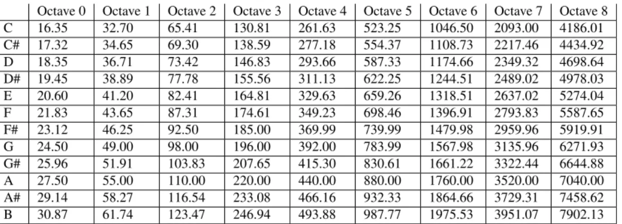
Table 2.1: The scientific pitch notation (SPN) for pitches, assigns a frequency to each pitch in a specific octave.

Octave 0 Octave 1 Octave 2 Octave 3 Octave 4 Octave 5 Octave 6 Octave 7 Octave 8

C 16.35 32.70 65.41 130.81 261.63 523.25 1046.50 2093.00 4186.01 C# 17.32 34.65 69.30 138.59 277.18 554.37 1108.73 2217.46 4434.92 D 18.35 36.71 73.42 146.83 293.66 587.33 1174.66 2349.32 4698.64 D# 19.45 38.89 77.78 155.56 311.13 622.25 1244.51 2489.02 4978.03 E 20.60 41.20 82.41 164.81 329.63 659.26 1318.51 2637.02 5274.04 F 21.83 43.65 87.31 174.61 349.23 698.46 1396.91 2793.83 5587.65 F# 23.12 46.25 92.50 185.00 369.99 739.99 1479.98 2959.96 5919.91 G 24.50 49.00 98.00 196.00 392.00 783.99 1567.98 3135.96 6271.93 G# 25.96 51.91 103.83 207.65 415.30 830.61 1661.22 3322.44 6644.88 A 27.50 55.00 110.00 220.00 440.00 880.00 1760.00 3520.00 7040.00 A# 29.14 58.27 116.54 233.08 466.16 932.33 1864.66 3729.31 7458.62 B 30.87 61.74 123.47 246.94 493.88 987.77 1975.53 3951.07 7902.13

An octave is the distance between a musical pitch and another with half or double its frequency. The octave relationship is important for our perception of music, because the human ear tends to hear two pitches at distance of one or more octaves, as being essentially the same pitch.

The equal temperament system divides each octave in 12 pitches, with the formula:

fp = 21/12fp−1 (2.1)

Pitches can be labeled using a combination of letters and numbers, as in scientific pitch notation, that assigns a frequency to each pitch in a specific octave (Table 2.1).

The terms pitch, tone and note are used as synonyms throughout this thesis.

2.1.2 Scale and Intervals

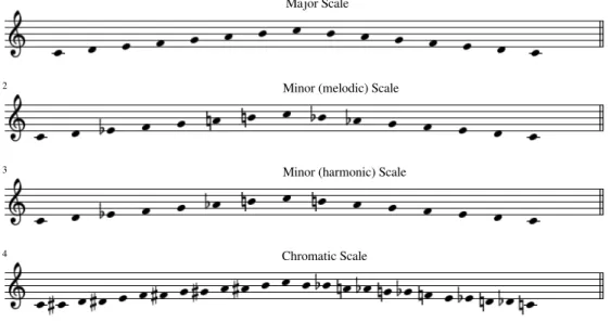
A sequence of ordered pitches is called a scale. Two scales are used as the basis of Western music: major scale and minor scale (with its harmonic and melodic forms) [53]. Another important scale is the chromatic scale, characterized by the fact that it is an ordered sequence of all the pitches. When the utilization of a particular scale is defined (or implicitly given from the context), it is common to refer to each step of the scale with the term degree. For example, in the major scale of Figure 2.1, the F note is called "fourth degree", since it is the forth note of the scale from the tonic. Scale degrees are often notated using roman numbers.

The basis of harmony is the interval. This name is used to describe the "distance" between the two tones, measured by their difference in pitch. If the two tones are not heard at the same time, but are consecutive tones of a melody, the interval is called a melodic interval, as distinguished from the harmonic interval in which the two tones are sounded together (Figure 2.2).

The smallest music interval is called semitone (a.k.a. half step or half tone) and it is defined as the interval between two adjacent notes in a chromatic scale. Two semitones form a tone. The bigger intervals can be defined using the ones founding the major scale

(21)

2.1. Tonal Harmony 2 3 4 Major Scale Minor (melodic) Scale Minor (harmonic) Scale Chromatic Scale

Figure 2.1: The most used scales in Western music: major scale, minor scale (with its harmonic and melodic forms), and chromatic scale.

Melodic Interval Harmonic Interval

(22)

5 perf. unison maj second maj third perf. fifth perf. fourth maj sixth maj seventh maj ninth perf. octave

Figure 2.3: The common names used for the intervals between the starting note of a major scale and the other notes.

Table 2.2: The most used interval labels in music theory with the corresponding number of semitones. Interval Name Note Example # of Semitones

unison C - C 0 aug. unison C - C# 1 min. 2nd C - Db 1 maj. 2nd C - D 2 aug. 2nd C - D# 3 min. 3rd C - Eb 3 maj. 3rd C - E 4 aug. 3rd C - E# 5 perf. 4th C - F 5 aug. 4th C - F# 6 dim. 5th C - Gb 6 perf. 5th C - G 7 aug. 5th C - G# 8 min. 6th C - Ab 8 maj. 6th C - A 9 aug. 6th C - A# 10 min. 7th C - Bb 10 maj. 7th C - B 11 octave C - C 12

as a reference; they can be defined in term of semitones or tones, but it is common in music theory to refer to them with another notation (Figure 2.3). Among the intervals from the major scale, the second, the third, the sixth and the seventh are said major; Octave, fifth, fourth and unison are instead defined with the term perfect. If the upper tone does not coincide with a note of the scale, the following considerations are to be applied:

• An interval a half-tone smaller than a major interval is minor.

• An interval a half-tone larger than a major or perfect interval is augmented. • An interval a half-tone smaller than a minor or a perfect interval is diminished. From the Table 2.2 it is possible to see that it often happens that two intervals with a different name correspond to the same number of semitones. A good example is the augmented second, which cannot be distinguished from the minor third, without further evidence than the sound of the two tones. In this situation, one interval is called the enharmonic equivalent of the other. Explaining the reason why different names are necessary for the enharmonic equivalent intervals is beyond the purpose of this small introduction.

(23)

2.1. Tonal Harmony

13

maj. 6th minor 3rd

Figure 2.4: The harmonic inversion of a major sixth. This operation can change the name of the interval.

Root Position fifth third root First Inversion root fifth third Second Inversion third root fifth

Figure 2.5: The three possible inversions of a triads. It is possible to still uniquely identify the note generated by the superposition if third, using the names "root", "third" adn "fifth".

In this procedure the names of the notes remain the same, but the lower of the two becomes the upper (or vice versa) with the consequence that there is usually a change in the name of the interval (Figure 2.4).

2.1.3 Triads

A Chord is the superposition of two or more intervals. The simplest chord is the triad, a chord of three tones obtained by the superposition of two thirds. The triad is the basis of the Western harmonic system. The names root (or fundamental), third and fifthare given to the three tones of the triad. These terms allow to identify the tones even if the notes can be duplicated at different octaves or rearranged in a different order (Figure 2.5).

A triad with its root as its lowest tone is said to be in root position. A triad with its third as its lowest tone is said to be in the first inversion. A triad with its fifth as its lowest tone is said to be in the second inversion. Changing the lowest note is an operation that can change the way it is perceived. There are other possible operations that can be performed on the notes of a triad; for example it is possible to move notes or duplicate them at different octaves, giving us a lot of possible ways of playing the same chord.The specific way the notes of a chord are assembled is called voicing.

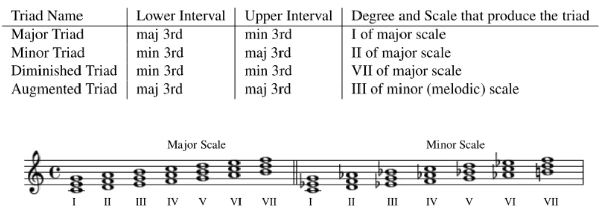
Taking the scales, major and minor and using only the notes of these scales, superpo-sition of third gives triads that differ depending on the kind of third in their make-up (Figure 2.6). This process is called harmonization of the scale. There are four kinds of triads, classified according to the nature of the intervals formed between the root and the third and between the third and the fifth. In the Table 2.3 we specify the intervals for each triad and we give an example of the scale and the degree that generate each type of triad.

Roman numbers identify not only the scale degree, but also the chord constructed upon that scale degree as a root. More details on the chord notation are in the Sub-section 2.1.5

(24)

Table 2.3: The four kinds of triads, classified according to the nature of the intervals formed between the root and the third and between the third and the fifth.

Triad Name Lower Interval Upper Interval Degree and Scale that produce the triad Major Triad maj 3rd min 3rd I of major scale

Minor Triad min 3rd maj 3rd II of major scale Diminished Triad min 3rd min 3rd VII of major scale

Augmented Triad maj 3rd maj 3rd III of minor (melodic) scale

III II

I IV V VI VII I II III IV V VI VII

Major Scale Minor Scale

Figure 2.6: Harmonization of major and minor (harmonic) scale.

2.1.4 Chords with 4 or more notes

Once a triad is built, it is easy to extend it by superimposing another third. This is the most used way of creating chords with 4 notes. The chord so produced is called seventh chord, and the added note is called seventh. This kind of chord is widely used in jazz music, along with chords of 5, 6 and 7 notes. The number of possible combinations of thirds explodes while we add notes. However, since in this thesis we deal mainly with pop music, we consider a single seventh chord, called dominant seventh chord. It is built on the V degree of the major or minor scale and it is composed by the superposition of a major third and two minor thirds (Figure 2.7).

The operations on the triads (inversion of the chords and duplication of some notes) can be performed in the same way on the chords with 4 or more notes. In case of seventh chords, there are 3 possible inversions.

2.1.5 Harmonic Progression

Music can be considered as a temporal evolution of many musical parameters. It is common to refer to sequences of chords during a song as harmonic progressions. There are two common notations for chord progressions:

1. Sequences of pairs (root name, chord type). For example D - E:min - G - A:min. 2. Sequences of scale degrees, indicated by roman numbers (where the current scale

must be defined explicitly). For example I-II-V-VI in the scale of D major.

Dominant Seventh

(25)

2.2. Mathematical Background The two notations have different advantages. The first notation allows to absolutely define a chord without needing further information about the musical context. It is the most simple notation and for this reason is widely adopted for jazz and modern music. The second notation, on the contrary, requires some experience in music theory, to understand exactly the kind of chord (minor, major, etc.) that is built on the specific root using the notes of the scale. This notation is useful for the analysis, since it is "pitch independent", i.e. it can be transposed to higher or lower pitches, by simply changing the scale of reference.

In tonal harmony different chords have different degrees of perceived stability. I is the most stable chord and V is the most unstable. Consequently each chord in a progression is invested with a particular role, called harmonic function. The basic chord progres-sion is built starting from a stable chord, evolving towards more unstable chords and returning in the end to the stable chord.

There are many guidelines about how to manage harmonic progressions. For a com-plete discussion on this subject, we suggest [53] for classical/pop music and [38] for jazz music.

We saw in section 2.1.3 that there are many possible voicings for a chord. The way the different notes of chord voicings are connected in a progression is an import task in music composition, because it has a big impact on the way harmonic progressions are perceived. The study of this field is called counterpoint.

2.2

Mathematical Background

In this section we give some basic concepts of probability theory, information theory and machine learning that will be useful to understand the techniques that we will use for the generation of harmonic progressions.

2.2.1 Probability Theory

Probability theory is a mathematical framework for representing uncertain statements. It provides a mean for quantifying uncertainty, and axioms for deriving new uncer-tain statements. Nearly all activities require some ability to reason in the presence of uncertainty. In fact, beyond mathematical statements that are true by definition, it is difficult to think of any proposition that is absolutely true or any event that is absolutely guaranteed to occur.

There are three possible sources of uncertainty [20]:

1. Inherent stochasticity in the system being modeled. For example most interpreta-tions of quantum mechanics describe the dynamics of subatomic particles as being probabilistic. It is also possible to create theoretical scenarios that we postulate to have random dynamics, such as a hypothetical card game where we assume that the cards are truly shuffled into a random order.

2. Incomplete observability. Even deterministic systems can appear stochastic when we cannot observe all of the variables that drive the behavior of the system. For

(26)

example, the behavior of a person who chooses to go outside or to stay at home depending on the weather, would seem stochastic, if it is not possible to observe the weather.

3. Incomplete modeling. When one uses a model that must discard some of the in-formation observed, the discarded inin-formation results in uncertainty in the model prediction. For example, let us consider a robot that can exactly observe the lo-cation of every object around it. Since it has to discretize the space to save the information, the position of the objects for the robot become uncertain within the discrete cell.

A random variable is a variable that can take on different values randomly. It can be discrete or continuous. A discrete random variable is one that has a finite or countably infinite number of states. A continuous random variable is associated with a real value. In this thesis we will work with discrete random variables, since the events that we consider (chords, voicing, etc...) have a countable number of possibilities.

A probability distribution is a description of how likely a random variable or set of ran-dom variables is to take on each of its possible states. A probability distribution over discrete variables may be described using a probability mass function (PMF). Specifi-cally, a PMF maps from a state of a random variable to the probability of that random variable taking on that state. For example p(z = x) defines the probability for the ran-dom value z to be equal to the value x. If the ranran-dom value z we are referring to can be deduced from the context, we will write p(x) to simplify the notation. Probability mass functions can act on many variables at the same time. Such a probability distributon over many value is known as a joint probability distribution p(z = x, v = y). Again we will write p(x, y) for brevity when the dependency on z and v is evident from the context. An example of PMF that we will use frequently is the uniform distribution over a discrete random variable z with k different states x1, x2, ..., xk:

p(z = xi) = p(xi) =

1

k, for i from 1 to k (2.2)

Sometimes it is known the probability distribution over a set of variables and one wants to know the probability distribution over just a subset of them (Figure 2.8). This value is known as the marginal probability distribution. For example, if there are discrete random variables z and v that can take values respectively from X = x1, x2, ... and

Y = y1, y2, ... and p(x, y) is known, it is possible to find p(x) with the sum rule:

∀x ∈ X, p(z = x) =Xy ∈ Y p(z = x, v = y) (2.3)

In many cases it is interesting to to know the conditionl probability, i.e. the probability of an event x, given that another event y has happened. It is denoted as p(x|y). A useful formula that relates conditional and joint probability is:

p(y|x) = p(y, x)

p(x) , if p(x) > 0 (2.4)

An extension of the equation 2.4 is the so called chain rule. It considers a probabil-ity distribution over n random variables and explains how it can be decomposed into

(27)

2.2. Mathematical Background 3 2 1 0 1 2 3 X1 3 2 1 0 1 2 3 X2

Figure 2.8: The two marginal probabilities of a joint probability distribution of two variables p(X1, X2),

obtained with the sum rule.

conditional distributions over only one variable:

p(x1, ..., xn) = p(x1) n

Y

i=2

p(xi|x1, ..., xi−1) (2.5)

Two random variables x and y are independent if their probability distribution can be expressed as a product of two factors, one involving only x and one involving only y:

p(x, y) = p(x)p(y) (2.6)

Two random variables x and y are conditionally independent given a random variable z if the conditional probability distribution over x and y can be factorize as follows:

p(x, y|z) = p(x|z)p(y|z) (2.7)

The expectation or expected value of a function f (x) with respect to a probability dis-tribution p(x) is the average value that f takes on when x is drawn from p(x). For discrete variables this can be computed with a summation:

E[f (x)] = X

x

p(x)f (x) (2.8)

The variance gives a measure of how much the values of a function of a random variable x vary, as different values of x from its probability distribution are sampled:

(28)

When the variance is low, the values of f (x) cluster near their expected value.

The covariance gives some sense of how much two values are linearly related to each other, as different values of x from its probability distribution are sampled:

Cov(f (x), g(x)) = E[(f (x) − E[f (x)])(g(y) − E[g(y)])] (2.10) High absolute values of the covariance mean that the values greatly change and are both far from their respective means simultaneously. If the sign of the covariance is positive, then both variables tend to take on relatively high values simultaneously. If the sign of the covariance is negative, then one variable tends to take on a relatively high value and the other takes on a relative low value.

Correlation is another measure that normalizes w.r.t. the scale of both variables, re-sulting in a bounded coefficient [−1, 1]. Two kinds of correlation used in statistics are Pearson Correlation and Spearman Correlation. Pearson correlation evaluates the linear relationship between two variables, while Spearman correlation assesses how well an arbitrary monotonic function can describe a relationship between two vari-ables [26].

2.2.2 Information Theory

Information theory is a branch of applied mathematics that revolves around quantifying how much information is present in a signal . It was originally invented to study send-ing messages with a discrete alphabet over a noisy channel, such as communication via radio transmission. The basic intuition behind information theory is that learning that an unlikely event has occurred is more informative than learning that a likely event has occurred. For example a message saying "the sun rose this morning" is so uninforma-tive as to be unnecessary to send, but a message saying "there was a solar eclipse this morning" is very informative [20]. Information theory quantifies information in a way that formalizes this intuition. Specifically:

• Likely events should have low information content (or no information content if the events are guaranteed to happen)

• Less likely events should have higher information content.

• Independent events should have addictive information. For example, if finding out that a tossed coin has come up as heads conveys a certain information x, finding out that it has come up as head twice should convey an information 2x.

The self-information of an event x is defined with a formulation that satisfies all these properties:

I(x) = − log p(x) (2.11)

The choice of the base of the logarithm is not really important, however a common choice is to use base 2 logarithm. In this case information I(x) is measured in bits. Self-information deals only with a single outcome. It is possible to quantify the amount of uncertainty in an entire probability distribution using the Shannon Entropy:

(29)

2.2. Mathematical Background Distributions that are nearly deterministic have a low entropy, while distributions that are closer to the uniform have high entropy.

If one has two separated probability distributions p(x) and q(x) over the same random variable x, it is possible to measure how different these two distributions are, using the Kullback-Leibler (KL) divergence:

DKL(p k q) = E[log

p(x)

q(x)] = E[log p(x) − log q(x)] (2.13) The KL divergence is non-negative and it is 0 if and only if p and q are the same distribution.

A quantity that is closely related is the cross-entropy. For two distributions q and p, it measures the average number of bits needed to identify an event drawn from the set, if a coding scheme is used that is optimized for the distribution p, rather than the "true" distribution q. For discrete p and q it can be written as:

H(q, p) = −X

x

q(x) log p(x) (2.14)

Unfortunately for many applications, like the estimation of the regularity of the models used in this thesis, the distribution q is unknown. In these cases, a typical approach is to use a Monte Carlo estimation of the true cross entropy [14]:

Hp(T ) = − 1 |T | X x∈T log₂p(x) (2.15) 2.2.3 Graphical models

Machine learning algorithms often involve probability distributions over a very large number of random variables. In order to reduce the complexity it is possible to split a probability distribution into a product of many factors. For example, let us suppose we have three random variables: a, b and c; let us suppose also that a influences the value of b and b influences the value of c, but a and c are independent given b. It is possible to represent the probability distribution over all three variables as a product of probability distributions over two variables:

p(a, b, c) = p(a)p(b|a)p(c|b) (2.16)

This kind of factorization can greatly reduce the number of parameters needed to de-scribe the distribution. Since each factor uses a number of parameters that is expo-nential in the number of variables in the factor, one can greatly reduce the cost of representing a distribution if one is able to find a factorization into distributions over fewer variables [14]. It is possible to describe this kinds of factorizations using directed acyclic graphs. The factorization of a probability distribution, represented with a graph, is called Graphical Models (Figure 2.9).

When one applies a graphical model to a problem in machine learning or pattern recog-nition, one will typically set some of the random variables to specific observed values,

(30)

Figure 2.9: A graphical model representing the probability distribution defined in the equation 2.16. The node represents the random variables and the arrows represent a variable conditioning another variable

i.e. variables whose value is known. We denote such variables by shadowing the cor-responding note.

Let us study the particular case of Figure 2.10, in order to derive some results that we will use later. By applying twice the chain rule 2.5 we obtain:

p(a, b, c) = p(a)p(c|a)p(b|c) (2.17)

In the model (a), where none of the nodes is observed, if we test if a and b are indepen-dent, we obtain (marginalizing over c):

p(a, b) = p(a)X

c

p(c|a)p(b|c) = p(a)p(b|a) = p(a)p(b|a) (2.18)

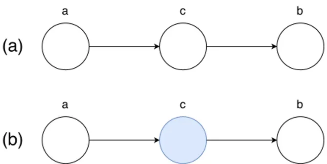
which in general does not factorize into p(a)p(b), so a and b are not independent. If instead we consider the model (b), where the node c is observed, we obtain:

p(a, b|c) = p(a, b, c) p(c) = p(a)p(c|a)p(b|c) p(c) = p(a|c)p(b|c) (2.19)

from which we obtain the conditional independence property of a and b given c. The path from a to b is said to be blocked by the observed node c.

2.2.4 Machine Learning Basics

The field of machine learning is concerned with the question of how to construct com-puter programs that automatically learn from experience [45]. Mitchell suggests also a more precise definition for the concept of learning.

Definition 2.1. A computer program is said to learn from experience E with respect to some class of tasksT and performance measure P , if its performance at task in T , as measured byP , improves with experience E.

(31)

2.2. Mathematical Background

Figure 2.10: Two different graphical models. The shadowed node in (b) represents an observed node.

For example, it can be considered a machine learning system for handwriting recogni-tion. In this case, the task T would be of recognizing and classifying handwritten words within images; the performance measure P would be the percentage of word correctly classified; the training experience E would come from a database of handwritten words with given labels.

The following sections provide an intuitive description and some examples of the differ-ent kinds of tasks, performance measures and experiences that can be used to construct a machine learning algorithm.

The Task, T . Machine learning allows us to tackle tasks that are difficult to solve with fixed programs written by human beings. Tasks are usually described in terms of how the machine learning system should process an input, i.e. a collection of features that have been quantitatively measured from some objects or events. We typically represent the input as a vector x ∈ Rn, where each element xi is a feature. The machine learning

tasks can be clustered into three big groups:

• Classification: the computer is asked to specify which of k categories some inputs belongs to. This is usually accomplished by assigning to each input feature vector x a class from the k possible output classes (or a probability distribution over the output classes). A typical example is the handwriting recognition, where the input are the pixel of an image and the output is a letter from the alphabet.

• Regression: the computer is asked to predict a numerical value given some inputs. To solve this task, the learning algorithm is asked to output a function f : Rn→ R. An example of a regression task is the prediction of the value of a house, given a set of features such as the location, the number of rooms, the age and other factors. • Clustering: the computer is asked to find a structure in a collection of unlabeled inputs. In other words, the task consists in organizing inputs into groups whose members are similar in some way. The exact meaning of "similar" or "dissimilar" inputs can change between different clustering algorithms. An example of clus-tering task can be to find similar groups of pixel in an image, in order to better perform image compression.

The Experience, E. The machine learning algorithms need a dataset of elements to be used as input. We call these elements data points. Usually, the bigger the dataset is,

(32)

the better the algorithm will accomplish its task; however there are algorithms that are made on purpose to work properly with bigger or smaller datasets. Machine learning algorithms can be broadly categorized a supervised and unsupervised by what kind of experience they are allowed to have during the learning process. "Supervised" means that both input and output are given, and the algorithm must learn the rules that relate an input with the corresponding output. In unsupervised learning only the inputs are given and the algorithm uses them to build an high-level representation of the data. For the purpose of this thesis, we will consider only supervised learning.

Performance Measure, P . In order to evaluate the abilities of a machine learning algo-rithm, quantitative measure of its performance must be designed. For the classification tasks, it is often measured the proportion of the input data for which the model pro-duces the correct output. It is possible also to obtain similar results by measuring the proportion of input data that generates an incorrect output. The choice of performance measure is not straightforward. For example [14], when performing a transcription task, should we measure the accuracy of the system at transcribing entire sequences, or should we use a more fine-grained performance measure that gives partial credit for getting some elements of the sequence correct? When performing a regression task, should we penalize the system more if it frequently makes medium-sized mistakes or if it rarely makes very large mistakes? These kinds of design choices depend on the application.

Underfitting and Overfitting

In order for a machine learning algorithm to give meaningful results, it must perform well on previously unseen inputs, different from the inputs used to train the algorithm. Typically, a training set is available, and the training error can be reduced as an op-timization process over the model parameters. What separates machine learning from simple optimization is that the error, generated by test data (data not used for train-ing) must be low as well. The test error of a machine learning model is estimated by measuring its performance on a test set of inputs that were kept separate from the training set. The problem of improving the performances on the test set, if only the training set is observed, requires more assumptions to be solved: the train and test data must be considered as independent and identically distributed, generated by the same probability distribution (i.i.d. assumption).

With this notions it is possible to define the two central problems of machine learning: underfittingand overfitting. Underfitting occurs when the model is not able to obtain a sufficiently low error value on the training set. Overfitting occurs when the gap between the training error and the test error is too large. It is possible control whether a model is more likely to overfit or underfit by altering its flexibility, i.e. its ability to fit a variety of functions. Models with low flexibility may struggle to fit the training set and are not able to solve complex tasks. Models with high flexibility are prone to model noise and errors in the dataset that should not be part of the model. So we must carefully choose the right model flexibility. Unfortunately there is not a right choice for every dataset. The No Free Lunch Theorem [64] states that, averaged over all possible data

(33)

2.2. Mathematical Background generating distributions, every classification algorithm has the same error rate when classifying previously unobserved data points. In other words, the most sophisticated algorithm that can be conceived has the same average performance (over all possible tasks) as a toy predictor that assigns all data points to the same class. This means that the goal of machine learning research is not to seek a universal learning algorithm or the absolute best learning algorithm. Instead, its goal is to understand what kind of distributions are relevant to the "real work" and what kinds of machine learning algorithms perform well on data drawn from the kinds of data generating distributions that are considered [20].

Regression Analysis

Regression analysis is one of the three tasks mentioned above. We provide here further details, since we will extensively use it in Chapter 4.

Suppose that for each value of a quantity x, another quantity y has a probability distri-bution p(y|x). The mean value of this distridistri-bution, alternatively called the expectation of y, given x, and written E(y|x), is a function of x and is called the regression of y on x. The regression provides information about how y depends on x [39]. The quanti-ties x and y are respectively called independent variable and dependent variable. The simplest case is linear regression, where E(y|x) = ω1x + ω0 for parameters ω1 and

ω0. In case of polynomial regressions, the relationship between x and y is modeled as

a nth degree polynomial in x. This can be seen in an informal way as a problem of curve fitting. In particular, one shall fit the data by using a polynomial function of the form: y(x, ω) = ω0+ ω1x + ω2x2+ ... + ωMxM = M X j=0 ωjxj (2.20)

The values of the coefficients are determined by fitting the polynomial to the training set. This can be done by minimizing an error function that measures the misfit between the function y(x, ω), for any given values of omega and the training set data points [7]. One simple choice of error function is given by the sum of squares of the errors between the predictions y(xn, ω) for each data point xnand the corresponding target values tn,

so that we minimize E(ω) = N X n=1 (y(xn, ω) − tn)2 (2.21)

This technique is called least-square estimation.

Robust Regression

Least-square estimation has bad performances when the error distribution is not nor-mal, particularly when the errors are heavy-tailed [19]. In these situations there is the necessity to use another fitting criterion that is not as vulnerable as least-squares to outliers.

A possibility is to use the Huber function as error function. In contrast to the least-square function, Huber function assigns a weight to each observation, that declines

(34)

when |e| > k. The value k affects the performances of the regression: smaller values produce more resistance to outliers, but at the expenses of lower efficiency when the errors are normally distributed. Usually k is chosen as k = 1.345σ (where σ is the standard deviation of the errors), since it produces 95-percent efficiency when the errors are normal, but still offers protection against outliers.

2.3

Related Work

The analysis of the relation between complexity and preference rating is not a particu-larly investigated field within the MIR community. Some works in this direction came from the field of psychology, and we present them in Section 2.3.1.

Then, we propose studies about the analysis of harmonic complexity and studies that consider perceptual descriptors such as "stability", "degree of completeness", "experi-enced tension", "music expectation", that can be considered related to our definition of harmonic complexity.

Lastly, we present also works that inspired the methodology for modeling of chord sequences, the analysis of the results and the design of the listening test.

2.3.1 Complexity and preference

In [2], Berlyne repetitively proposes to a subject black and white reproductions paint-ings with different levels of complexity: more complex paintpaint-ings (crowded canvases with many human figures), less complex paintings (portraits of a single person), more complex nonrepresentational patterns (containing many elements), and less complex nonrepresentational patterns. He observes that, with repeated exposition, the less com-plex pictures were rated significantly more and more displeasing, while the ratings for the more complex pictures did not change significantly.

In [59], Skaife shows that preference tends, when "simple" popular music is presented, to decline with increasing familiarity. But with repetitive hearing of jazz, classical, or contemporary music that violates traditional conventions, there is normally a rise followed by a decline. Similar results were reached by Alpert [1] with rhythmic pat-terns.

In [3], Berlyne proves that the individual’s preference for a certain piece of music is related to the amount of activity it produces in the listener’s brain, which he refers to as arousal potential. In particular, there is an optimal arousal potential that causes the maximum liking, while a too low as well as a too high arousal potential results in a decrease of liking. He illustrates this behavior by an inverted U-shaped curve (Figure 1.2).

In [8], two groups of twenty college students, one with fewer than two years of musical training and the other with extensive musical backgrounds, rated their preferences for piano recordings of J.S. Bach’s "Prelude and Fugue in C Major", Claude Debussy’s "The Maid With the Flaxen Hair", Edvard Grieg’s "Wedding Day at Troldhaugen", and

(35)

2.3. Related Work Pierre Boulez’s "Piano Sonata No.1, 2nd Movement". Each piece had been ranked ac-cording to perceived complexity by seven music professors. When personal preference was plotted against complexity, an inverted U-shape curve was obtained.

2.3.2 Model-Based Symbolic analysis of Chord Progressions

One of the most intuitive approach is to analyze chord progressions, by trying to define explicitly the instinctive steps that a trained musician would perform. Therefore these techniques exploit knowledges and rules from music theory and propose algorithms to evaluate human perception of complexity and similarity.

In [41] [42], the authors propose a mathematical model based on Tonal Harmony (TH), in order to be able to use high level harmonic features in computer systems applications. In particular, they consider the harmony like a formal grammar, with some transforma-tion rules between chords taken from music theory. If music obeys simple TH rules, they assign it a lower value, whereas if the rules are complex, or the harmony does not obey any known rules, they assign it higher values. The values of each chord transition are then combined and they define a new term, harmonic complexity. This feature is then tested on a music classification problem, proving that it is useful for Music Infor-mation Retrieval tasks.

Hanna et al. [25] in his Chord Sequence Alignment System (CSAS), compute the sim-ilarity value between two different chord sequences with an algorithm based on align-ment. The similarity is computed with the recursive application of only three transfor-mation rules: deletion of a symbol, insertion of a symbol, and substitution of a symbol by another. Each transformation has its own cost and, while the insertion and deletion costs are equal and constant, different functions for the substitution score (related to the roots, the basses, the types, the modes of the two chords) are proposed and com-pared.

De Haas [40] [16] presents a formalization of the rules of harmony as a Haskell (gener-alized) algebraic datatype. The Haskell advanced type system features make it possible to use datatype-generic programming to derive a parser automatically. Thus, given a sequence of chord labels, it is possible to derive a tree structure, which explains the har-monic function of the chords in the piece. The number of errors in creating the tree or the tree depth can be considered as a possible way to calculate the harmonic complexity by using tonal harmony, even though it was not the aim of the work. This system is then used on a corpus of 217 Beatles, Queen, and Zweieck songs, yielding to a statistically significant improvement for the task of machine chord transcription [15].

An interesting MIR system is the one developed by Pickens and Crawford [52] in order to retrieve polyphonic music documents by polyphonic music queries. The idea can be summarized in two steps. In the first part they preprocess the music score of each docu-ment in the collection in order to obtain a probability distributions over all chords, one for each music segment. In other words, instead of extracting chord labels from each score segment, they extract a 24 dimensional vector describing the similarity between the segment and every major and minor triad. In the second part they apply Markov modeling techniques, and store each document as a sequence of transitions (computed

(36)

with a fixed-order Markov Model) between these 24 dimensional vectors. Queries are then modeled using the same modeling technique of the documents and the Kullback-Leibler divergence is used as a ranking system to obtain the most similar document for the query.

2.3.3 Data-based Symbolic Analysis of Chord Progressions

Another possible approach is to put aside the prior knowledge from music theory and instead working with big dataset of annotated symbols (e.g. chords sequence or scores) in order to extract the rules that control music perception. This way of acting is sup-ported by some psychology research [35] that pointed out that listeners appear to build on a set of basic perceptual principles that may adapt to different styles, depending on the kind of music they are exposed to.

In [63], the authors use multiple viewpoint systems and Prediction by Partial Match-ing to solve the problem of automatic four-part harmonization in accordance with the compositional practices of a particular musical era.

In [55], Rohrmeier et al. compare the predictive performance of n-gram, HMM, autore-gressive HMMs, feature-based (or multiple-viewpoint) n-gram and Dynamic Bayesian Network Models of harmony. All this models use a basic set of duration and mode features. The evaluation is performed by using a hand-selected corpus of Jazz stan-dards.

In [49], the authors propose to use a statistical-based data compression approach to infer recurring patterns from the corpus and show that the extracted patterns provide a satis-fying notion of expectation and surprise. After this unsupervised step, they exploit the underlying algebra of Jazz harmony, represented as chord substitution rules, but they extract those rules from the dataset. The results prove that data-inferred rules corre-spond, in general, to the usual chord substitution rules of music theory textbooks. In [58], the authors model chord sequences by probabilistic N-grams and use model smoothing and selection techniques, initially designed for spoken language modeling. They train this model with a dataset composed by 14194 chords from the 180 songs making up the 13 studio albums of The Beatles.

2.3.4 Mixed Symbolic Analysis of Chord Progressions

Paiement et al. [50] propose a work that use both the data-based and the model-based approach. They define a distributed representation for chords that gives a measure of the relative strength of each pitch class, taking into account not only the chord notes, but also the perceived strength of the harmonics related to every note (where the amplitude of the harmonics is approximated with a geometric decaying variable. This representa-tion has the effect that the Euclidean distance between chords can be used as a rough measure of psychoacoustic similarity. In the second part of the paper the authors present a probabilistic "three shaped" graphical model of discrete variable, with three layers of hidden nodes and one of observed nodes (Figure 2.11). This structure can model chord progressions by considering different levels of context: variables in level 1 model the

(37)

2.3. Related Work

Figure 2.11: A probabilistic graphical model for chord progressions. Numbers in level 1 and 2 nodes indicate a particular form of parameter sharing [Figure taken from [50]]

contextual dependencies related to the meter, in level 2 local dependencies are taken into account and in level 3 it is used the distributed chord representation in order to substitute chords with "similar" chords. This last step gives a solution to the problem of unseen chords, since it just considers the "similar" chords to redistribute efficiently a certain amount of probability mass to those new events. This model is trained by using a dataset of 52 jazz standards; from the results it is possible to see that the three model performed better, compared with a standard HMM model trained on the same data.

2.3.5 Harmonic Complexity from Audio

Instead of starting from a symbolic representation, another approach is to use directly audio features.

In [44], the authors define a new meta-feature, Structural Change, that can be calculated from an arbitrary frame-wise basis feature, with each element in the structural change feature vector representing the change of the basis feature at a different time scale. Then they conducted a web-based experiment whose results suggest that the proposed feature correlates with the human perception of change in music. The relationship of structural change with complexity is hypothesized but left for future work.

In [62], the authors consider Beethoven’s Sonatas and proceed to analyze harmonic complexity on different levels: chord level, fine structure, coarse structure, cross-work and cross-composer. Three different features are taken into account: Shannon entropy of the chroma vector, the quotient between the geometric and the arithmetic mean of the chroma vector, and harmonic similarity of the pitch classes computed on a reordered chroma vector to a perfect fifth ordering.

(38)

Figure 2.12: The result of the probe tone experiment for C major and A minor keys. Listeners rated how much the specific tone sounds conclusive [Figure taken from [36]].

2.3.6 Cognitive Approach to Music Analysis

Different contributions on how tonal organization affects the way music is remembered come from the field of psychology.

One of the first experiments is the probe tone technique, proposed by Krumhansl and Shepard [33], in order to quantify the hierarchy of tonal stability. In this study, an in-complete C major scale (without the final tonic, C) is sounded in either ascending or descending form in order to fix in the listener the perception of the C major key. The scale is then followed by one of the tones of the next octave (the probe tone). This experiment is repeated for every tone of the chromatic scale and the listener has to rate how well each tone completed the scale. The more musically trained listeners pro-duced a pattern that is expected from music theory: the tonic was the most rated tone, followed by the fifth, third, the remaining scale tones, and finally the nondiatonic tones (Figure 2.12). In [36], Krumhansl and Kessler extend this method by using chord ca-dences and both major and minor scales as a context. A similar experiment [34] was conducted with the first movement of Mozart’s piano Sonata K.282. The listeners had to adjust an indicator on the computer display to show the degree of experienced ten-sion. The task was designed to probe three aspects of music perception: segmentation into hierarchically organized units, variations over time in the degree of experienced tension, and identification of distinct musical ideas as they are introduced in the piece. A deepening in this field can be found in [34].

In [5], the authors perform three listening tests to investigate the effect of global har-monic context on expectancy formation. Among the other results they demonstrate that global harmonic context governs harmonic expectancy and that neither an explicit knowledge of the Western harmonic hierarchy nor extensive practice of music are re-quired to perceive small changes in chord function.

(39)

CHAPTER

3

Modeling Chord Progressions

T

HEeasiest way to treat chord progressions would be simply to ignore the

sequen-tial aspects and to treat the observations as independent identically distributed (i.i.d.). The only information we could glean from data would be, then just the relative frequency of every single chord. However, if we consider tonal harmony rules, we can find out, for example, that after a dominant chord it is highly probable to find a tonic chord; or that after the sequence I − II we can expect a dominant chord. Ob-serving the previous chords is therefore of significant help in predicting the following chord.

We call this kind of data sequential data [7]. These are often produced through mea-surement of time series, for example the rainfall meamea-surement on successive days at a particular location, the acoustic features at successive time frames used for speech recognition or, in this thesis, the chord sequence in a song.

It is useful to distinguish between stationary and non-stationary sequential distribu-tions. In the stationary case, the data evolves in time, but the distribution from which it is generated remains the same. For the more complex non-stationary situation, the generative distribution itself is evolving with time. However, we will model the the rules for chord sequences generation as stationary, so here we consider only stationary sequential distributions.

To model the probability of a chord given the sequence of the previous chords

p(xi|xi−1, xi−2..., xi−n), we choose to use three different models: Prediction by Partial