POLITECNICO DI MILANO
Facoltà di Ingegneria
Dipartimento di Elettronica, Informazione e Bioingegneria
A NEURO-FUZZY CONTROLLER FOR
SUPERCONDUCTING CABLE TESTING
RELATORE:
Prof. Ing. Cesare Svelto
CORRELATORE:
Prof. Ing. Pasquale Arpaia
TESI
DI
LAUREA
DI:
Vincenzo DAPONTE
matr.n. 755767
2
Index
Abstract
Acknowledgements Introduction
1. Monitoring systems for cable testing
1. Test station for superconducting cables 2. Test station monitoring
2. Gain Scheduling
1. Adaptive control
1. Main control approaches 2. Adaptive control strategies 2. Gain Scheduling
3. Fuzzy Gain Scheduling 4. Neuro-Fuzzy inference
1. Sugeno inference
2. Sugeno inference: network structure and learning 3. ANFIS inference
4. ANFIS inference: network structure and learning
3. Remote smart measurement system for superconducting cable test
1. The proposed system 2. Adaptive current control 3. Remote device interface
4. Neuro-fuzzy control system
1. Model Identification 2. Controller design
3. Neuro-Fuzzy strategy implementation
5. Remote control system
1. Requirements analysis
1. Front-end software architecture 2. Monitoring system 1. The Environment 2. The System 3. Logic Model 4. Functional requirements 5. Use Cases 2. System design
1. Monitoring system design and standards 1. Cycle definition
2. Status and errors definition 3. Classes design
4. Interaction flow 2. FESA Class design
6. Numerical Results
3 1. Measurements plan 2. Data analysis 3. Numerical results 2. System characterization 3. Model definition 4. Controller simulation 7. Experimental validation 1. Primary tuning 1. Measurements plan 2. State of the art comparison
Appendix Conclusions
4
Abstract
Superconductivity nowadays is finding more and more applications in addition to those strictly related to research and experimental physics. In particular, the critical current estimation plays a fundamental role in the characterization and usage of superconducting cables. At the European Organization for Nuclear Research (CERN) superconductivity is widely exploited in the development of particle accelerators such as the Large Hadron Collider (LHC). In this context the Facility for the Reception of Superconducting Cables (FReSCa) were created to perform test on superconducting cables and determine their properties in particular the critical current. There a measurement system based on a superconducting transformer and was introduced. The transformer different nonlinear behaviours showed led to a strategy for the transformer secondary current control resulted efficient under several constraints. Furthermore, the possibility to perform all tests only from the instrumentation rack computer does not allow the necessary view of all the relevant parameters to be monitored during a test session. The need for the measurement system to be integrated in the FReSCa control system together with the possibility to improve the current control performance resulted in the development of an integrated monitoring system. It provides the remote control of the measurement station and a control strategy that increases the performances with respect to the state of the art. Thus the proposed remote monitoring system for cable testing aims to allow the measurement system to be remotely driven through a CERN standardized remote device interface. Furthermore, it aims to overcome the limitations shown by the available measurement system related to the transformer secondary current control. The current control strategy was designed by following the Fuzzy Gain Scheduling logic which suggests changing in the controller parameters according to the working condition changes. The concrete implementation of the control logic was performed by means of a Neuro-fuzzy inference network.
5
Sommario
La Superconduttività al giorno d'oggi sta trovando sempre più applicazioni oltre a quelle strettamente connesse alla ricerca e alla fisica sperimentale. In particolare, la stima corrente critica gioca un ruolo fondamentale nella caratterizzazione e l'utilizzo di cavi superconduttori. Presso l'Organizzazione Europea per la Ricerca Nucleare (CERN) la superconduttività è ampiamente sfruttata per lo sviluppo di acceleratori di particelle come il Large Hadron Collider (LHC). In questo contesto, lo strumento per la Facility per i test su cavi superconduttori (FReSCa), è stata creati per eseguire i test su cavi superconduttori e determinare le loro proprietà, in particolare, la corrente critica. Un sistema di misura basato su un trasformatore superconduttore ed è stato introdotto recentemente. La dinamica non lineare mostrata dal trasformatore ha portato ad una strategia per il controllo della corrente sul secondario efficiente solo sotto diversi vincoli. Inoltre, la possibilità di eseguire tutti i test solo dal computer presente sul rack di strumentazione non consente la visualizzazione di tutti i parametri rilevanti durante una sessione di prova. La necessità che il sistema di misura debba essere integrato nel sistema di controllo a FReSCa insieme alla possibilità di migliorare le prestazioni del controllo di corrente hanno portato allo sviluppo di un sistema integrato di misura. Esso fornisce il controllo remoto della stazione di misura ed una strategia di controllo che aumenta le prestazioni della stazione rispetto allo stato dell'arte. Il sistema proposto vuole consentire al sistema di misura di essere guidato da remoto attraverso una interfaccia standard CERN per il controllo di dispositivi dispositivo remoti. Inoltre, si propone di superare i limiti indicati dal sistema di misura attuale relativi al controllo della corrente sul secondario del trasformatore. La strategia di controllo della corrente è stata progettata seguendo la logica Fuzzy Gain Scheduling che suggerisce di modulare i parametri del controllore in base ai cambiamenti delle condizioni di funzionamento. L'attuazione concreta della logica di controllo è stata effettuata per mezzo di una rete di inferenza Neuro-fuzzy.
6
Acknowledgements
A meno di un ora dalla consegna ufficiale di questo documento, faccio fatica a ricordare tutti coloro a cui debba e voglia dire almeno un “grazie”, non so se questo sia un bene perchè vuol dire che ho molti amici o un male perche vuol dire che ingnegneria fa davvero male come dicono. Sicuramente un grazie enorme per la disponibilitá e la pazienza lo porgo al prof. Svelto che mi ha aiutato in quest’ultima parte del mio cammino al Poli. Al prof. Arpaia non so davvero cosa dire, se prima ho detto grazie ora ci vorrá almeno un grazie infinite; ci siamo conosciuti in un modo molto tempo fa e ci siamo riconosciuti durante quest’esperienza (io non me lo ricordavo così). Un saluto ai miei amici di sempre Giovanni e Gino, presenze costanti e di grande supporto. Un grande in bocca a lupo voglio fare al Turco e signora con l’augurio di realizzare il loro sogno più grande. Un gigantesco grazie alla sorte per avermi fatto trovare due compagni di viaggio in una giungla, e uno a Francesco per la sua allegria e un altro enorme ad Alberto... lui sa per cosa. Un grande abbraccio voglio darlo a Chiara senza la quale sarei molto più scemo di quello che giá sono. Un pensiero affettuoso per il Direttore e signora che mi hanno accolto come fossi un rifugiato quando sbarcai a Milano e a Tonino per avermi fatto conoscere un’Italia che altrimeni non avrei mai visto. Un “cheers” ancora a tutti gli amici technical e all’Equipo C e agli amici italiani (G. e M. compresi) che hanno condiviso con me questo anno molto particolare. Un enorme grazie per tutto cio’ che mi hanno insegnato (non solo al lavoro) ai miei bodyguard della mente Lucio, Carletto, Giancarlo e il “Principale” più che un semplice capo. Un sincerro grazie a tre persone sincere come Robertone e Davidone e Andrea il presidente. Un fraterno grazie agli amici fraterni che ci sono sempre, anche quando non ci sono Francesco e Antonella. Oltre agli amici a Ginevra ho allargato anche la famiglia, ho acquisito due zie molto molto speciali, chi l’avrebbe mai detto! Mando un grande bacio ad entrambe.Il pensiero più profondo va alla famiglia, a quella lontana come i nonni, i miei angeli custodi, gli zii a Minori e a Roma in particolare va a Mamma e Papá perchè trovino la serenitá che meritano. A Sasha dico solo che gli voglio un bene dell’anima e gliene vorrò sempre, sperando che lui più di tutti riesca ad essere veramente felice.
7
Introduction
Superconductivity nowadays is finding more and more applications in addition to those strictly related to research and experimental physics. For each application, in addition to the usual cryogenics issues, the characterization of the superconducting cable properties is a key point in the development of this technology. In particular, the critical current estimation plays a fundamental role in the study and usage of superconducting cables. This current value identifies the point beyond which the cable loses its superconducting property assuming then a resistive behaviour. Particular attention has to be paid in this circumstance, in order to allow a proper dissipation of the residual current in the circuit under test. At the European Organization for Nuclear Research (CERN) superconductivity is studied and used for many years in the development of particle accelerators such as the Large Hadron Collider (LHC), and others are under construction. For this purpose, a facility able to host the test for the characterization of the superconducting magnets cables was built. In the Facility for the Reception of Superconducting Cables (FReSCa) [1] cables are tested to assess their properties, in particular the critical current. The current is fed in the sample to be tested through the power converter located outside of the cryostat. This configuration, although it allows high current values to be induced quite rapidly, results expensive both in terms of current consumed by the power converters and from the cryogenic point of view as it requires a large amount of helium to be provided at the cryostat. To overcome these issues a measurement system based on a superconducting transformer was introduced [2]. This system allows a relatively low current (tens of Ampere) to be fed in the transformer primary inducing a significantly higher current on the secondary where the sample cable is placed. The current is provided through a voltage controlled current source reducing drastically the consumption both of current and helium. The measurement system is locally controlled by the computer placed in the instrumentation rack. During the first working period the transformer showed different nonlinear behaviours which led to a strategy for the transformer secondary current control which
8
results efficient just under several constraints. In particular, the available measuring system does not allow strong accelerations and decelerations in the reference function especially if followed by very steep ramp rate. Furthermore, the possibility to perform all tests only from the instrumentations rack computer does not allow a complete view of all the relevant parameters to be monitored during a test session. In addition to the secondary current there are the cryogenic characteristic values of as well as other parameters typical of this type of measurement to be observed. These variables are generally monitored by the integrated control system of the FReSCa station, to which the above-mentioned measurement system is not connected. The necessity of the measurement system to be integrated together with the possibility to improve the current control strategy performance led to the development of an integrated monitoring system. Such a system is aimed to provide the remote control of the measurement station as well as a control strategy that increases the measurement performance with respect to the state of the art. The device remote control at CERN relies on the Front-End Software Architecture (FESA) [3] which provides a customizable interface of a remote device connected via a Front-End Computer (FEC) and communicating through the Technical Network (TN). This protocol provides a safe communication and control through a software abstraction of the physical device avoiding bottlenecks and latencies through the TN communication. Inside the integrated system for the station remote control, an adaptive strategy [4] for driving the current on the transformer secondary, thus on the cable, is introduced. The proposed strategy relies on an exhaustive description of the nonlinear dynamics of the transformer to design a control logic that adapts to the variation of the working conditions. The control strategy adopted follows the principle of the Gain Scheduling [5], by managing the transitions between the different system states through a fuzzyfication of the variables characterizing the states. This configuration is known as Fuzzy Gain Scheduling (FGS) and it was used with satisfactory results [6]. The concrete implementation of the control logic was performed by means of a Neuro-fuzzy inference network [7]. The network learns the input-output ideal behaviour of the FGS system, suitably generalized in order
9
to avoid abrupt transition between consecutive controller subdomains. To provide an exhaustive presentation of the proposed system this thesis is organized in four main parts, in the first a background is provided, in the second the prosed system is outlined, in the third part the numerical results are presented and the fourth reports the experimental results. The first part is composed by Chapter 1 providing a background on the superconducting cable test facility, and Chapter 2 where an overview of the Gain Scheduling strategy is given. In the second part the entire proposed system is presented in Chapter 3, while the current control strategy design is outlined in Chapter 4 and the development of the integrated remote monitoring system is presented in Chapter 5. The third part includes the Chapter 6 where the numerical results are exposed; finally the fourth part reports the experimental results discussion in Chapter 7.
10
References
[1] A.P. Verweij, J. Genest, A. Knezovic, D.F. Leroy, J.-P. Marzolf, L.R. Oberli “1.9 K Test Facility for the Reception of the Superconducting Cables for the LHC”, ASC’98 Superconductivity
Conference, Palm Spring, CA, USA, September 1998
[2] P. Arpaia, L. Bottura, G. Montenero, S. Le Naour, “Performance improvement of a measurement station for superconducting cable test”, Review of Scientific Instruments, vol. 83, 095111, 2012.
[3] https://www-acc.gsi.de/wiki/pub/FESA/FESA29210/FesaEssentialsBundle.pdf.
[4] ROBUST ADAPTIVE CONTROL, 1996 Published By: PTR Prentice-Hall, Upper Saddle River NJ , Ioannou, P A Sun, Jing, 1996.
[5] Survey of Gain-Scheduling Analysis Design (1999) , We. Leithead ,International Journal of Control.
[6] Arnulfo Rodriguez-Martinez, Raul Garduno-Ramirez, and Luis Gerardo Vela-Valdes, “PI Fuzzy Gain-Scheduling Speed Control at Startup of a Gas-Turbine Power Plant”, IEEE Transactions on
Energy Conversion, vol. 26, no.1, pp. 310-317, March 2011.
[7] Jyh-Shing Roger Jang, ANFIS: Adaptive-Network-Based Fuzzy Inference System, IEEE TRANSACTIONS ON SYSTEMS, MAN, AND CYBERNETICS, VOL. 23, NO. 3, MAYIJUNE 1993 b65.
11
Chapter 1
Monitoring system for cable testing
1.1
Test station for superconducting cables
In the years 1999-2004, about 6400 km of superconducting NbTi cable were manufactured in industry for the production of the coils for the main magnets of the Large Hadron Collider at CERN [1]. A crucial design parameter for any large-scale application of superconductivity is the current carrying capacity, also referred to as “critical current”. Its assessment needs for an accurate measurement of the voltage-current characteristic of the sample, in general, function of temperature, current, and magnetic field. To assess the critical current, the simplest solution is to test only few extracted strands forming the cable with a reasonable lower current. However, for a better understanding of the sample characteristic, the experiment should be carried out on the cable as a whole. This is a relatively delicate task for single wires. Nowadays, it is carried out through industrial standards. However, there are only few facilities of appropriate dimensions and functionality for large-size cables. Consequently, the difficulty and the cost of providing such a large and complex setup for assessing the device properties as a function of the abovementioned parameters become the main limitations. Cable critical current tests commonly involve current levels in the order of the tens of kA. To allow a gain in time and money, a test facility (called FReSCa - Facility for the Reception of Superconducting Cables) was built at CERN to fulfil the need for characterization of the electrical properties of the LHC superconducting magnet cables [2]. The main features of this test station are:
a) independently cooled background magnet; b) DC sample current up to 32 kA maximum;
c) sample cooling either by superfluid helium at 1,8 K to 2,17 K either by liquid helium at about 4,3 K, both at atmospheric pressure;
12
d) measurement length of 56 cm;
e) magnetic field of 10 T homogeneous within 1 % along the sample length. A manufactured LHC 1.3 m long dipole magnet (with an aperture of 56mm) is used to provide the background magnetic field. This is important to obtain a critical current of the cable that is a good average of all the strands in the cable. Thus, it is less sensitive to the non-uniform soldering resistances between the sample and the current leads. Due to the long cool-down time of the magnet (weight of about 2000 kg) a “double cryostat concept” is chosen (Fig. 1.1). The outer compartment contains the magnet, which is cooled down independently, and the inner compartment holds the sample. The magnet is connected through a pair of 18 kA current leads to a 16 kA external current supply. The lower bath of the cryostat, separated by means of a so called lambda-plate from the upper bath, can be cooled down to 1,9 K using a sub-cooled superfluid refrigeration system.
Figure 1.1 Overview of the FReSCa inner and outer cryostat compartments, containing the sample and the magnet, respectively. Inner Cryostat Compartment Sample Outer Cryostat Compartment Magnet Current leads of the magnet Current leads of the sample λ - Plate
13
This approach gives the possibility to change samples while keeping the background magnet cold, and thus, while decreasing the helium consumption and the cool-down time of the samples. The cable samples are connected through self-cooled leads to an external 32 kA power supply. The lower bath of the inner cryostat, containing the sample holder with two superconducting cable samples, can be cooled down to 1,9 K as well. The samples can be rotated while remaining at liquid helium temperature, making possible measurements with the background field perpendicular or parallel to the broad face of the cable. Several arrays of Hall probes are installed next to the samples in order to estimate possible current imbalances between the cables. The main advantage of this station resides in the possibility of externally producing, and thus measuring, the current. From another side, the excessive helium consumption, mainly due to the current leads cooling, is the principal drawback of the station. The use of a cryogenic superconducting transformer was introduced as a way to overcome room-temperature power converters limitations [3]. The need to measure currents at low temperature arises from exploiting transformers. DC superconducting transformers are composed by two air cored coils. The former is called “primary” winding, directly fed by the power supply and producing a variable magnetic field. The latter, called “secondary” winding, where the current is induced by the field variation. A low current is fed to the primary winding with a large number of turns, inductively coupled to the secondary one with a much smaller number of turns and directly connected to the sample under test (Fig. 1.2). The cold part of the transformer consists of a superconducting primary mutually coupled to a superconducting secondary. The transformer [4] were designed to reach in the secondary values of 1 μH for inductance and 10 nΩ for resistance, both assumed to be independent of the current. The large value for the resistance is due to the connections between the sample and the secondary: they are not soldered but clamped at high pressure in order to have a faster and easier mounting of the sample on the test stand. The primary winding of the transformer is wound from insulated NbTi wire with a diameter of 0.542 mm, a Cu/SC (Copper to Superconducting) ratio of 1.35, a RRR (Residual Resistivity Ratio) of 82, and a filament diameter of 45 μm.
14
Figure 1.2 (a) The sample insert to introduce in the Inner compartment. (b) The superconducting transformer.
The primary has a solenoid shape with a height of 160 mm and inner and outer radii of 70 and 88 mm, respectively. The coil consists of 33 layers with a total number of turns of 10850. Its inductance value is 11.75 H. The secondary winding is wound directly over the primary, and consists of 7 turns of a NbTi Rutherford cable with a width of 15.1 mm. All along this cable, a copper strip of 1 mm thickness has been soldered for mechanical and electro-dynamical stability. The self-inductance of the secondary is 9 μH and the mutual inductance between primary and secondary is 8.77 mH. For protection purposes, voltage taps are soldered at 5 locations on the primary, at 5 locations on the secondary, and at three locations on the samples. For the application in the cable test facility, the secondary current should have a pre-defined ramp shape, and a regulation system is required in order to counter-balance the resistive losses in the secondary circuit. The modest primary current Ip is usually in the range of 100 A and is
generated by standardized power supplies. The current feed through into the cryogenic environment is optimized to have lower cryogenic load. Such a device provides test capability at moderate operating cost.
1.2
Test station monitoring
In the superconducting transformer system architecture, the fundamental elements are the measurement system and the control strategy. Most of the standard methods for measuring current are not suitable for large currents in
15
cryogenic condition, and only less complex techniques can be applied directly. Rogowski coils represent a compromise between simplicity and accuracy of the measurement. However, in case of winding inaccuracy, a drift in long measurements can be expected and the sensibility to the external field of the transformer can be reduced. The measurement system (Fig. 1.3) is based on two coils connected in anti-series as sensing elements for the current, providing a good rejection to parasitic couplings. The transducer signal VRC is integrated in
time by using digital
Figure 1.3 Architecture of the measurement system and the system under control. (Courtesy of Giuseppe Montenero).
integrators, the result is converted to current by means of a suitable calibration coefficient. The objective is to generate a test current Is in the sample, i.e., in the
transformer secondary, that will be proportional to the set point Iref. With this aim,
the main concern is to provide a suitable control of the current function, and an accurate measurement of the Isec. Indeed, current measurement is the main factor
for the control loop to be efficient. Resistive losses due to the interconnections between the secondary and the sample lead to an unavoidable decay of the current, unless the Ip is adjusted continuously to compensate and maintain the
sample current at the desired set value. The control loop (Fig. 1.4) takes into account the physical characteristics of the coupled system that is formed by the
16
primary winding and its power supply, the secondary, and the current transducer. The controller, according to the feedback signal Imes from the measurement
system, acts to provide a reference voltage Vref to the power supply, a
voltage-controlled current source connected to the primary. The source drives the current Ip into the primary, inducing a secondary current Is.
Figure 1.4 Architecture of the measurement system and the system under control. (Courtesy of Giuseppe Montenero).
The Is is then sensed by the Rogowski coils, and a voltage signal VRC, proportional
to the secondary current variation dIs/dt, is provided. The secondary current is
consequently obtained by integrating the signal VRC. Since the Ragowski coils
allow only the variations of current to be measured, the initial value of the current has to be known when the integration is started for a suitable measure. At this aim, heaters are mounted on the secondary to warm up the cable above the critical temperature and to force a null current in the secondary. The measured current is finally compared to the reference Iref in order to generate the feedback signal Im
compensating the resistive losses. A fully digital control algorithm (figure 1.2.4), taking into account only the plant characteristic without further analog signal handling, was developed. A discrete proportion-integral algorithm PI(z) was chosen for its simple implementation, tuning, and robustness.
17
Figure 1.2.4 Diagram of the one-degree feedback controller. (Courtesy of Giuseppe Montenero).
The design of the Proportional Integral controller (PI) for the 36 kA superconducting transformer was based on the identification of the ideal transformer transfer function parameters. The scheme follows standard practice leading to a suitable choice of the controller parameters. The transfer function of the PI(z) was written for a backward digital integrator as
PI (z) = KP + KI ∙ z/(z+1) (1.1)
where KP and KI are the gains of the proportional and integral actions,
respectively. The gain K, in figure 1.2.4 (Fig. 3), is the transduction constant from the controller output u* to V*
ref, in turn related to the error signal e*:
V*
ref (z) = K∙ PI(z) ∙ e*. (1.2)
The desired current in the transformer secondary I* ref is related to the measured current I* m, following
I*m = HCL (z) ∙ I*ref (1.3)
where HCL is the closed-loop transfer function. The sample period depends on the
required bandwidth. It has been customarily set to 5 to 20 times the inverse of the maximum allowed frequency. The resulting available 3 dB bandwidth is around 2 Hz (for a sampling frequency of 20 Hz) [3]. Moreover, based on experience, the proportional KP and integral KI gains have to be tuned in order to achieve the
required performance for the noise affecting the voltage measurements of the sample under tests. The main limitation of this approach is the definition of the current ramps (set points) with a mandatory slow start and stop (narrow bandwidth). In other words, the beginning and the end of the linear ramp must be preceded and followed by acceleration and deceleration phases. The maximum available acceleration/deceleration is 800 As-2. This value is limited by the
18
requirement of avoiding overshoots and undershoots of the current in the transformer secondary. The capability of the controller to follow such a fast change to reach the set ramp rate depends also on the KP and KI gains and on the
value of the ramp rate as well. Therefore, during the transformer operation, the technician must be aware of all these details in order to properly set and carry out the test. Thus, the drawbacks of the available PI control strategy are:
a) Limited bandwidth;
b) Difficulties of the operator to set up a current cycle;
19
References
[8] A.P. Verweij, J. Genest, A. Knezovic, D.F. Leroy, J.-P. Marzolf, L.R. Oberli “1.9 K Test Facility for the Reception of the Superconducting Cables for the LHC”, ASC’98 Superconductivity
Conference, Palm Spring, CA, USA, September 1998
[9] STABILITY OF SUPERCONDUCTING RUTHERFORD CABLES FOR ACCELERATOR MAGNETS - Geert Pieter Willering geboren op 25 oktober 1978 te Kampen
[10] P. Arpaia, L. Bottura, G. Montenero, S. Le Naour, “Performance improvement of a measurement station for superconducting cable test”, Review of Scientific Instruments, vol. 83, 095111, 2012.
[11] A. P. Verweij, C-H. Denarie, S. Geminian, O. Vincent-Viry, “Superconducting Transformer and Regulation Circuit for the CERN cable test facility”, Journal of Physics: Conference Series 43 (2006) 833–836.
20
Chapter 2
The Gain Scheduling strategy
2.1
Adaptive control
Adaptive Control includes all the control strategies that are adapted to a controlled system with parameters that can vary or with initial uncertainty. For example, as an aircraft flies, its mass will slowly decrease as a result of the consumption of fuel; as a matter of fact, the control law must adapt itself to such changing conditions. Adaptive control is different from robust control since it does not need a priori information about the boundaries on these uncertainties or time-varying parameters; robust control guarantees that if the changes are within given boundaries, the control law does not need to be changed, while adaptive control is concerned with control laws changing themselves.
2.1.1
Main control approaches
There are two major divisions in control theory, namely, classical and
modern methods, which have direct implications over the control engineering
applications. The scope of classical control theory is limited to single-input and single-output (SISO) system design (Fig. 2.1), except when it is used to analyze disturbance rejection by using a second input.
Figure 2.1 General scheme of a SISO system.
The system analysis is carried out in a defined time domain using differential equations, in a complex-s domain with Laplace transform or in frequency domain by transforming from the complex-s domain. Many systems may be assumed to have a second order and single variable system response in the time domain
21
ignoring multi-variable. A controller that is designed using classical theory often requires on-site tuning due to incorrect design approximations. Moreover, due to easier physical implementation compared to the systems designed using modern control theory, classical controllers are preferred in most industrial applications. The most common class of controllers designed using classical control theory is Proportional Integrative Derivative (PID) controllers. The ultimate goal is meeting a requirement set typically provided in the time-domain as the Step response, or at times in the frequency domain like the Open-Loop response. The Step response characteristics applied in a specification are typically: per-cent overshoot, settling time, etc. The Open-Loop response characteristics applied in a specification are typically Gain, Phase margin and bandwidth. These characteristics may be evaluated through simulation including a dynamic model of the system under control coupled with the compensation model. In contrast to the frequency domain analysis of the classical control theory, modern control
theory uses the time-domain state space representation and can deal with
multi-input and multi-output (MIMO) (Fig. 2. 2).
The State space representation is a mathematical model of a physical system as a set of inputs, outputs and state variables related by differential equations of the first-order. To abstract from the number of inputs, outputs and states, the variables are expressed as vectors and the differential and algebraic equations are written in matrix form (the latter only being possible when the dynamical system is linear). The state space representation (also known as the "time-domain approach") provides a convenient and compact way to model and analyze the
22
MIMO systems. With several inputs and outputs, it is necessary to write down Laplace transforms to encode all the information about a system. Unlike the frequency domain approach, the use of the state space representation is not limited to systems with linear components and zero initial conditions. "State space" refers to the space where the axes are the state variables. The state of the system can be represented as a vector within that space. Nonlinear, multivariable, adaptive and robust control theories come under this division.
2.1.2
Adaptive control strategies
The key of adaptive control is a proper estimation of the parameters. Common methods of estimation include recursive least squares and gradient descent. Both of these methods provide update laws which are used to modify the estimatation made in real time (i.e., as the system operates). Lyapunov stability is used to derive these update laws and show convergence criterion (typically persistent excitation). Projection and normalization are commonly used to improve the robustness of estimation algorithms. In general the adaptive control techniques can be distinguished between:
a) Direct Adaptive Control; b) Indirect Adaptive Control.
An adaptive controller is a combination of the estimation of different on-line parameter, which provides estimation of unknown plant parameters at each instant, with a controlled strategy that is related to the known parameter case. The way the parameter estimator, also referred to as adaptive law, is combined with the controlled strategies gives rise to two different approaches. In the first approach, referring to indirect adaptive control, the plant parameters are estimated on-line and are used to calculate the controller parameters. This approach is also known as explicit adaptive control, because the design is based on an explicit plant model. In the second approach, referring in this case to the direct adaptive control, a parameterized plant model is computed and the controller parameters are directly estimated without intermediate calculations
23
involving plant parameter estimates. This approach has also been set as implicit adaptive control since the design is based on the estimation of an implicit plant model.
2.2
Gain Scheduling
Gain-scheduling (GS) is one of the most popular approaches to nonlinear control design and has been widely and successfully applied in various fields such as aerospace or process control. It can be classified as an open-loop adaptive control system, because no feedback about the variations in the system performance is given to the decision block. Thus, the efficiency of the parameter adaptation cannot be checked. Although a wide variety of control methods are often described as “gain-scheduling” approaches, these are usually linked by a divide-and-conquer type of design procedure whereby the nonlinear control design task is decomposed into a number of linear sub-problems. This divide-and-conquer approach is mainly the reason of the popularity of gain scheduling methods since it enables the well-established linear design methods to be applied to nonlinear problems. The task decomposition is based on the relationship to be established between a nonlinear system and a family of linear systems. The main theoretical results which, for a broad class of nonlinear systems, relate the dynamic characteristics of a member of the class to those of an associated family of linear systems fall into two main sub-classes. Firstly, the relationship between the stability of a nonlinear system and the stability of an associated linear one constitutes the stability result. Secondly, the direct relationship between the solution of a nonlinear system and the associated linear systems one is established by doing an approximation on the results. It is important to distinguish these two classes of result. The formers are typically way more limited than the other one, since they are confined to specify conditions under which the solution boundedness to a particular linear system implies the nonlinear system solution to be bounded for an appropriate set of inputs and initial conditions. It is important to note that, under such conditions, even bounded solutions may be quite
24
dissimilar. Given a plant model M where, for each operating point i (where i ϵ [1, N]), the plant parameters are known, a feedback controller with constant gains ki
can be designed to meet the performance requirements for the corresponding linear model Mi. This leads to a controller C(k), with a set of gains [k1; k2; …; ki;
…; kN] covering N operating points (Fig. 2.3).
Once an operating point is detected, the controller gains ki can be changed
considering the corresponding value from the pre-computed gain set. Transitions between different operating points leading to significant parameter changes may be handled either by interpolation or by increasing the number of operating points. Essential elements in the implementation of this approach are a look-up table, to store the ki values, and the plant measurements correlating well the
changes in the operating points. The key idea of a GS system consists on finding rules between the changes of the model and significant variables, hence the feedback is nonlinear and it may be implemented as a up table. Thus, a look-up table with an appropriate logic for detecting the operating point and choosing the corresponding controller values is needed. With this approach, the plant parameter variations can be compensated by switching the controller parameters according to the operating conditions (Fig. 2.4). The advantage of gain scheduling is that the controller parameters can be changed as quickly as the auxiliary measurements respond to parameter changes. Frequent and rapid changes of the controller gains, on another side, may lead to instability; therefore, a limit has to be placed on how often and how fast the controller gains can be changed. The pre-computed off-line adjustment mechanism of the controller
25
gains hides one of the potential GS disadvantages. An incorrect schedule caused by the lack of a compensating feedback together with the unpredictable changes in the plant dynamics may lead to deterioration of performance or even to complete failure.
Figure 2.4 Gain Scheduling general scheme.
Another possible drawback of the GS method is the increase of the design and implementation costs according to the number of operating points. Despite its limitations, GS is a popular method for handling parameter variations in flight control and other systems. Another attractive approach for wide-range control of nonlinear processes is the Multimode control one. In this method, by switching among several controllers, each designed for a partition of the operating space is made in accordance to the operating conditions (Fig. 2.5).
26
This approach is equivalent to the GS method provided the controllers to have the same structure, but in general, the controllers do not need to have the same structure or even to be of the same kind. This feature allows great flexibility in the type of control techniques that can be incorporated. The major concern is to achieve bumpless transfer between two different controllers and to avoid intermittent operation of two controllers in adjacent operating regions with sharp boundaries. In this method, as well as for the GS one, the implementation of the interpolation strategy and the switching logic is a key issue for the success of the control scheme to achieve a satisfactory behavior in a wide operating space. Even if there is not a generally accepted design procedure, the design of a GS-based controller typically proceeds in several steps. In a first time, a variable α, strongly correlated with the changes in the process dynamics, has to be chosen as the scheduling variable. This variable should be readily available and its time dependency be easily handled in a second time, a set of operating points covering the whole operating range of the process should be identified. This set defines a vector of values, A= {α1, ..., αn} in the scheduling variable and a partitions of the
operating space. In a third time, the linear controller at each operating point has to be designed, using the linear time-invariant models at those points if required, and store into the controller parameters. Finally, the gain scheduling interpolating scheme has to be delineated, to allow the controller parameters to be selected according to the corresponding operating points. Despite the many practical implementations of GS controllers, the lack of theoretical results about the global properties of the controlled system is one of the major concerns. Given excellent robust local stability and performance properties at the selected operating points, there is no guarantee that these properties hold at all points and between them. This eventuality is highlighted by the local nature of the control methods even if they are theoretically well-supported in a real application. Thus in general, and not exclusively for GS, the control system properties are demonstrated through extensive computer simulation experiments. Obviously, for wide-range operation, with many operating points of interest, the design could become a cumbersome labor.
27
2.3
Fuzzy Gain Scheduling
Fuzzy Gain Scheduling (PI-FGS) with PI controller is a particular implementation of the Gain scheduling. In this scheme, the system operating space is divided into a number of subspaces or partitions, assigning a generalized PI controller to each one of them. Each controller is tuned taking into account the plant dynamics in its partition. The main feature of PI-FGS resides in the use of Fuzzy logic as switching logic and the interpolation or GS function [4]. Fuzzy inference is used to implements the mechanism in order to detect the plant current operating conditions. Inference rules implement the generalized PI local controllers, one per rule (Fig. 2.6). The PI-FGS controller is based on a Takagi– Sugeno–Kan (TSK) fuzzy system [5] with two inputs and one output.
Figure 2.6 FGS system with one input divided into three subspaces and N controllers.
The first input enters the scheduling variable α, which, in the system under control, is identified as the current Iref fed on the transformer secondary. The
other input is the error signal e(k), defined as the distance between the plant output y(k-1) and the desired one r(k), required by the generalized PI to calculate the control signal (figure 2.7). The output of the TSK fuzzy system is the control signal u(k) that, in the superconducting transformers system is the power supply voltage input Vref. The TSK fuzzy system has the following main characteristics.
The scheduling variable membership functions are trapezoidal while a singleton fuzzyfication method is used to simplify calculations by the inference mechanism.
28
Figure 2.7 FGS with N – PI controllers implemented in the TSK rule base.
The inference system relies on a rule base with individual rules. The total output u(k) is the weighted average combination of all rule outputs. Rules have the form
IF α is Ai THEN ui(k) = Ki∙Vref(k-1) – Ki∙KiI ∙y(k-1) + Ki∙KiP ∙e(k) (2.1)
where i ϵ [1, R] is the rule number, Ai is the fuzzy set defining the ith partition of the operating space, KiP, KiI, and Ki are the generalized PI parameters or gains of
the ith rule or controller, and ui(k) is the control signal generated by the ith rule or
controller. The total control signal, generated by the TSK fuzzy system, is the weighted average of the control signals generated by each rule or controller
u(k) = ΣR w
i ui(k) / ΣRwi (2.2)
where the weights wi are the product of the membership values of the inputs
being fuzzyfied. Since only the first input is being fuzzyfied wi = μ Ai (α). (2.3)
From (2.1), (2.2), and (2.3), the control signal change u(k) is
u(k) = ΣiR μAi (α)∙ (Ki∙Vref(k-1) – Ki∙KiI ∙y(k-1) + Ki∙KiP ∙e(k)) / ΣiR μAi (α). (2.4)
This is the PI-FGS controller output for the plant, in the system in exam it would be the voltage value given to the power supply Vref.
29
2.4
Neuro-Fuzzy inference
Both neural networks and fuzzy systems are non-linear modelling paradigms, both robust with respect to noise in the data; however, there are significant differences between them. The key idea of the Neuro-fuzzy inference is to combine the strengths of both techniques generating hybrid architecture combining the learning ability of neural networks with the capability to represent the problem in a simple and clear way, typical of the fuzzy systems. This combination allows the Neuro-fuzzy network to be trained with a suitable learning algorithm that, like in neural networks, iteratively adapts its parameters to optimize the degree of accuracy and to decrease the error. At the end of learning is possible to monitor the evolution of the membership function and the knowledge base, extracting from them the knowledge, which is not possible in artificial neural networks (ANN). The use of the Neuro-fuzzy inference implies the exploitation of the ANN to automatically extract, from the available data, the main parameters characterizing fuzzy logic-based system. The factors to be estimated are the membership functions parameters for the input variables and the fuzzy control rule coefficient implementing the local PI control. Therefore, a Neuro-fuzzy system is essentially a system able to learn knowledge from data by means of the typical ANN techniques and represent it explicitly in the form of fuzzy rules. Ultimately, by combining these two paradigms is possible to create networks that:
a) learn from experience (just like ANN);
b) are able to perform reasoning on inaccurate information (just like fuzzy systems);
c) Give a clear representation of the evolution of the model providing understandable explanations about how the model progression (such as fuzzy systems).
Such a network is characterized by a semantic, i.e. a precise meaning associated to each element of the network. If ANN can be made more complex by adding neuron layers, Neuro-fuzzy networks (NFN) can be enriched by introducing
30
additional rule layers to have a more specific model and describe particular aspects. The NFN, compared to the classical ANN, have the property of "driving" the parameters initialization, thanks to the well-defined semantics characterizing each of them (i.e., in a temperature domain mapping, the linguistic variable HIGH will be placed after the LOW one).
The output inference methods, given the input variable values, are mainly two, both adaptive. It means that the concepts expressed by the labels associated with the fuzzy-set are not precisely known, but they have to adapt to the particular application. These two methods essentially differ in the type of output:
a) Sugeno-Type Fuzzy Inference: the outputs are real values;
b) ANFIS (Adaptive Neuro-Fuzzy Inference System): the outputs are fuzzy set.
2.4.1 Sugeno inference
The Sugeno inference approach is widely used in control systems, in this model the rules are in the form:
R1: IF (x1 is A11) ˄ (x2 is A12) ˄ … ˄ (xl is A1l) THEN y = z1 (3.5) R2: IF (x1 is A21) ˄ (x2 is A22) ˄ … ˄ (xl is A2l) THEN y = z2(3.5)
…
Rj: IF (x1 is Aj1) ˄ (x2 is Aj2) ˄ … ˄ (xl is Ajl) THEN y = zj. (2.5) Where:
• x1,x2,…xl are the system input variables;
• Aji are the possible fuzzy set describing the input variables (each of them is
associated to its own membership function);
• The antecedent of each rule is made up by a conjunction (“AND” operator) of propositional clauses (“x is A”);
• The y is the output variable and it can assume only crisp values zj (i.e.,
31
A system including such rules can be represented by means of a non-linear function of the input variables:
y= f(x1,x2,…xl). (2.6)
The crisp value of the output variable is assessed by taking into account all the rules and their activation values, with respect to the zj value assumed by the y
variable in each rule:
As an example, a two-rule model can be considered:
R1: IF (x1 is A11) ˄ (x2 is A12) THEN y = z1(3.8)
R2: IF (x1 is A21) ˄ (x2 is A22) THEN y = z2 (2.8)
The activation level aj of each rule can be calculated as multiplication among the
degrees of truth of the individual propositional clauses: a1 = A11(x1) ∙ A12(x2) (3.0)
a2 = A21(x1) ∙ A22(x2) (2.9)
Then the y value, of the output variable, can be computed as:
Summarizing, the activation level of the jth rule is expressed by the "Larsen
Product" operator or by any other T-norm derivable for the “AND” operator: (2.7)
32
Equation 3.13 shows how to calculate the activation level of the jth rule with the
Larsen product. The system output is then the centre of gravity of the local outputs:
2.4.2 Sugeno inference: network structure and learning
The network structure is derived from the rules of the fuzzy model by appropriately composing two types of neurons:
• Neurons implementing the inputs fuzzyfication. This implies the exact variables values (crisp) to be transformed into precise degrees of truth by the membership function related to the fuzzy-set specified in the antecedent clause;
• Special Neurons able to perform operations of sum, product and ratio. In a Sugeno system the parameters to learn are:
• The fuzzy-set Aji shape: for example, to define a sigmoidal shape is
necessary to identify the position ak and amplitude bk;
• The rules output values zj, i.e. the weights in input to the output layer.
Once the rules and fuzzy-set shape are defined it is possible to obtain the neural network that corresponds to the Sugeno system. At this point it is sufficient to define an appropriate figure of merit as
It can be then minimized by analytical techniques, such as the calculation of the partial derivatives of the error with respect to the outputs zj and to the parameters
(2.12) (2.11)
33
of the fuzzy-set ak, bk), or numeric (i.e. the gradient descent) to learn the weights.
In order to provide a clear explanation, an example system can be considered. It can be characterized by two rules with two input variables, x1 and x2, and an
output variable y, as described in (2.8). Let the fuzzy-set be A1 (small) and A2
(large) and let them to be characterized by a sigmoidal membership function defined by:
Three special neurons are then defined:
• P (.), it computes the product its inputs; • S (.), it returns the summation of the inputs;
• R (.), it performs the ratio between the input terms.
The resulting neural network will have a customized structure (Fig. 2.8).
Figure 2.8 An example of Sugeno NFN with two input variables, two fuzzy sets per input, two fuzzy rules and one output.
Neurons A1(.) and A2(.) are appointed to the inputs x1 and x2 fuzzyfication. The
neurons product P(.), the sum S(.) and the ratio R(.), are placed in this order in to achieve the Sugeno inference by following the steps on the arches. The elements in red (the neurons A1(.) and A2(.) parameters, and the arc weights of the last layer
34
z1 and z2) are those to be trained with respect to the minimization of the figure of
merit.
2.4.3 ANFIS inference
In the cases where the system output variables are fuzzy-set is necessary to use to the ANFIS inference [6]. With this kind of output variables, the fuzzy rules are of the type:
R1: IF (x1 is A11) ˄ (x2 is A12) ˄ … ˄ (xl is A1I) THEN y = O1 (33.5)
R2: IF (x1 is A21) ˄ (x2 is A22) ˄ … ˄ (xl is A2I) THEN y = O2(3.35)
…
Rj: IF (x1 is Aj1) ˄ (x2 is Aj2) ˄ … ˄ (xl is AjI) THEN y = Oj. (2.15)
Where:
• x1,x2,…xI are the system input variables;
• Aji are the possible fuzzy set describing the input variables (each of them is
associated to its own membership function);
• The antecedent of each rule is made up by a conjunction (“AND” operator) of propositional clauses (“x is A”);
• The y is the output variable and is assigned to an appropriate output fuzzy set Oj.
As in the Sugeno inference, the activation level of the jth rule is expressed by the Larsen Product operator (3.11) or by any other T-norm derivable for the “AND” operator. The jth rule output is defuzzyfied starting from its activation value and
from the fuzzy-set associated to the output variable of the same rule:
The output of the system is again the centre of gravity of the outputs as in (2.12).
2.4.2 ANFIS inference: network structure and learning
35
In the ANFIS inference, like in the Sugeno one, the network is structured in five logical layers, each of them with a precise logical task (Fig. 2.9):
I. Inputs fuzzyfication: the neurons of this layer calculate the degree of truth of one input with respect to a fuzzy set. In other terms, the degree of truth of each clause is computed;
II. AND operator (rule activation value computation): this operator is implemented by means of a differentiable T-norm as, for example, the product. In this layer there is one neuron for each rule. The jth neuron
calculates the activation level aj of the jth rule, i.e. the rule weight;
III. output defuzzyfication and normalized rule weight calculation: in this layer two operations are carried out:
a. Output defuzzification zj by using (2.16).
b. Normalized rule weight calculation: the jth rule weight is calculated by normalizing it with respect to the sum of all the rules weights
Figure 2.9 An example of ANFIS NFN with three input variables, and one output.
36
IV. Layer III outputs product: this layer performs the product of the two parameters calculated in the previous parameter Bj and zj
yIVj = Bj ∙ zj. (2.18)
V. The network final output: the final output y is computed as the sum of the coefficient calculated in previous layer
Once the network is built following the described structure, a back-propagation algorithm has to be applied to learn the parameters of the rules from the data. In an ANFIS network no weight is learned because they are all set to one. On the other hand, only the activation function parameters of the layer I and III nodes (the layer where fuzzyfication and defuzzyfication are carried out) are learned. It is worthy to note that any ANFIS system can be traced to a Sugeno inference system. Therefore, given a rule base with the consequent of any type, either Sugeno or ANFIS, it is possible to describe the output as a non-linear function f(x) of the inputs as in (2.6). If the function f(x) is differentiable (if and only if the T-norms, T-co-norms and inference operators defined for f(x) are differentiable), then also the figure of merit selected is differentiable, that is the error function E as defined in (2.13). It is then possible to use the gradient descent to minimize the error function E with respect to the parameters, as in neural networks
Where:
• γ is known as learning rate and is a constant coefficient typically between 0 and 1;
• kt is the solution chosen at the tth step, starting from k0 and randomly
selected;
(2.19)
37
• is the gradient of the error function E with respect to the network parameters.
38
References
[12] ROBUST ADAPTIVE CONTROL, 1996 Published By: PTR Prentice-Hall, Upper Saddle River NJ , Ioannou, P A Sun, Jing, 1996.
[13] Survey of Gain-Scheduling Analysis Design (1999) , We. Leithead ,International Journal of Control.
[14] Fuzzy Scheduling Control of a Power Plant, Raul Garduno-Ramirez, Student Member, IEEE and Kwang Y. Lee, Senior Member, IEEE. Department of Electrical Engineering, The Pennsylvania State University University Park, PA 16802 USA.
[15] Arnulfo Rodriguez-Martinez, Raul Garduno-Ramirez, and Luis Gerardo Vela-Valdes, “PI Fuzzy Gain-Scheduling Speed Control at Startup of a Gas-Turbine Power Plant”, IEEE Transactions on
Energy Conversion, vol. 26, no.1, pp. 310-317, March 2011.
[16] T. Takagi, M. Sugeno, “Fuzzy Identification of Systems and Its Applications to Modeling and Control”, IEEE Transactions on Systems, Man, and Cybernetics, vol. SMC-15, no. 1, January/February 1985.
[17] Jyh-Shing Roger Jang, ANFIS: Adaptive-Network-Based Fuzzy Inference System, IEEE TRANSACTIONS ON SYSTEMS, MAN, AND CYBERNETICS, VOL. 23, NO. 3, MAYIJUNE 1993 b65.
39
Chapter 3
Remote smart measurement system for
superconducting cable test
3.1 The proposed system
In the current available configuration at FReSCa, the measurement station is placed near to the cryostat where the sample insert is located. The test session has to be run locally from the measurement rack computer, while all the cryostats are controlled from a central monitoring station. Typically, a measurement session includes first the achievement of the necessary cryogenic conditions. The next step involves the setup of the background magnetic field, then the sample powering and the critical current measurement. Simultaneously with the achievement of the critical current and the consequent quench, it is necessary to activate the system resistive configuration and dissipate the current through the heaters. All these operations have to be driven from a unique and integrated system allowing all the system variables to be supervised by the operator. Therefore, the need for the superconducting transformer measurement station to be integrated in a remote monitoring system arises. The measurement station is driven by a software application running on the rack computer, thus the remote control of this software system is a key point for the measurement system integration and utilization. At CERN, all the device remote control follows an interface standard ensuring a safe interaction with the controlled system provided by the use of the Technical Network as communication channel. The network offers connectivity for industrial systems and accelerator control devices and it is not directly connected to the Internet. Therefore, the proposed remote monitoring system for cable testing has the aim to fulfill the main twofold disadvantages of the available system. On one side, it has to allow the measurement system to be monitored remotely through a standardized remote device interface. On the other side, it has to give the possibility to overcome the drawbacks shown by the
40
available measurement system related to the transformer secondary current control, such as the limited bandwidth, the difficulties for the operator to set up a current cycle and the PI parameters tuning depending on the working conditions.
Figure 3.1 A logic view of the proposed remote monitoring system for superconducting cable testing.
Consequently, the proposed system was developed according to twofold main directions: the enhancement of the sample current controller by an adaptive control strategy and the remote control of the measurement station. In Fig. 3.1, a logic view of the proposed remote monitoring system for superconducting cable testing is reported. The system control panel, developed in LabView by an eternal operator, interacts with the remote device interfaces by proper library.
3.2 Adaptive current control
During the development of the available current control [1], the system under control showed several non-linear behaviours. In the development of its control strategy, a linearized model based on the ideal transformer physical equations was considered. As a result, a digital proportional integral controller operating within certain limitations was implemented. In order to obtain a significant performance improvement, a controller able to operate beyond the currently
41
imposed limits is needed. At this aim, in the design process, a more detailed model taking into account non-linear dynamics of the system under control is to be developed for its entire operating domain. An exhaustive characterization of the system input-output dynamics was obtained by carrying out an extensive measurement campaign in several different working conditions. The system to be controlled is composed by the cascade of the power supplier and the superconducting transformer (Fig. 3.2).
Figure 3.2 The system under control.
The system input is the reference voltage Vref fed into the power supply while the
output is the current Isec measured on the transformer secondary. The field of the
nonlinear systems identification is wide and the included techniques can be either mathematical or statistical inference-based [2]. The physical analysis of the magnetic couplings and the other physical phenomena present in the cryogenic part of the superconducting transformer is extremely complex. Therefore, it would be a highly difficult task to build a model based on a sufficiently detailed physical analysis; hence an inferential approach was adopted to define the model. Among the inferential identification methods, the autoregressive neural networks approach [3] was initially considered, but it did not provide sufficient generalization of the system dynamics for all operating conditions. More satisfactory results were provided by using a fuzzy identification [4]. From the resulting model, an ideal control strategy able to provide a control reference for each operating region was synthetized. Such a controller was designed according
42
to the PI-FGS strategy, where for each operating region identified an ideal PI controller is computed. This strategy is aimed at producing the reference for the ANFIS network training, carried out using the simulation results of the ideal controller. At the end of the training process, the C++ ANFIS implementation was completed with the parameters computed in the simulation. The testing and tuning phases complete the development process of the integrated system.
3.3
Remote device interface
The design of the software for front end devices in the CERN control system architecture is a cumbersome task. Devices such as PLCs, VME/PXI modules, CCD cameras and so on have to be properly integrated. As the number of devices at CERN is unpredictably high, the control group decided to develop a framework where the user of a device is able to implement the required software according to an adequate standard. This framework is referred to as the Front End Software Architecture (FESA) [5]. On one or several user’s front-end CPUs (FEC) or PCs, an executable program (device class) runs performing the required tasks for a specific hardware handling. FESA enables to implement the device class. The class is defined following the intermediate steps concerning the timing connection, deployment and instantiation. The main goal of this framework is to provide gets and sets functions that can be executed within an adequate time frame. The user can control his device (Fig. 3.3) trough requests addressed to the device model abstracted by the FESA (device) class. The class, invoking real-time handling services accesses the Hardware device providing the required service. The software model of an underlying hardware device is a data-holder that contains attributes which can be settings, acquisitions, or dynamic state-variables, and whose values at any given time provide an accurate snapshot of the underlying hardware device.
43
Figure 3.3 the custom FESA interaction diagram.
The device model core activity is to ensure that both the software abstraction to the user, and its underlying hardware device continuously reflect each other’s state at runtime. Ensuring such a real-time correspondence involves information flowing in both directions:
• Controls flow from the device model and down to the hardware. • Acquisitions flow from the hardware and up to the device model.
This approach defines a software package that provides a partial yet generic solution that can be tailored, i.e. customized, on a case-by-case basis in order to suit the specific needs of the equipment specialist.
44
References
[18] P. Arpaia, L. Bottura, G. Montenero, S. Le Naour, “Performance improvement of a measurement station for superconducting cable test”, Review of Scientific Instruments, vol. 83, 095111, 2012. [19] O. Nelles, “Nonlinear System Identification”, Springer, 2001, XVII, 785 p.
[20] S. Chen, S. A. Billings, P. M. Grant, “Non-linear system identification using neural networks”,
International Journal of Control, 51:6, 1191 – 1214. January 1990.
[21] Xu, Chen-Wei Wei, “Fuzzy systems identification”, Control Theory and Applications, IEEE Proceedings D, 136, 4, 146 – 150, Jul 1989.
45
Chapter 4
Neuro-Fuzzy control system
4.1 Model Identification
The model identification of the system to be monitored is the first step in the control strategy development process. Having already underlined the presence of non-linear behaviours of the system, it became necessary to comprehensive measurement campaign covering all the working regions. Each run carried out to identify the system is based on the same current profile (Fig. 4.1).
Figure 4.4 current profile for system identification measurements.
The first part of the profile (from point 0 to point 1) consists of a plateau at zero current that lasts for a minute. The corresponding measurement part is then used in the data analysis phase to estimate the measurement offset. From point 1 to point 2 the current ramp begins at a given ramp rate, here the profile continues with a ten seconds plateau (from point 2 to point 3) at the maximum current level. From step 3 to step 4 current drops back to zero through a symmetrical ramp. The profile is completed by a two seconds plateau at zero current. From the analysis
46
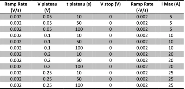
of the use of the system was possible outline a measurement plan taking into account the main current levels included in the domain of the transformer reached through five different current ramp rate (Table 4.1). The granularity with which the test runs were distributed was graded according to the different ramp rates: the current difference between consecutive measurements is short for lower ramp rate runs, while it is increased as the ramp rate increases.
Ramp Rate (A/s) 50 100 300 500 800 Current step (A) 500 500, 1000, 1500 500, 1000, 1500 1000, 1500 1500, 2000 Current Range (A) From 500 to 20000 From 500 to 24500 From 500 to 24500 From 500 to 23000 From 500 to 30500
Table 4.5 Summary of the system identification measurements.
The considered current ramp rates start from a minimum of 50 A/s up to 800 A/s, the maxim current increasing steps are then selected from a minimum value of 500 A to a maximum of 2000 A in the last runs at 800 A/s. The current domain explored reaches a maximum value of 30500 A, achieved by an 800 A/s ramp rate. At this stage the collected data were subjected to a post-processing phase where the calculated offset was removed from the measures. The result was a set of one hundred twenty-five measurements run where for each test run were measured the input signal VRef, the current on the transformer primary IP and on
the secondary ISec. To derive a model from this data set several consecutive
working regions were recognized. In each region is identified by considering the range where the system could be approximated by the same continuous time transfer function. When a transfer function is not able anymore to map satisfactorily the system dynamics, a new region has begun. Twelve regions were identified (Fig. 4.2) throughout the operating range (i.e. from 0 to 36 000 A).
47
Figure 4.2 partitions of the operating domain.
It is worthy to note that the system dynamic, for each working condition was identified independently from the ramp rate; in particular the function defined for each region approximates the behaviour of the system for every considered ramp rate. At the end of this analysis to synthesize a single model of the entire system domain (Fig. 4.3), the various functions have been included into a Sugeno fuzzy system [1].
Figure 4.3 simulated system model.
The fuzzy system input variable is the power supplier input voltage VRef, the same
of system to be controlled. The domain of this variable was fuzzyfied by taking into account the operating regions identified looking at the secondary current