c
ESO 2019
Astrophysics
&
Multiphase quasar-driven outflows in PG 1114+445
I. Entrained ultra-fast outflows
Roberto Serafinelli
1,2,3, Francesco Tombesi
1,4,5,6, Fausto Vagnetti
1, Enrico Piconcelli
6,
Massimo Gaspari
7,?, and Francesco G. Saturni
6,81 Dipartimento di Fisica, Università di Roma “Tor Vergata”, Via della Ricerca Scientifica 1, 00133 Roma, Italy
e-mail: [email protected]
2 Dipartimento di Fisica, “Sapienza” Università di Roma, Piazzale Aldo Moro 5, 00185 Roma, Italy 3 INAF – Osservatorio Astronomico di Brera, Via Brera 28, 20121 Milano, Italy
4 X-ray Astrophysics Laboratory, NASA/Goddard Space Flight Center, Greenbelt, MD 20771, USA 5 Department of Astronomy, University of Maryland, College Park, MD 20742, USA
6 INAF – Osservatorio Astronomico di Roma, Via Frascati 33, 00044 Monte Porzio Catone, Roma, Italy 7 Department of Astrophysical Sciences, Princeton University, 4 Ivy Lane, Princeton, NJ 08544-1001, USA 8 Space Science Data Center, Agenzia Spaziale Italiana, Via del Politecnico snc, 00133 Roma, Italy
Received 14 February 2019/ Accepted 5 June 2019
ABSTRACT
Substantial evidence in the last few decades suggests that outflows from supermassive black holes (SMBH) may play a significant role in the evolution of galaxies. These outflows, powered by active galactic nuclei (AGN), are thought to be the fundamental mechanism by which the SMBH transfers a significant fraction of its accretion energy to the surrounding environment. Large-scale outflows known as warm absorbers (WA) and fast disk winds known as ultra-fast outflows (UFO) are commonly found in the spectra of many Seyfert galaxies and quasars, and a correlation has been suggested between them. Recent detections of low ionization and low column density outflows, but with a high velocity comparable to UFOs, challenge such initial possible correlations. Observations of UFOs in AGN indicate that their energetics may be enough to have an impact on the interstellar medium (ISM). However, observational evidence of the interaction between the inner high-ionization outflow and the ISM is still missing. We present here the spectral analysis of 12 XMM-Newton/EPIC archival observations of the quasar PG 1114+445, aimed at studying the complex outflowing nature of its absorbers. Our analysis revealed the presence of three absorbing structures. We find a WA with velocity v ∼ 530 km s−1,
ionization log ξ/erg cm s−1∼ 0.35, and column density log N
H/cm−2∼ 22, and a UFO with vout ∼ 0.145c, log ξ/erg cm s−1∼ 4, and
log NH/cm−2∼ 23. We also find an additional absorber in the soft X-rays (E < 2 keV) with velocity comparable to that of the UFO
(vout∼ 0.120c), but ionization (log ξ/erg cm s−1∼ 0.5) and column density (log NH/cm−2∼ 21.5) comparable with those of the WA.
The ionization, velocity, and variability of the three absorbers indicate an origin in a multiphase and multiscale outflow, consistent with entrainment of the clumpy ISM by an inner UFO moving at ∼15% the speed of light, producing an entrained ultra-fast outflow (E-UFO).
Key words. X-rays: galaxies – quasars: general – quasars: individual: PG 1114+445 – galaxies: active
1. Introduction
Supermassive black holes (SMBH) in active galactic nuclei (AGN) are thought to be fundamental players in the evolution of their host galaxies. This is evident since host-galaxy properties, such as the stellar velocity dispersion (e.g.,Ferrarese & Merritt 2000) and the mass of the bulge (e.g.,Häring & Rix 2004), are correlated with the black hole mass. This suggests the exis-tence of a “feedback” mechanism between AGN activity and the star formation process, and disk winds are the most promising candidates to drive such processes (e.g., King & Pounds 2015; Fiore et al. 2017).
Moderately ionized winds (ξ . 100 erg cm s−1) are often detected in the soft X-ray band as blue-shifted absorption lines and edges, indicating that these so-called warm absorbers (WA) have velocities in the range v ∼ 100−1000 km s−1(e.g.,Halpern 1984;Blustin et al. 2005;Kaastra et al. 2014). Another class of winds, detected through X-ray absorption in AGNs, known as
? Lyman Spitzer Jr.Fellow.
ultra-fast outflows (UFOs), is characterized by a much higher ionization state (ξ ∼ 103−106erg cm s−1) and velocity (v ∼ 0.1 − 0.4c), measured through absorption lines of highly ionized gas, most often FeXXVand FeXXVI(e.g.,Chartas et al. 2002; Pounds et al. 2003a,b;Tombesi et al. 2010a,b,2011,2014,2015; Giustini et al. 2011; Gofford et al. 2013; Nardini et al. 2015; Vignali et al. 2015;Braito et al. 2018).
Tombesi et al. (2013) found that WA and UFO parameters show overall trends in a sample of 35 Seyfert galaxies and quasars. This may suggest that WAs and UFOs could be different phases of a large-scale outflow. In particular, UFOs are launched at relativis-tic velocities, probably from the inner parts of the accretion disk surrounding the central SMBH, while WAs are most likely located at larger distances. However, there have been recent detections of fast outflows also in the soft X-ray band (e.g.,Gupta et al. 2013, 2015; Longinotti et al. 2015; Pounds et al. 2016; Reeves et al. 2016), with identification of highly blue-shifted Kα lines of OVI
and OVII, suggesting high velocity (v ∼ 0.1−0.2c), but lower ion-ization states than typical UFOs.
UFOs are thought to have a significant impact on the inter-stellar medium (ISM) of their host galaxy. In fact, current models (e.g.,King 2003,2005) predict that inner UFOs may shock the ISM, transferring their kinetic energy to the ambient medium and possibly driving feedback on their host galaxy. In the aftermath of the shock, such models predict four regions being formed: (i) the inner UFO, (ii) the shocked UFO, (iii) the shocked swept-up ISM, and (iv) the outer ambient medium, not yet affected by the inner outflows. If the hot shocked gas cools down e ffec-tively, which means that the cooling time is shorter than the flow time, only momentum is conserved. In the opposite case of negligible cooling, the energy is conserved and hence the UFO transfers its kinetic power to the ISM (e.g., Costa et al. 2014; King & Pounds 2015), possibly clearing out the galaxy of its own gas (e.g.,Zubovas & King 2012). Even though direct evidence of the shocked ISM has been claimed in the past (Pounds & Vaughan 2011), it has been recently proposed that the observed low-ionization UFOs are due to shocked ISM by the inner UFO (Sanfrutos et al. 2018).
In addition, Gaspari & Sa¸dowski (2017) have shown that galaxy evolution might be regulated by a duty cycle between such multiphase AGN feedback, and a feeding phase that is thought to be due to so-called chaotic cold accretion (CCA; Gaspari et al. 2013), which is the cooling of gas clumps and clouds that “rain” toward the innermost regions of the AGN (e.g., Gaspari et al. 2018). While observational evidence of the feed-back phase has been extensively collected in the last two decades in many spectral rest-frame bands, such as X-rays, optical, UV, and sub-millimetric (see, e.g., Fiore et al. 2017; Cicone et al. 2018, for recent reviews), only recent observations are starting to detect the feeding phase (e.g., Tremblay et al. 2016, 2018; Lakhchaura et al. 2018;Temi et al. 2018).
PG 1114+445 is a type-1 quasar at z = 0.144 (Hewett & Wild 2010). The mass of the central SMBH and the bolometric luminosity are estimated (Shen et al. 2011) as log(M/M ) ∼ 8.8
and log(Lbol/erg s−1) ∼ 45.7, respectively, implying an
Edding-ton ratio of L/LEdd∼ 7%. The source was observed in 1996 by
the Advanced Satellite for Cosmology and Astrophysics (ASCA) in the X-ray band and by Hubble Space Telescope (HST) Faint Object Spectrograph (FOS) camera in the UV band. The X-ray analysis (George et al. 1997) showed the presence of an ionized WA in the soft band, interpreted as photoelectric absorption edges of OVIIand OVIII. Moreover, a detection of a possible absorp-tion line at E = 7.25+0.42−0.48keV was interpreted as being due to highly ionized iron, possibly suggesting the presence of a mildly relativistic outflow with v ∼ 0.1c. The investigation of the UV spectrum (Mathur et al. 1998) discovered CIVand Lyα narrow absorption lines (NAL), with line-of-sight velocities of vout ∼
530 km s−1. Given the similar ionization state of the soft X-ray and UV absorption features,Mathur et al.(1998) concluded that they are likely to originate from the same material.
In 2002, a much higher quality X-ray spectrum was obtained by a 44 ks XMM-Newton observation. These data revealed the complex two-component nature of the WA (Ashton et al. 2004; Piconcelli et al. 2005). In a recent ensemble work on a sam-ple of optically selected quasars in XMM-Newton archival data (Serafinelli et al. 2017), we used 11 additional archival spec-tra, also included in a recent study based on the two-corona model (Petrucci et al. 2018). Here we present a detailed spec-tral analysis of these data, together with a re-analysis of both the 2002 XMM-Newton and the 1996 ASCA observations, aimed at unveiling the multiphase nature of the outflows of PG 1114+445. The article is structured as follows. Section2describes the data reduction techniques used for these spectra. We show the
spectral analysis and results in Sect. 3. The distances of the absorbers are computed in Sect.4, while the energetics of the wind is described in Sect. 5. We summarize and discuss the results in Sect.6. Throughout the paper we have use the follow-ing cosmology: H0= 70 km s−1Mpc−1,Ωm= 0.3 and ΩΛ= 0.7.
2. Observations and data reduction
XMM-Newton observed PG 1114+445 on twelve occasions between 2002 and 2010. In May 2002 it was observed for ∼44 ks (OBSID 0109080801). Then, a campaign of 11 observations was performed between 2010 May 19 and 2010 December 12 (sequential OBSIDs from 0651330101 to 0651331101), for a total duration of ∼380 ks. Details on duration and exposure of the single observations are given in Table A.1. We extracted the event lists of the European Photon Imaging Camera (EPIC) detectors, both pn and Metal Oxide Semi-conductor (MOS), with the standard System Analysis Software (SAS, version 16.0.0) tools epproc and emproc. All observations are affected by background particle flaring (e.g.,De Luca & Molendi 2004; Marelli et al. 2017) to different extents, particularly OBSIDs from 0651330201 to 0651330501 (see Table A.1 for details). Therefore, we applied an appropriate filtering to remove the times affected by this effect. After checking that no pile-up (e.g.,Ballet 1999) correction was needed for any of these obser-vations, we extracted the spectra by selecting a region in the CCD image of 4000 radius around the source, and the back-ground by extracting a source-free region of the same size. We generated response matrices and auxiliary response files using the SAS tools rmfgen and arfgen respectively. Finally, we grouped the spectra by allowing 50 counts for each spectral bin using specgroup, considering a minimum energy width of one fifth of the full width half-maximum (FWHM) resolu-tion. XMM-Newton MOS1 and MOS2 spectra were combined to obtain a higher signal-to-noise ratio (S/N). We considered the 0.3−10 keV band of each spectrum.
We reduced the Reflection Grating Spectrometer (RGS) spectra by using rgsproc, screening times with high particle background through the examination of the RGS light curves, and using rgsfilter and rgsspectrum to produce clean spec-tra. However, we could not perform a statistically meaningful analysis because, even combining all 24 RGS1 and RGS2 spec-tra together with rgscombine, we obtained a combined mean spectrum with insufficient S/N. We also analyzed the 150 ks 1996 ASCA observation (ID 74072001), for which we retrieved
the already reduced data products from the Tartarus ASCA AGN database (Turner et al. 2001).
For simplicity, we gave each observation a simple identifi-cation code, where Obs. A represents the ASCA observation, Obs. 0 is the 2002 XMM-Newton observation, while Obs. 1 to Obs. 11 label the 2010 campaign observations (see TableA.1). Finally, we grouped together Obs. 1–3, 4–5, and 8–9 in order to increase the count rates of the single observations, mostly due to severe background particle screening, in order to reach a level of S/N adequate for the spectral analysis.
3. Spectral analysis
3.1. Models
The X-ray spectral analysis was carried out using the soft-ware XSPEC (Arnaud 1996) included in the High-Energy
1 https://heasarc.gsfc.nasa.gov/FTP/asca/data/
10−5 10−4 10−3 n o rm a liz e d c o u n ts s − 1 k e V − 1 c m − 2 1 0.5 2 5 0.5 1 1.5 2 ra ti o Energy (keV) 10−5 10−4 10−3 n o rm a liz e d c o u n ts s − 1 k e V − 1 c m − 2 1 0.5 2 5 1 1.5 ra ti o Energy (keV) 10−5 10−4 10−3 n o rm a liz e d c o u n ts s − 1 k e V − 1 c m − 2 1 0.5 2 5 1 1.5 ra ti o Energy (keV)
Fig. 1. Spectral fits of EPIC-pn and EPIC-MOS1+2 data of Obs. 0.
When only a continuum and blackbody model is included, the model poorly fits the data (top). We added an absorber, obtaining a significant improvement in the fit quality (middle). Our best fit model is obtained by adding a second absorber to the model (bottom).
Astrophysics SOFTware (HEASOFT) v6.18 software package. We fitted separately EPIC-pn and EPIC MOS1+2 spectra for each XMM-Newton observation, using a power law model with Galactic absorption, a soft excess modeled by a blackbody spec-trum, and two ionized absorbers (named Absorber (Abs.) 1 and Abs. 2), following indications from previous analyses of these spectra (Ashton et al. 2004;Piconcelli et al. 2005).
The best fit values of EPIC-pn and MOS spectra agree within a 90% confidence level (see Figs.C.1 andC.2), there-fore the results were recomputed fitting EPIC-pn and MOS spectra together, to obtain higher significance results. For the ASCA observation, we fitted together the spectra from all cam-eras of the telescope. Best-fit parameters of each spectra and the improvements in term of∆χ2for each fit component are listed
in TablesB.1–B.4, while spectra and best-fit curves are shown in Figs.D.1–D.8. In Fig.1, we show the spectra and ratio of the continuum, continuum+Abs. 1, and continuum+Abs. 1+Abs. 2 models for Obs. 0.
We rule out instrumental artifacts or random fluctuations for the detection of Abs. 2 for the following reasons. First, the main spectral features are detected in the observed energy range E = 0.8−1.5 keV, where no sharp edges are present in the effec-tive area of both pn and MOS instruments. Second, if due to an instrumental artifact, the spectral features would have been detected at the same energy and with the same intensity in many other sources. Third, in case of instrumental artifact, we would not observe the same features in both pn and MOS within a 90% confidence level for all the observations.
For three XMM-Newton observations, Obs. 1+2+3, Obs. 6, and Obs. 8+9, we also need a third absorber (Abs. 3) in the Fe Kα band, associated with a UFO. In TableB.3 we also report the best fit results for a third absorber in the ASCA observa-tion, although it is found with significance below a 2σ confi-dence level threshold, in order to compare with the claim of George et al.(1997). We note that the detection probability of all the UFO reported in TableB.3is higher than 99%, even when considering a blind line search. In fact, extensive Monte Carlo simulations show that the null probability of a spectral feature in the E= 7−10 keV band, with ∆d.o.f. = 3 (degrees of freedom), is ∼1% for a∆χ2& 11 (Tombesi et al. 2010a).
We modeled the ionized absorbers by computing detailed grids with the photoionization codeXSTAR(Kallman & Bautista 2001), which considers absorption lines and edges for every element with Z ≤ 30. For Abs. 1 and 2, we calculated an
XSTAR table with a spectral energy distribution in the E = 10−1−106eV energy band described by a photon index of
Γ = 2, with cutoff energy beyond Ec > 100 keV,
follow-ing Haardt & Maraschi (1991). We considered standard solar abundances from Asplund et al. (2009) and turbulent velocity of 100 km s−1 (e.g.,Laha et al. 2014). This value is well within
the energy resolution provided by the EPIC-pn and MOS instru-ments, and testing different values did not provide statistically different results. Since Abs. 3 is associated with UFOs, we adopted a nearly identical model, with the only difference being a larger turbulent velocity, v ∼ 103km s−1.
In the XSTAR grids, the free parameters are the absorber column density, NH, its observed redshift, zo, and the
ioniza-tion parameter, ξ = Lion/r2n, where Lion is the ionizing
lumi-nosity between 13.6 eV and 13.6 keV, computed by using the luminosity task inXSPECon the unabsorbed best fit spectral model. The relation between the observed redshift zo, the
cosmo-logical redshift zc, and the Doppler shift zaof the absorber with
respect to the source rest frame is 1+ zo = (1 + za)(1+ zc).
The velocity of the outflow is related to zaby the relation
1+ za=
s 1 − v/c 1+ v/c.
In case of outflowing material, zais a blueshift, and we
7×10²¹ 7.5×10²¹ 8×10²¹ 8.5×10²¹ 1 .5 × 1 0 2 1 2 × 1 0 2 1 NH ,2 ( c m − 2) NH,1 (cm −2) + 0.32 0.34 0.36 0.38 0.4 0 .5 1 lo g ξ2 ( e rg c m s − 1) logξ1 (erg cm s−1) +
Fig. 2.Contour plots of column density (left) and ionization parameter (right) of Abs. 1 vs. Abs. 2 for Obs. 0. Red, green, and blue lines represent
68%, 90%, and 95% confidence levels, respectively. The black cross represents the best-fit values.
0.5 1 − 0 .0 5 0 0 .0 5 z2 logξ2 (erg cm s−1) +
Fig. 3. Contour plot of the observed redshift of Abs. 2, i.e. zo,2, vs.
the ionization log ξ2 for Obs. 0. Red, green, and blue lines represent
68%, 90%, and 95% confidence levels, respectively. The black cross represents the best-fit values.
3.2. Results
Absorber 1 shows a very low variability (see TableB.1) in both ionization parameter log(ξ1/erg cm s−1) = 0.35 ± 0.04 and
col-umn density log(NH,1/cm−2) = 21.88 ± 0.05. The redshift of
the absorber, mainly due to the shift of the Fe M-shell unre-solved transition array (UTA), is comparable with the cosmo-logical one of the source (zo = zc) within the EPIC energy
resolution. In fact, when the absorber redshift is left free, the difference between the source redshift and the observed one is on the order of∆z ∼ 10−3, far below the energy resolution of
the instrument. Therefore, its velocity is assumed to be fixed at v1,out ∼ 530 km s−1, as shown by its corresponding
absorp-tion phase in the UV band (Mathur et al. 1998). These values of column density, velocity, and ionization are typical of a WA (Blustin et al. 2005).
Absorber 2 is more variable, as shown in Table B.2, with median values for the ionization parameter and column density given by log(ξ2/erg cm s−1)= 0.50 ± 0.36 and log(NH,2/cm−2)=
21.5 ± 0.2, respectively. We verified that the values of the
Table 1. Median values and median absolute deviation (MAD) for each parameter of three absorbers using the best-fit values of the XMM-Newtonspectra.
Parameter Median Units
log NH,1 21.88 ± 0.05 cm−2 log ξ1 0.35 ± 0.04 erg cm s−1 v1,out(∗) ∼530 km s−1 log NH,2 21.5 ± 0.2 cm−2 log ξ2 0.50 ± 0.36 erg cm s−1 v2,out 0.120 ± 0.029 c log NH,3(∗∗) 22.9 ± 0.3 cm−2 log ξ3 4.04 ± 0.29 erg cm s−1 v3,out 0.145 ± 0.035 c
log Lion 45.4 ± 0.3 erg s−1
Notes. We also report the median ionizing luminosity Lion. They were
computed putting together lower and upper limits of each parameter of the XMM-Newton observations. Units are reported; in the case of loga-rithmic parameters, the units are to be understood as related to the argu-ment.(∗)The value of v
1,outwas set to 530 km s−1, followingMathur et al.
(1998).(∗∗)We computed median and MAD for the lower values of N H,3,
since we only have lower limits for two observations (see TableB.3).
parameters of Abs. 2 are independent from the ones of Abs. 1, ruling out any systematically induced correlation. In fact, even if the median values of the two absorbers are of the same order, the values of the individual observations are not correlated. Indeed, the correlation coefficient between non-fixed values of NH,1and
the corresponding NH,2 is r = 0.14, while the one between
log ξ1 and log ξ2 is r = 0.17, showing that their variability is
not related. Moreover, contour plots show no significant corre-lation between the column density and ionization parameter of Abs. 1 and Abs. 2 (see Fig. 2). The velocity of this absorber is measured with respect to the centroid energy of UTA Fe M and oxygen lines for the observations with lower ionization parameter, and the addition of Fe L lines for the observations with higher ionization parameter, such as Obs. 7 and 11 (see TableB.2). Given the low resolution of the EPIC cameras, how-ever, only Fe UTA are likely to contribute to the redshift calcu-lation. As shown in Fig. 3, contour plots of the observed red-shift zo,2and log ξ2are well constrained. However, the observed
Fig. 4. Time dependence of the out-flow velocity vout(top), ionization
param-eter ξ (middle), and column density NH
(bottom). For each panel we show the val-ues of Abs. 1 (red stars), Abs. 2 (green tri-angles), and Abs. 3 (blue squares). Lower limits on NHwere marked with an arrow.
Horizontal lines with shaded bands rep-resent the median values and the corre-sponding median absolute deviations.
redshift is below the systemic value zc= 0.144 even at 95%
con-fidence level. The median value of the velocity of this absorber is v2,out= (0.120 ± 0.029)c. Given the high velocity and low values
of the ionization and column density, this absorber shows inter-mediate parameters between a WA and a UFO. In fact, outflows with v ∼ 0.1−0.4c are usually coupled with ionization parame-ters in the range log ξ/erg cm s−1 ∼ 3−6 (Tombesi et al. 2013), detectable by observing Fe XXV and XXVI absorption lines. The ionization parameter of this absorber is instead in the range log ξ2/erg cm s−1∼ 0−1.5, much lower than the usual UFO and
comparable with the range of ionization we find in WAs. As mentioned, three observations show evidence of a third absorber. This absorber is variable (see Table B.3) and the median values of column density, ionization, and velocity are respectively log(NH,3/cm−2) = 22.9 ± 0.3, log(ξ3/erg cm s−1)=
4.04 ± 0.29, and v3,out= (0.140 ± 0.035)c. These values are
con-sistent with those of a typical UFO (e.g., Tombesi et al. 2011; King & Pounds 2015). The median values of all the parameters of the three absorbers are summarized in Table1, while the best-fit results of each absorber in time are shown in Fig.4.
While the WA and the UFO agree with the linear trends in Tombesi et al. (2013) between column density, ionization parameter, and velocity, Abs. 2 does not fit well into such rela-tions (see Figs.5–7) and it lies in a different region of the plots. It is straightforward to note that the velocity of Abs. 2 and that of the UFO are consistent within their dispersion, while ξ and NHare consistent with those of the WA. This is a strong
indi-cation that this absorber is likely to be an intermediate phase between these two, possibly related to the interstellar medium
being entrained by the UFO (see Sect.5), and hence we can name this absorber the entrained ultra-fast outflow (E-UFO).
4. Distances of the absorbers
Following Tombesi et al. (2013) and Crenshaw & Kraemer (2012) we can estimate the maximum distance of the absorber from the black hole, by assuming that the shell size is smaller than its distance from the center, meaning NH = nR < nr,
with R size of the shell and r distance from the SMBH, so that n = NH/rmax. The determination of a well-defined ionization
parameter indicates that we are observing a shell of gas with a thickness much smaller than the average distance of the absorber to the source, otherwise we would have detected a significantly larger gradient in the ionization parameter. Therefore we have rmax=
Lion
NHξ
, (1)
where Lionis the unabsorbed ionizing luminosity emitted by the
source, for which we used the median value reported in Table1. We are also able to compute the minimum distance from the black hole, by computing the distance at which the observed velocity is equal to the escape velocity,
rmin=
2GMBH
v2out · (2)
For the warm absorber, we obtain rmin,WA ∼ 105rs ' 18 pc
Fig. 5.Velocity vs. ionization parameter plot for warm absorber (red stars), entrained ultra-fast outflow (green triangles), and ultra-fast out-flow (blue squares). As expected, the UFO and the WA seem to follow a linear correlation. The smaller black points and the dashed line repre-sent the points and the linear fit ofTombesi et al.(2013). The velocity of the WA constant to the value computed byMathur et al.(1998) is v ∼ 530 km s−1. The E-UFO does not follow such a correlation. The
magenta points represent other soft X-ray UFOs reported in the litera-ture (see Sect.1for details).
Schwarzschild radius. Since no constraints can be put on these values, we have to assume that the WA is located beyond rmin,WA.
However, the external radius rmax,WAis too extreme and therefore
we do not report it on Table2. We assume instead a typical value rmax,WA∼ 3 kpc (Di Gesu et al. 2013).
For the UFO, we obtain rmin,UFO∼ 57rs' 3 × 10⁻³pc
and rmax,UFO∼ 104rs ' 0.5 pc. Numerical simulations (e.g., Fukumura et al. 2015;Nomura et al. 2016;Sa¸dowski & Gaspari 2017) show that the UFO launching region is confined within r . 100rs and therefore we conservatively assume rmin,UFO as
the typical value of the distance of the UFO from the central SMBH.
Having a UFO-like velocity, the minimum distance of the E-UFO from the central SMBH is much smaller than that of the WA, which is rmin,E-UFO∼ 70rs. However, this value that is
consistent with the distance of the UFO is not applicable, since a clumpy wind co-spatial with the UFO at r < 100rs (e.g., Pounds et al. 2016) is excluded on the basis of photoionization considerations. In fact, the absorber would require a Compton-thick column density in order to be shielded from the intense radiation field and at the same time preserve its low ionization parameter. Moreover, the consistent values of both NH and ξ
between the WA and the E-UFO strongly suggest that the two absorbers share the same material, hence they are at comparable distances from the SMBH. Therefore, the E-UFO is most likely located in a shell with rmin,E-UFO& 18 pc, in agreement with the
location of the WA.
An alternative method to compute the distance of the absorber from the SMBH is to use the median absolute devia-tions (MAD) of NH and vout to estimate a typical value of the
Fig. 6. Velocity vs. column density plot for WA (red stars), E-UFO
(green triangles), and UFO (blue squares). As in the case of Fig. 5, the warm absorber and the ultra-fast outflow are in agreement with
Tombesi et al.(2013) (smaller black dots and dashed line). Arrows
rep-resent lower limits on NH. Magenta points are soft X-ray UFOs in the
literature. Again, the velocity of the warm absorber is assumed to be v ∼530 km s−1. Even though the green triangles do not follow the linear
fit ofTombesi et al.(2013), there seems to be some continuity between the column density of this absorber and the “regular” ultra-fast outflows.
Fig. 7.Column density vs. ionization parameter plot for WA (red stars),
E-UFO (green triangles), and UFO (blue squares). Arrows represent lower limits on the column density, with the black dots and dashed line representing the linear fit fromTombesi et al.(2013). Magenta points are soft X-ray UFOs from the literature. This plot does not show any dif-ference fromTombesi et al.(2013), since the E-UFO only differs from
Table 2. Distance, density, mass outflow rate, momentum rate and kinetic power for each absorber.
r/rs r(pc) n(cm−3) M˙out(M yr−1) P˙out/ ˙Prad E˙K/Lbol
Warm absorber rmin,WA 3.2 × 10⁵ 18 3.6 × 10⁵ 2.63 Cv 0.05 Cv 4.2 × 10⁻⁵Cv rmax,WA 5.2 × 10⁷ 3 × 10³ 13 430 Cv 8 Cv 7 × 10⁻³Cv Entrained UFO rvar,E-UFO 1.7 × 10⁶ 110 7.5 × 10³ 400 Cv 495 Cv 29 Cv Ultra-fast outflow rmin,UFO 57 3.2 × 10⁻³ 2.3 × 10⁹ 0.41 0.62 0.04
Notes. The distance from the black hole r is given in both units of Schwarzschild radius rs= 2GMBH/c2and parsec. We listed the estimated density
nat such a distance, mass outflow rate in units of solar masses per year, momentum rate in units of the radiation momentum rate ˙Prad = Lbol/c,
and kinetic power in units of Lbol. The symbol Cvrepresents the filling factor of the region, assumed unitary for the region containing the UFO.
We use MBH ∼ 5.9 × 10⁸M and Lbol ∼ 5.5 × 1045erg s−1fromShen et al.(2011). For UFO and E-UFO we only reported the most likely value
for the distance of the absorber, while for the WA it is not possible to constrain the region, therefore we report the values computed using rmin, and
consider a typical value for the upper limit of rmax,WA∼ 3 kpc (Di Gesu et al. 2013).
density of the absorber. Since a significant degree of clumpiness is expected for the ambient medium (e.g.,Gaspari & Sa¸dowski 2017), it is reasonable to assume that the variations of the typical shell radius R are due to the velocity dispersion∆vout. However,
this is due to the fact that the shell’s apparent thickness depends on the peculiar clump we are observing, and it is not due to an intrinsic variability of the velocity and the physical properties of the gas in the clump.
To derive an estimate of the shell’s apparent thickness we consider NH' nR, and we can obtain through partial derivation
∆NH ∆t = n ∆R ∆t + R ∆n ∆t· (3)
We assume that in the time span of the XMM-Newton obser-vations,∆t ' 8.5 yr, the average density of the shell does not significantly vary, therefore ∆n/∆t ' 0, and we assume that ∆R/∆t corresponds to the MAD of the velocity of the absorber, ∆vout. Given the variability of NHand vout, we are able to
com-pute a typical value of the shell density and consequently the distance of the absorber from the black hole, using the following equations: hni= ∆NH ∆t∆vout , (4) rvar= s Lion hniξ· (5)
The distance of the E-UFO from the SMBH is therefore rvar,E-UFO∼ 2 × 10⁶rs' 109 pc, which is consistent with being at
least partially co-spatial with the WA at r& 18 pc.
However, these distance estimates are representative of the location of the three absorbers, but it is not physically required to define a division between the regions, given that there is unlikely to be a sharp physical discontinuity among them. All the values of the distance from the central black hole and density are sum-marized in Table2.
5. Outflow energetics
The mass outflow rate can be estimated following the equation inCrenshaw & Kraemer(2012),
˙
Mout = 4πµmpCvCfNHvoutr, (6)
where mp is the proton mass, while µ ≡ nH/ne ' 1/1.4 for
solar abundances. The symbol Cf represents the covering factor,
which we assume to be Cf ' 0.5 (e.g.,Tombesi et al. 2010a),
and Cv is the filling factor of the region, which we assume
to be unitary for the UFO, according to previous results (e.g., Nardini et al. 2015; Tombesi et al. 2015), and that we keep as parametric for both the E-UFO and WA. We also assume that E-UFO and WA also share the same clumpiness.
The momentum rate of the outflow is given by ˙
Pout = ˙Moutvout. (7)
Finally, we compute the kinetic power ˙ EK= 1 2M˙outv 2 out. (8)
We compute Eqs. (6)–(8) for each of the three absorbing complexes, using the median values of NHand vout(see Table1)
and the corresponding distance as computed in Sect.4. The com-plete set of r, ˙Mout, ˙Pout, and ˙EKvalues is listed in Table2, with
˙
Pout in units of the momentum rate of the AGN, ˙Prad = Lbol/c,
with Lbol = 5.5 × 1045erg s−1 (Shen et al. 2011), and ˙EK in
units of Lbol. The median velocities of E-UFO and UFO are
perfectly comparable within the errors. This suggests that these two absorbers are dynamically connected, which means that the two ionized absorbers have interacted. If we assume an energy-conserving interaction between the UFO and the E-UFO, the fill-ing factor of the region containfill-ing the entrained outflow must be Cv ' 1.4 × 10⁻³. However, we also obtain a very
simi-lar value assuming a momentum-conserving interaction between the UFO and the E-UFO. The density of the E-UFO region, as computed in Eq. (4), is hn2i ' 7.5 × 103cm−3. If we assume
for the UFO a distance from the black hole r3 ≥ rmin, we
obtain n3 ≤ Lion/ξrmin2 ' 2.3 × 109cm−3. Assuming a
mass-conserving spherical shell, the density scales as n ∝ r−2, and
the predicted value of the density at rvar ' 110 pc would be
n2 . 120 cm−3, around a factor of ∼100 lower than the one
obtained with variability arguments. This means that the aver-age density computed with Eq. (4) is dominated by the density of the clumps in the E-UFO region. Moreover, if we assume that NH∝ n, since NH,3' 5 × 1023cm−2, the UFO column density at
rvar would be NH ∼ 1016cm−2, much lower than the observed
NH,2 ' 3.1 × 1021cm−2, which supports our requirement for
Fig. 8. Diagram of the X-ray obser-vations of PG 1114+445. A UFO is present in the inner part of the AGN surroundings, with decreasing density, scaling as r−2. At larger distances from
the SMBH, the UFO interacts with the closest clumpy ambient gas at r ' 100 pc, entraining it via Rayleigh– Taylor and Kelvin–Helmholtz instabil-ities. This gas is pushed at veloci-ties comparable with that of the UFO, retaining its ionization state and col-umn density. The farther ambient gas remains unaffected by the UFO and therefore moves at a significantly lower line-of-sight velocity. The figure is not to scale.
of AGN feedback driven by outflows (Zubovas & Nayakshin 2014; Costa et al. 2014; Gaspari & Sa¸dowski 2017), in which Rayleigh–Taylor and Kelvin–Helmholtz instabilities, together with radiative cooling, cause the shell of shocked gas to frag-ment into clumpy warm and cold clouds that fill the nuclear and kiloparsec region. The clumpy environment and ensem-ble of cold or warm clouds is more in line with with the CCA scenario (Gaspari et al. 2013) instead of spherical hot-mode accretion (Bondi 1952). The typical core filling factor, obtained in simulations (Gaspari et al. 2017), is ∼0.1−1%, and supports our result. The mass outflow rate of the E-UFO is
˙
Mout,2 ' 0.55 M yr−1, which is ∼ 35% larger than the UFO
value ˙Mout,1 ' 0.41 M yr−1, possibly meaning that the mass is
growing by sweeping-up the material that is being entrained by the UFO.
Given that WA and E-UFO share the same gas properties (i.e., ionization and column density), we also assume that the two regions share the same filling factor, in which case we obtain
˙
Pout,1 ˙Pout,3 and ˙EK,1 ˙EK,3, which is compatible with the
fact that the two absorbers are not dynamically related, suggest-ing that the WA represents an unperturbed region that has not yet been significantly affected by the UFO.
6. Summary and discussion
We summarize our findings in graphical form by presenting the multiphase absorber of PG 1114+445 in the diagram shown in Fig. 8. Together with the analysis described in this work, such a scenario is also well supported by theoretical models of AGN outflow evolution (e.g.,King 2003,2005;Zubovas & King 2012), which predict an inner UFO driving into the surround-ing medium, sweepsurround-ing-up the gas outwards. In the aftermath of the shock, four regions are consequently formed: (i) the inner-most region, containing the unshocked UFO, (ii) the shocked inner wind, (iii) the shock-induced swept-up interstellar gas, and (iv) the unaffected ambient medium.
A UFO with high velocity (vout,3' 0.145c), ionization
param-eter, and column density (e.g.,Tombesi et al. 2011) is detected in three XMM-Newton observations. This absorber is located very close to the source, at r ∼ 3 × 10⁻³pc ' 60r
s(see Table2), and
can be associated with the inner wind, in agreement with detailed general-relativistic radiative magnetohydrodynamic (GR-rMHD) simulations (e.g., Sa¸dowski & Gaspari 2017). On the contrary, given its expected low particle density (see Sect.5), the shocked inner wind is likely to be undetectable with the present dataset,
since an expected column density of NH ∼ 1016cm−2is below
the sensitivity limit of current spectrometers.
The low values of v, log ξ, and NHfor the WA are
compat-ible with usual absorbers of this kind (e.g.,Blustin et al. 2005). Its low variability (see Fig.4) suggests that the WA is not dynam-ically connected to the inner UFO. In fact, WAs are believed to be relics of the original optically thick gas surrounding the black hole before any AGN activity started. This gas may have been driven towards larger distances by the initial radiation pressure of the quasar, until it became optically thin (King & Pounds 2014). Alternatively, the ambient clouds are drifting in the macro-scale turbulent velocity field (Gaspari & Sa¸dowski 2017), with velocities of a few hundred km s−1. Supported by the
con-stancy over more than a decade of observations, the WA is most likely part of the ambient medium, not yet significantly affected by the UFO.
A comparison between the v−ξ, v−NH and ξ−NHrelations
for the three absorbers (see Figs.5–7) shows that the WA and the UFO are well around the expected values (Tombesi et al. 2013), whereas, on the other hand, the E-UFO has the typical velocity of a UFO, but ionization and column density values comparable with the WA.
We interpret these three main absorbers phases as the time evolution of outflows that were expelled at different epochs from the SMBH accretion disk and are observed as the material is continuing to travel outwards. These considerations are valid under the plausible assumption that the mass accretion rate of the SMBH, and consequently the power of the UFO, did not signif-icantly change during a timescale of t ∼ r/v ∼ 100 pc/0.145c ∼ 2000 years, which is negligible compared to the minimum time required for the SMBH to double its mass, equal to the Salpeter time tS ∼ 5 × 10⁷yr. Moreover, we note that in
low-mass galaxy haloes, the AGN accretion duty cycle is almost quasi-continuous, thus allowing for the observation of multi-ple generations of AGN feedback events (Gaspari & Sa¸dowski 2017). Finally, the interaction between the UFO and the clumpy ambient medium is most likely Rayleigh-Taylor and Kelvin-Helmholtz unstable (e.g., King 2010; Zubovas & Nayakshin 2014;Costa et al. 2014), consistently with the variability of the E-UFO and its low volume filling factor Cv.
Our detection of three concurrent outflow phases in the same source provides a remarkable corroboration of the self-regulated mechanical AGN feedback scenario (e.g., King 2003, 2005; King & Pounds 2014;Gaspari & Sa¸dowski 2017). Similar con-clusions, however not considering a clumpiness of the ambient
medium, have been reached by Sanfrutos et al. (2018), for IRAS 17020+4544, in which all three phases have also been detected. The UFO, driven by the accreting SMBH, propagates to meso scales (parsec to kiloparsec), still with significant veloc-ity, where the entrainment and mixing with the turbulent and clumpy ambient medium becomes substantial (E-UFO). The outflow kinetic energy is then likely deposited at macro scales in the form of thermal energy, via bubbles, shocks, and turbu-lent mixing (Gaspari & Sa¸dowski 2017; Lau et al. 2017), thus re-heating the galaxy and the group gaseous halo. This self-regulated cycle may happen many times during the AGN’s life-time, giving rise to a symbiotic relation between the SMBH growth and the evolution of the host galaxy (Gaspari et al. 2017). The combination of multiepoch observations of nuclear winds and multiwavelength investigations of spectral fea-tures tracing multiphase parsec to kiloparsec outflows (e.g., Fiore et al. 2017) can be considered as the most promising strat-egy to shed light on the AGN feedback processes over a large range of distances from the central engine. In particular, UV and optical spectra of PG 1114+445 are currently being analyzed in order to link the physical properties of outflows in different spec-tral bands and will be the subject of upcoming articles.
Acknowledgements. We thank Valentina Braito, James Reeves, Cristian Vignali,
Jelle Kaastra, Andrew King, Andrew Lobban, and Riccardo Middei for discus-sions and suggestions. We thank the referee for useful suggestions that improved the quality of this article. RS, FV, and EP acknowledge financial contribution from the agreement ASI-INAF n.2017-14-H.0. FT acknowledges support by the Programma per Giovani Ricercatori – anno 2014 “Rita Levi Montalcini”. MG is supported by the Lyman Spitzer Jr. Fellowship (Princeton University) and by NASA Chandra grants GO7-18121X and GO8-19104X. The results are based on observations obtained with XMM-Newton, an ESA science mission with instru-ments and contributions directly funded by ESA Member States and NASA. This research has also made use of data and software provided by the High Energy Astrophysics Science Archive Research Center (HEASARC), which is a ser-vice of the Astrophysics Science Division at NASA/GSFC and the High Energy Astrophysics Division of the Smithsonian Astrophysical Observatory.
References
Arnaud, K. A. 1996, in Astronomical Data Analysis Software and Systems V,
eds. G. H. Jacoby, & J. Barnes,ASP Conf. Ser., 101, 17
Ashton, C. E., Page, M. J., Blustin, A. J., et al. 2004,MNRAS, 355, 73
Asplund, M., Grevesse, N., Sauval, A. J., & Scott, P. 2009, ARA&A, 47,
481
Ballet, J. 1999,A&AS, 135, 371
Blustin, A. J., Page, M. J., Fuerst, S. V., Branduardi-Raymont, G., & Ashton, C.
E. 2005,A&A, 431, 111
Bondi, H. 1952,MNRAS, 112, 195
Braito, V., Reeves, J. N., Matzeu, G. A., et al. 2018,MNRAS, 479, 3592
Chartas, G., Brandt, W. N., Gallagher, S. C., & Garmire, G. P. 2002,ApJ, 579,
169
Cicone, C., Brusa, M., Ramos Almeida, C., et al. 2018,Nat. Astron., 2, 176
Costa, T., Sijacki, D., & Haehnelt, M. G. 2014,MNRAS, 444, 2355
Crenshaw, D. M., & Kraemer, S. B. 2012,ApJ, 753, 75
De Luca, A., & Molendi, S. 2004,A&A, 419, 837
Di Gesu, L., Costantini, E., Arav, N., et al. 2013,A&A, 556, A94
Ferrarese, L., & Merritt, D. 2000,ApJ, 539, L9
Fiore, F., Feruglio, C., Shankar, F., et al. 2017,A&A, 601, A143
Fukumura, K., Tombesi, F., Kazanas, D., et al. 2015,ApJ, 805, 17
Gaspari, M., & Sa¸dowski, A. 2017,ApJ, 837, 149
Gaspari, M., Ruszkowski, M., & Oh, S. P. 2013,MNRAS, 432, 3401
Gaspari, M., Temi, P., & Brighenti, F. 2017,MNRAS, 466, 677
Gaspari, M., McDonald, M., Hamer, S. L., et al. 2018,ApJ, 854, 167
George, I. M., Nandra, K., Laor, A., et al. 1997,ApJ, 491, 508
Giustini, M., Cappi, M., Chartas, G., et al. 2011,A&A, 536, A49
Gofford, J., Reeves, J. N., Tombesi, F., et al. 2013,MNRAS, 430, 60
Gupta, A., Mathur, S., Krongold, Y., & Nicastro, F. 2013,ApJ, 772, 66
Gupta, A., Mathur, S., & Krongold, Y. 2015,ApJ, 798, 4
Haardt, F., & Maraschi, L. 1991,ApJ, 380, L51
Halpern, J. P. 1984,ApJ, 281, 90
Häring, N., & Rix, H.-W. 2004,ApJ, 604, L89
Hewett, P. C., & Wild, V. 2010,MNRAS, 405, 2302
Kaastra, J. S., Kriss, G. A., Cappi, M., et al. 2014,Science, 345, 64
Kallman, T., & Bautista, M. 2001,ApJS, 133, 221
King, A. 2003,ApJ, 596, L27
King, A. 2005,ApJ, 635, L121
King, A. R. 2010,MNRAS, 408, L95
King, A. R., & Pounds, K. A. 2014,MNRAS, 437, L81
King, A., & Pounds, K. 2015,ARA&A, 53, 115
Laha, S., Guainazzi, M., Dewangan, G. C., Chakravorty, S., & Kembhavi, A. K.
2014,MNRAS, 441, 2613
Lakhchaura, K., Werner, N., Sun, M., et al. 2018,MNRAS, 481, 4472
Lau, E. T., Gaspari, M., Nagai, D., & Coppi, P. 2017,ApJ, 849, 54
Longinotti, A. L., Krongold, Y., Guainazzi, M., et al. 2015,ApJ, 813, L39
Marelli, M., Salvetti, D., Gastaldello, F., et al. 2017,Exp. Astron., 44, 297
Mathur, S., Wilkes, B., & Elvis, M. 1998,ApJ, 503, L23
Nardini, E., Reeves, J. N., Gofford, J., et al. 2015,Science, 347, 860
Nomura, M., Ohsuga, K., Takahashi, H. R., Wada, K., & Yoshida, T. 2016,PASJ,
68, 16
Petrucci, P.-O., Ursini, F., De Rosa, A., et al. 2018,A&A, 611, A59
Piconcelli, E., Jimenez-Bailón, E., Guainazzi, M., et al. 2005,A&A, 432, 15
Pounds, K. A., & Vaughan, S. 2011,MNRAS, 413, 1251
Pounds, K. A., King, A. R., Page, K. L., & O’Brien, P. T. 2003a,MNRAS, 346,
1025
Pounds, K. A., Reeves, J. N., King, A. R., et al. 2003b,MNRAS, 345, 705
Pounds, K. A., Lobban, A., Reeves, J. N., Vaughan, S., & Costa, M. 2016,
MNRAS, 459, 4389
Reeves, J. N., Braito, V., Nardini, E., et al. 2016,ApJ, 824, 20
Sanfrutos, M., Longinotti, A. L., Krongold, Y., Guainazzi, M., & Panessa, F.
2018,ApJ, 868, 111
Sa¸dowski, A., & Gaspari, M. 2017,MNRAS, 468, 1398
Serafinelli, R., Vagnetti, F., & Middei, R. 2017,A&A, 600, A101
Shen, Y., Richards, G. T., Strauss, M. A., et al. 2011,APJS, 194, 45
Temi, P., Amblard, A., Gitti, M., et al. 2018,ApJ, 858, 17
Tombesi, F., Cappi, M., Reeves, J. N., et al. 2010a,A&A, 521, A57
Tombesi, F., Sambruna, R. M., Reeves, J. N., et al. 2010b,ApJ, 719, 700
Tombesi, F., Cappi, M., Reeves, J. N., et al. 2011,ApJ, 742, 44
Tombesi, F., Cappi, M., Reeves, J. N., et al. 2013,MNRAS, 430, 1102
Tombesi, F., Tazaki, F., Mushotzky, R. F., et al. 2014,MNRAS, 443, 2154
Tombesi, F., Meléndez, M., Veilleux, S., et al. 2015,Nature, 519, 436
Tremblay, G. R., Oonk, J. B. R., Combes, F., et al. 2016,Nature, 534, 218
Tremblay, G. R., Combes, F., Oonk, J. B. R., et al. 2018,ApJ, 865, 13
Turner, T. J., Nandra, K., Turcan, D., & George, I. M. 2001,AIP Conf. Proc.,
599, 991
Vignali, C., Iwasawa, K., Comastri, A., et al. 2015,A&A, 583, A141
Zubovas, K., & King, A. 2012,ApJ, 745, L34
Appendix A: Data
Table A.1. Data considered in this work for PG 1114+445.
ID OBSID Start date Instrument Exposure time (s) Counts (0.3–10 keV) A 74072000 1996-05-05 23:59:48 ASCA sis0+1 121 230 6089(∗) ASCA gis2+3 136 800 6138(∗) 0 0109080801 2002-05-14 15:27:00 EPIC-pn 32 500 23 462 MOS1+2 80 380 17 700 1 0651330101 2010-05-19 09:48:59 EPIC-pn 20 550 7166 MOS1+2 57 270 6418 2 0651330201 2010-05-21 09:41:13 EPIC-pn 9824 3924 MOS1+2 27 400 3213 3 0651330301 2010-05-23 10:06:23 EPIC-pn 5271 1669 MOS1+2 18 357 1792 4 0651330401 2010-06-10 07:28:14 EPIC-pn 10 740 5341 MOS1+2 32 750 5214 5 0651330501 2010-06-14 07:56:46 EPIC-pn 6613 2956 MOS1+2 16 804 2314 6 0651330601 2010-11-08 23:22:49 EPIC-pn 18 500 17 359 MOS1+2 46 400 12 704 7 0651330701 2010-11-16 22:50:52 EPIC-pn 16 240 9732 MOS1+2 46 510 9046 8 0651330801 2010-11-18 22:42:54 EPIC-pn 20 350 9707 MOS1+2 57 020 8490 9 0651330901 2010-11-20 22:35:32 EPIC-pn 21 350 12 244 MOS1+2 52 210 9724 10 0651331001 2010-11-26 23:40:17 EPIC-pn 17 660 8704 MOS1+2 46 040 7173 11 0651331101 2010-12-12 22:31:31 EPIC-pn 13 710 7439 MOS1+2 26 650 4562
Notes. In all the spectra, a binning of a minimum of 50 counts per bin has been used, with the only exception of the ASCA observation, for which the data were already reduced. A simplified identification code (ID) was assigned to each observation. Observations 2, 3, 4, and 5 are affected by high soft proton flaring background (e.g.,De Luca & Molendi 2004;Marelli et al. 2017). Such high background, especially for Obs. 3, is responsible for the low number of counts for these observations, resulting in the high errors of the fit results of these observations. For this reason, we merged the spectra of Obs. 1, 2, and 3, Obs. 4 and 5, and Obs. 8 and 9. The MOS exposure times and counts are intended to be the sum of such quantities for each camera.(∗)ASCA counts are computed in the 0.5−10 keV band.
Appendix B: Tables of best-fit results
Table B.1. Parameters of Abs. 1.
ID NH,1/1021cm−2 log(ξ1/erg cm s−1) ∆χ2 A 7.5(∗) 0.35(∗) 275 0 7.7+0.3−0.4 0.34+0.01−0.01 1990 1+2+3 7.5(∗) 0.35(∗) 1377 4+5 6.9+0.7−3.1 ≤0.32 1117 6 7.5+0.6−0.5 0.35+0.04−0.02 1852 7 7.9+0.5−0.3 0.33+0.01−0.01 1073 8+9 7.4+0.5−0.5 0.34+0.02−0.01 2182 10 7.6+0.6−1.0 0.37+0.06−0.03 880 11 7.5(∗) 0.35(∗) 648
Notes. We only show column density NH and ionization parameter log ξ, since the velocity is not resolvable by the current X-ray dataset. We
also show the significance of the absorber,∆χ2, with respect to the model with no absorbers, with∆d.o.f. = 2 . All the null probabilities P nullare
less than 10−12and therefore are not reported.(∗)For these observations, the two soft X-ray absorbers are not resolved, and therefore we fixed the
Table B.2. Parameters of Abs. 2.
ID NH,2/1021cm−2 log(ξ2/erg cm s−1) zo,2/10−2 v2/c ∆χ2 Pnull
A 7.8+0.6−1.4 0.34+0.63−0.06 +3.3+3.9−2.4 0.102+0.023−0.037 46 10−12 0 1.8+0.2−0.1 0.65+0.10−0.04 +1.7+1.4−1.3 0.117+0.013−0.012 68.4 10−11 1+2+3 3.7+0.1−0.1 0.26+0.05−0.03 −3.9+1.2−1.8 0.172+0.012−0.018 18.1 10−3 4+5 7.7+0.3−0.2 0.38+0.01−0.01 +6.4+1.5−1.4 0.073+0.014−0.013 20.4 3 × 10⁻⁴ 6 2.7+0.2−0.2 0.06+0.02−0.02 −2.1+1.2−1.4 0.155+0.012−0.014 61 3 × 10⁻¹¹ 7 6.7+0.9−1.0 1.39+0.07−0.10 +6.4+1.3−1.6 0.073+0.012−0.015 26.0 6 × 10⁻⁶ 8+9 3.0+0.2−0.1 0.63+0.06−0.03 +1.1+1.0−0.8 0.123+0.010−0.008 73.4 4 × 10⁻¹⁵ 10 3.0+0.2−0.2 0.35+0.04−0.05 +1.4+1.2−1.6 0.132+0.012−0.016 32.1 10−6 11 5.4+0.7−0.6 1.22+0.07−0.08 +3.6+1.0−2.0 0.100+0.009−0.019 78 3 × 10⁻¹²
Notes. The column density NH, ionization parameter log ξ, and observed redshift of the absorber zo. The velocity of the absorber, in units of v/c,
with c the speed of light, is also shown. We report the significance of this absorber,∆χ2, with∆d.o.f. = 3, and the null probability P
nullrelated to
the model with one absorber.
Table B.3. Parameters of Abs. 3.
ID NH,3/1021cm−2 log(ξ3/erg cm s−1) zo,3/10−2 v3/c ∆χ22abs Pnull,2abs ∆χ21abs Pnull,1abs
A ≥ 440 3.83+0.21−0.21 +0.2+0.5−0.5 0.132+0.005−0.005 / / / /
1+2+3 143+606−69 3.85+0.47−0.14 +5.9−0.9+0.5 0.078+0.005−0.008 20.0 4 × 10⁻⁴ 21.1 3 × 10⁻⁴ 6 ≥ 295 4.43+0.22−0.34 −1.2+0.5−0.4 0.145+0.005−0.004 11.8 0.01 13.5 0.01 8+9 75+125−36 3.77+0.23−0.13 −4.7+0.5−0.7 0.173+0.005−0.007 12.0 7 × 10⁻³ 12.4 0.01
Notes. Again, column density NH, ionization parameter log ξ, and the observed redshift zoare shown. For the ASCA observation and XMM-Newton
Obs. 6, we are only able to report a lower limit for the column density. The velocity of this absorber is also reported in units of v/c. We show the significance of this absorber,∆χ2
2abs, with∆d.o.f. = 3, and the null probability Pnull,2abs, with respect to the model with two absorbers. Moreover,
the same quantities with respect to the model with only Abs. 1, i.e.∆χ2
1absand Pnull,1abs, are also shown. The UFO in the ASCA observation is not
detected above a threshold confidence level of 2σ. However, we report the best-fit result, in agreement with the previous claim byGeorge et al.
(1997).
Table B.4. Blackbody temperatures and photon indices of each observation.
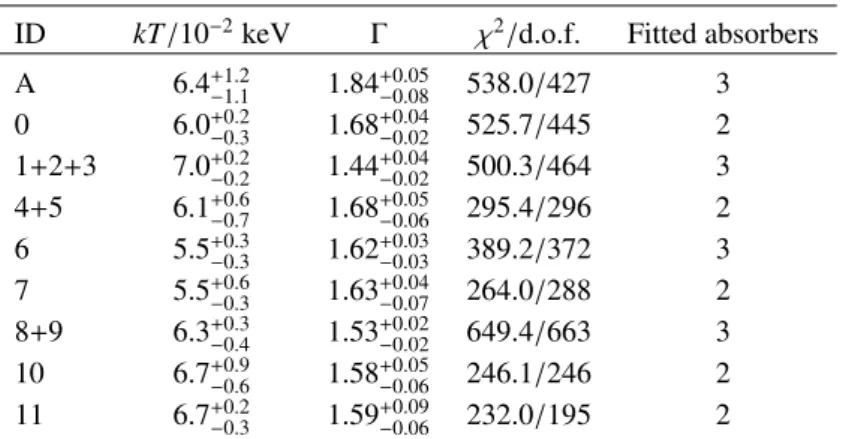
ID kT/10−2keV Γ χ2/d.o.f. Fitted absorbers A 6.4+1.2−1.1 1.84+0.05−0.08 538.0/427 3 0 6.0+0.2−0.3 1.68+0.04−0.02 525.7/445 2 1+2+3 7.0+0.2−0.2 1.44+0.04−0.02 500.3/464 3 4+5 6.1+0.6−0.7 1.68+0.05−0.06 295.4/296 2 6 5.5+0.3−0.3 1.62+0.03−0.03 389.2/372 3 7 5.5+0.6−0.3 1.63+0.04−0.07 264.0/288 2 8+9 6.3+0.3−0.4 1.53+0.02−0.02 649.4/663 3 10 6.7+0.9−0.6 1.58+0.05−0.06 246.1/246 2 11 6.7+0.2−0.3 1.59+0.09−0.06 232.0/195 2
Notes. The final χ2for the best-fit model of each observation is shown, as well as the number of absorbers fitted for each spectrum (see TablesB.1–
Appendix C: Comparison between XMM-Newton cameras
Fig. C.1.Best-fit values of the pn camera (blue squares), the MOS
cam-eras combined (red triangles), and pn and MOS data together (black circles) of the three parameters of Abs. 2. The star is the ASCA value. The parameters are in agreement within their errors at 90% confidence level. The horizontal black line represents the cosmological redshift of the source, zo= 0.144.
Appendix D: Spectra
time (yrs)
Fig. C.2.Best-fit values of the pn camera (blue squares), the MOS
cam-eras combined (red triangles), and pn and MOS data together (black circles) of the three parameters of Abs. 3. The star is the ASCA value. The parameters are in agreement within their errors at 90% confidence level. The horizontal black line represents the cosmological redshift of the source, zo= 0.144. 10−4 10−3 n o rm a liz e d c o u n ts s − 1 k e V − 1 c m − 2 1 0.5 2 5 1 1.5 ra ti o Energy (keV)
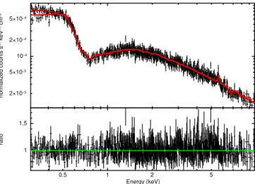
Fig. D.1.Spectrum and ratio of Obs. 0. The red line is the best fit.
10−5 10−4 2×10⁻⁵ 5×10⁻⁵ 2×10⁻⁴ 5×10⁻⁴ n o rm a liz e d c o u n ts s − 1 k e V − 1 c m − 2 1 0.5 2 5 1 1.5 ra ti o Energy (keV)
10−4 2×10⁻⁵ 5×10⁻⁵ 2×10⁻⁴ 5×10⁻⁴ n o rm a liz e d c o u n ts s − 1 k e V − 1 c m − 2 1 0.5 2 5 1 1.5 ra ti o Energy (keV)
Fig. D.3.Spectrum and ratio of Obs. 4+5. The red line is the best fit.
10−4 10−3 n o rm a liz e d c o u n ts s − 1 k e V − 1 c m − 2 1 0.5 2 5 1 1.5 ra ti o Energy (keV)
Fig. D.4.Spectrum and ratio of Obs. 6. The red line is the best fit.
10−4 2×10⁻⁵ 5×10⁻⁵ 2×10⁻⁴ 5×10⁻⁴ n o rm a liz e d c o u n ts s − 1 k e V − 1 c m − 2 1 0.5 2 5 0.8 1 1.2 1.4 ra ti o Energy (keV)
Fig. D.5.Spectrum and ratio of Obs. 7. The red line is the best fit.
10−4 2×10⁻⁵ 5×10⁻⁵ 2×10⁻⁴ 5×10⁻⁴ n o rm a liz e d c o u n ts s − 1 k e V − 1 c m − 2 1 0.5 2 5 1 1.5 ra ti o Energy (keV)
Fig. D.6.Spectrum and ratio of Obs. 8+9. The red line is the best fit.
10−4 2×10⁻⁵ 5×10⁻⁵ 2×10⁻⁴ 5×10⁻⁴ n o rm a liz e d c o u n ts s − 1 k e V − 1 c m − 2 1 0.5 2 5 0.8 1 1.2 1.4 ra ti o Energy (keV)
Fig. D.7.Spectrum and ratio of Obs. 10. The red line is the best fit.
10−4 2×10⁻⁵ 5×10⁻⁵ 2×10⁻⁴ 5×10⁻⁴ n o rm a liz e d c o u n ts s − 1 k e V − 1 c m − 2 1 0.5 2 5 0.8 1 1.2 1.4 ra ti o Energy (keV)