U
U
n
n
i
i
v
v
e
e
r
r
s
s
i
i
t
t
à
à
d
d
i
i
B
B
o
o
l
l
o
o
g
g
n
n
a
a
Dottorato di Ricerca in Geofisica
XXI Ciclo
Tesi di Dottorato
Settore scientifico-disciplinare di afferenza Geo/10
3D Probability Tomography: theoretical developments
and applications to high-resolution
geophysical prospecting
Dottorando:
Dr. Raffaele Alaia
Coordinatore:
Relatore:
Prof. Michele Dragoni Prof. Domenico Patella
Introduction...1
1. Multipole Geophysical Tomography...5
1.1 General theory ...5
1.2 The source pole occurrence probability ...8
1.3 The source dipole occurrence probability ...9
1.4 The source quadrupole occurrence probability ...10
1.5 The source octopole occurrence probability...11
2. Multipole Geoelectrical Tomography ...12
2.1 The basic geoelectrical theory ...12
2.2 The generalized formalism for geoelectrical method ...15
2.3 Synthetic examples ...19
2.4 A field example at Pompei ...25
2.4.1 Geoelectrical data acquisition, processing and pseudoimaging ...27
2.4.2 Result of the 3D probability tomography ...31
3. Multipole Gravity Tomography ...39
3.1 The basic gravity theory ...39
3.2 The generalized formalism for gravity...43
3.3 Synthetic examples ...45
3.3.1 The one-cube model...45
3.3.2 The sphere model...49
3.3.3 The rotated and tilted cube model ...52
3.3.4 The two prism model...54
3.4 A field example...57
4. Multipole Self-Potential Tomography...62
4.1 The basic Self Potential theory ...62
4.2 The generalized formalism for Self Potential...64
4.3 Synthetic examples ...67
4.4.1 The one-cube model...67
4.4.2 The single point charge model ...70
4.4.3 The rotated and tilted cube model ...73
4.4.4 The two prism model...76
4.5 A field example...78
Conclusion ...83
Appendix ...86
1
Introduction
During the last few years geophysical methods employed in underground exploration have been constantly and substantially evolving in both physical and technological aspects.
The geophysical prospecting methods can be divided, in the first instance, into two categories, artificial source and natural source. The artificial source methods are based on the study of the observed responses on the surface of the interested volume of ground to a physical stress artificially induced in the ground. For example, the geoelectric method takes in exam the electric properties of the subsoil by studying the flux of artificially injected currents, thus allowing the retrieval of information about the electric resistivity of the surveyed ground portion. It can successfully highlight even weak resistivity contrasts that buried objects create with the hosting background.
The natural source methods, instead, base their development on the study of the fields naturally found inside the earth, as e.g. the gravimetric method. By analysing the gravitational field, it allows the properties of the matter which originated the field to be detected and hence the mass distribution below the surface to be imaged.
In synthesis, the principal aim of the geophysical studies is to retrieve information about shape, location and physical characteristics of the investigated bodies. To this purpose, it is necessary to solve the so-called “inverse problem”, i.e. to determine the characteristic parameters of the buried structures, starting from a series of measures obtained on the surface. The solution to this problem is very complex because of the many solutions compatible with an acquired data set, indeed, different bodies can cause the same image on the surface.
The probability tomography approach allows the analysis of the experimental data without introducing some a priori information on the investigated structures. In the limits of the experimental accuracy, the probability tomography is able to give a geometrical representation of the buried sources of anomalies. Therefore, the main
2 difference with the classical inversion methods is the absence of any possibility to estimate the intrinsic physical parameters of the source bodies. In many near-surface applications, e.g. in archaeological prospection, this is not a serious limitation, since in most cases location and geometry of the sources are more than sufficient to resolve the practical problem. In the cases in which the knowledge of the intrinsic physical parameter of the bodies is essential, the results of the probability tomography can suitably used as robust geometrical constraints in any of the classical inversion routines.
Geophysical probability tomography (GPT) was proposed as an approach to virtually explore the subsoil in the search for the most probable localization of the sources of anomalies appearing in a field dataset collected in a given datum domain. It was originally formulated for the self-potential method [41,42] and then extended to the geoelectric [25,26,32], em induction [27], gravity [28,29] and magnetic [18,19,30] prospecting methods. In all of these formulations, the buried bodies responsible for the observed anomalies were considered as aggregates of small cells, definitively assimilated to poles. A pole was thus assumed to represent the physical centre of a small cell with a constant electric charge density in the self-potential and, mass density in gravity and resistivity in geoelectrics. GPT sensitivity and resolution power have been and are still widely and successfully tested on synthetic and experimental data in many application fields [6,7,8,12,13,24,43,53] .
An extension of the GPT theory has been recently proposed [32] by postulating that some given geophysical dataset can be viewed as the simultaneous response of a double set of buried physical sources, say poles and dipoles. In this new formulation, while poles hold the original meaning as explained above, dipoles, instead, are assumed to simulate sharp boundary elements. The two-source GPT approach has been shown to provide a more reliable depiction of the most probable spatial collocation and extent of source bodies [1].
This thesis is composed of two parts. The first part , theoretical and methodological, has been addressed to the development of the GPT method to multipole source analysis in order to obtain more information on the shape and the position of the sources of the experimentally detected anomalies.
3 We develop the theory of the generalized 3D GPT to image source poles, dipoles, quadrupoles and octopoles, from a generic geophysical vector or scalar field dataset [2,3,4].
The generalised 3D GPT method is described by first assuming that any geophysical field dataset can be hypothesized to be caused by a discrete number of source poles, dipoles, quadrupoles and octopoles.
Then, the theoretical derivation of the source pole occurrence probability (SPOP) and source dipole occurrence probability (SDOP) tomography, previously published in detail for single geophysical methods, is symbolically restated in the most general way. Finally, the theoretical derivation of the source quadrupole occurrence probability tomography (SQOP) and source octopole occurrence probability tomography (SOOP) are given following a formal development similar to those of the SPOP and SDOP tomography.
These elementary sources are used to image, in the most complete way and without any a priori assumption, shape and position of the most probable anomaly source bodies, by picking out the location of the centres and of peculiar points of the boundaries, such as corners, wedges and vertices. In this new formulation, poles and dipoles still have the original meaning to represent centres and boundaries, respectively, of elementary bodies with constant constitutive parameters, while quadrupoles and octopoles are assumed to simulate sharp corners, wedges and vertices elements. The purpose of multipole analysis is to improve the resolution power of geophysical methods, using once more probability as a suitable paradigm allowing all possible equivalent solutions to be included into a unique 3D tomography image.
The second part is dedicated to the application of the developed theory to synthetic data for method testing and to real data for a comparison with the previous inversion results. The innovative aspects and the improvements of this method for the 3D tomographic imaging of buried targets is discussed in detail.
The applications fields have been archaeology for near-surface analysis and vulcanology for deep analysis.
In particular, for the near-surface analysis in archaeological prospection, a geoelectrical survey was planned in an unexplored site of the archaeological park of Pompei.
4 For the deep analysis in volcanological prospection, the experimental data taken into consideration are related to a gravity survey carried out in the volcanic area of Mount Etna (Sicily, Italy), and an SP dataset collected in the Mt. Somma-Vesuvius volcanic district (Naples, Italy).
5
1. Multipole Geophysical Tomography
1.1 General theory
Consider a reference coordinate system with a horizontal (x,y)-plane and the z-axis positive downwards, and a 2D datum domain S as in figure 1.1. The S-domain is generally a non-flat ground survey area characterised by a topographic function z(x,y).
Let A(r) be a vector anomaly function at a set of datum points r(x,y,z), with rS, we assume that A(r) can be discretised as
1 1 ( ) ( , ) ( ) ( , ) M N u u m m m n n n m n
A r p P s r r d L s r r 1 1 ( ) ( , ) ( ) ( , ) G H uv uv uvw uvw g g g h h h g h
q S s r r
o C s r r (1.1)i.e. as a sum of effects due to:
- a set of M poles, the mth element of which is located at rm(xm,ym,zm) and has
strength pmPm, where pm and Pm are the pole moment and a point operator
zero-order tensor, respectively;
- a set of N dipoles, whose nth element is located at rn(xn,yn,zn) with strength
( u n u n L d ) (u=x,y,z), where u n d and u n
L are the dipole moment and a line operator first-order tensor, respectively;
- a set of G quadrupoles, whose gth element is located at rg(xg,yg,zg) with strength
uv g uv g S q (u,v=x,y,z), where uv g q and uv g
S are the quadrupole moment and a square operator second-order tensor, respectively;
6 - a set of H octopoles, whose hth element is located at rh(xh,yh,zh) and has strength
uvw h uvw h C
o (u,v,w=x,y,z), where uvw h
o and uvw h
C are the octopole moment and a cube operator third-order tensor, respectively.
The dot in the definition of the source strength tensors indicates inner product. The operator tensors P, Lu, Suv and Cuvw (u,v,w=x,y,z) are explicated in figure 1.2 .
The effect of the M, N, G and H source elements at a point rS is determined by the same kernel function s(r,ri), (i=m,n,g,h).
Figure 1.1 The datum domain (S-domain) generating the A(r) map on top. The (x,y)-plane is placed at
sea level and the z-axis points into the earth.
We define the information power , associated with A(r), over the surface S as
S
dS
7 which, using eq. 1.1, is expanded as
1 Λ ( , )d M m m m S p S
A r s r r
1 , , ( , ) d N u n n n u x y z S n d S u
A r s r r
2 1 , , , , ( , ) G g uv g g u x y z v x y z S g g q dS u v
A r s r r
3 1 , , , , , , ( , ) H uvw h h h u x y z v x y z w x y z S h h h o dS u v w
A r s r r (1.3)Figure 1.2 Explicit representation of the symbolic tensor operators appearing in the definition of the
8 1.2 The source pole occurrence probability
We consider a generic mth integral of the first sum in eq. 1.3 and apply Schwarz’s inequality, thus obtaining
2 ( ) ( , m) S dS
A r s r r 2( ) 2( , m) S S A dV s dS
r
r r (1.4)where A(r) and s(r,rm) are the modulus of A(r) and s(r,rm), respectively.
Inequality 4 is used to define a source pole occurrence probability (SPOP) function [2,28] as
( ) ( ) ( , ) p p m m m S C dS
A r s r r (1.5) where 1/ 2 ( ) 2 2 ( ) ( , ) p m m S S C A dS s dS
r r r (1.6)The 3D SPOP function, which satisfies the condition 1m(p)1, is given as a
measure of the probability of a source pole of strength pm placed at rm, being
responsible for the observed anomaly field A(r). The m( P) function can readily be computed knowing the mathematical expression of the function s(r,rm), which is given
the role of source pole scanner.
For computational purposes, we assume the projection of S onto the (x,y)-plane can be fitted to a rectangle R of sides 2X and 2Y along the x- and y-axis, respectively. Using the topography surface regularization factor g(z) given by [28,29]
9
2 2
1/2 ) / ( ) / ( 1 ) (z z dx z dy g t (1.7)eq. 1.5 is definitely written as follows
( ) ( ) ( , ) ( ) X Y p p m m m X Y C g z dxdy
A r s r r (1.8) with ( ) 2 ( ) ( ) X Y p m X Y C A g z dxdy
r 2 / 1 2 ) ( ) , (
X X Y Y m g zdxdy s rr (1.9)1.3 The source dipole occurrence probability
We take a generic nth integral of the second sum in eq. 1.3 and apply, as previously, Schwarz’s inequality to each u-component (u=x,y,z). We can thus define a source dipole
occurrence probability (SDOP) function [2,18] as
( ) ( ) , , ( , ) ( ) X Y d d n n u n u n X Y C g z dxdy u
A r s r r (1.10) with
( ) , ( ) X Y d n u X Y C g z dxdy
A r 1/ 2 2 ( , ) ( ) X Y n n X Y g z dxdy u
s r r (1.11)10 where surface regularization has been accounted for.
Also ( ) ,
d u n
falls in the range [-1,1]. Thus, at each rn, 3 values of (,)
d u n
can be computed. They are interpreted to give a probability measure, with which a single source dipole located at rn can be retained responsible of the whole A(r) field.
Each first derivative of s(r,rn) takes the role of source dipole scanner.
1.4 The source quadrupole occurrence probability
Accordingly, we consider now a generic gth integral of the third sum in eq. 1.3 and apply again Schwarz’s inequality to each uv-element (u,v=x,y,z), which is used to define the source quadrupole occurrence probability (SQOP) function [2] as
2 ( ) ( ) , , ( , ) ( ) ( ) X Y g q q g uv g uv g g X Y C g z dxdy u v
A r s r r (1.12) with ( ) 2 , ( ) ( ) X Y q g uv X Y C A g z dxdy
r 1/ 2 2 2 ( , ) ( ) X Y g g g X Y g z dxdy u v
s r r (1.13)As previously, also the 3D SQOP function falls in the range [-1,1]. Thus, at each rg,
9 values of ( ) ,
q uv g
are taken as a measure of the probability for a quadrupole source located at rg, to be responsible of the A r dataset. Since ( ) Suvg is a symmetric square
tensor, it follows ( ) , ) ( , q vu g q uv g
. Hence, at each rg, the 3 diagonal plus the 3 right-up or
left-down off-diagonal terms of ( ) ,
q uv g
are sufficient.
11 1.5 The source octopole occurrence probability
Finally, we consider a generic hth integral of the fourth sum in eq. 1.3 and apply again Schwarz’s inequality to each uvw-term (u,v,w=x,y,z), allowing a source octopole
occurrence probability (SOOP) function [3,4] to be defined as
3 ( ) ( ) , , ( , ) ( ) ( ) X Y o o h h uvw h uvw h h h X Y C g z dxdy u v w
A r s r r (1.14) with ( ) 2 , ( ) ( ) X Y o h uvw X Y C A g z dxdy
r 1/ 2 2 3 ( , ) ( ) X Y h h h h X Y g z dxdy u v w
s r r (1.15)As previously, the 3D SOOP function falls in the range [-1,1]. At each rh, 27 values
of ( ) ,
o h uvw
may be calculated, which are interpreted as a measure of the probability of a single source octopole located at rh, being responsible of the whole A r dataset. ( )
However, as we are interested in finding only the position of the vertices of a source body, we will limit our analysis only to the SOOP function with uvw.
12
2. Multipole Geoelectrical Tomography
2.1 The basic geoelectrical theory
The fundamental physical law used in resistivity surveys is Ohm’s Law that governs the flow of current in the ground. The equation for Ohm’s Law in vector form for current flow in a continuous medium is given by
J = σ·E (2.1) where σm is the conductivity of the medium, J (A/m2) is the current density and E (V/m), is the electric field intensity. In practice, what is measured is the electric field potential. We note that in geophysical surveys the medium resistivity ρ, which is equals to the reciprocal of the conductivity ρ = 1/σ, is more commonly used. The relationship between the electric potential U (Volt) and the field intensity is given by
E = -U (2.2)
Combining equations (2.1) and (2.2), we get
J = -σU (2.3)
In almost all surveys, the current sources are in the form of point sources. In this case, over an elemental volume V surrounding the a current source I, located at (xs,
ys,zs) the relationship between the current density and the current [11] is given by
·J ( s) ( s) ( s) I x x y y z z V (2.4)
13 where is the Dirac delta function. Equation (2.4) can then be rewritten as
, ,
, ,
( ) ( ) ( ) σ x y z U x y z I x xs y ys z zs V (2.5)This is the basic equation that gives the potential distribution in the ground due to a point current source. A large number of techniques have been developed to solve this equation. This is the “forward” modeling problem, i.e. to determine the potential that would be observed over a given subsurface structure. Fully analytical methods have been used for simple cases, such as a sphere in a homogenous medium or a vertical fault between two areas each with a constant resistivity. For an arbitrary resistivity distribution, numerical techniques are more commonly used.
We consider simplest case with a homogeneous subsurface and a single point current source on the ground surface (figure 2.1). In this case, the current flows radially away from the source, and the potential varies inversely with distance from the current source. The equipotential surfaces have a hemisphere shape, and the current flow is perpendicular to the equipotential surface. The potential in this case is given by
2 ρ I U r πr (2.6)where r is the distance of a point in the medium (including the ground surface) from the electrode.
In practice, all resistivity surveys use at least two current electrodes, a positive current and a negative current sources and two electrodes of measurement (for the potential difference). A typical arrangement with 4 electrodes is shown in figure 2.2.
The potential difference is then given by
N B N A M B M A BN AN BM AM N M r r r r π ρ I U U U U U Δ 1 1 1 1 2 (2.7)14 The above equation gives the potential that would be measured over a homogenous half space with a 4 electrodes array.
Actual field surveys are invariably conducted over an inhomogenous medium where the subsurface resistivity has a 3-D distribution.
Figure 2.1 The flow of current from a point current source and the resulting potential distribution.
The resistivity measurements are still made by injecting current into the ground through the two current electrodes (A and B in figure 2.2), and measuring the resulting voltage difference at two potential electrodes (M and N). From the current (I) and potential (UMN) values, an apparent resistivity ( ) value is calculated. a
I ΔU K
ρ g MN (2.8)
15 Figure 2.2 Example surface electrode configurations
The calculated resistivity value is not the true resistivity of the subsurface, but an “apparent” value that is the resistivity of a homogeneous ground that will give the same resistance value for the same electrode arrangement. The relationship between the “apparent” resistivity and the “true” resistivity is a complex relationship. To determine the true subsurface resistivity from the apparent resistivity values is the “inversion” problem.
2.2 The generalized formalism for geoelectrical method
To approach the geoelectric problem, we assume, for the sake of simplicity and without loss of generality, that the volume V in figure 2.3 is a rectangular prism with its upper surface S representing a portion of a flat ground level. We also assume that the apparent resistivity values are attributed to the nodes of a 3D regular grid filling V, each identified by a tern of integer numbers i,j,k specifying the position along the x,y,z axes, respectively, originating from a point arbitrarily chosen over S.
16 Figure 2.3 The 3D datum domain, characterized by irregular boundary surfaces. The
(x,y)-plane is placed at sea level and the z-axis points into the earth .
In geoelectrics, the anomaly and kernel functions are scalar quantities. In order to obtain the explicit expressions of A(r) and s(r) we proceed as follows. We consider a homogeneous half-space with resistivity 0, where a perturbation of resistivity, say
m=m-00, is introduced at a generic single pole with coordinates (xm,ym,zm). The
apparent resistivity a(i,j,k) of such a weakly perturbed model, where neither dipole nor
quadrupole effects can generate, is approximated by a Taylor’s expansion stopped to Born approximation, i.e. to the first derivative term, as
m m a a m k j i k j i 0 ) , , ( ) , , ( 0 (2.9)
17 0 ) , , ( ) , , ( ) ( i j k i j k A r a a (2.10)
and the kernel function as
0 ) , , ( ) , ( m m a m k j i s r r (2.11)
In practice, the geoelectrical anomaly function a(i,j,k) is calculated by subtracting
from the measured apparent resistivities a(i,j,k) a reference uniform resistivity, which
can be either the background resistivity of the medium hosting the target bodies, if known, or, alternatively, any other reasonable value, as, e.g., the average apparent resistivity. The geoelectrical anomaly function has thus a quite obvious relative meaning, as it represents the responses of whatever bodies which are assigned true resistivities differing from 0.
For the calculation of the kernel function a(i,j,k)/mm=0, (appendix a), the
reader can refer to an expanded version reported in previous papers [1,2,26], which was derived using the Frechet derivative [40] of the geoelectric potential, obtained by Loke and Barker [23].
Once the key functions A(r) and s(r) have been defined, we can readily apply the general 3D GPT theory, previously exposed, by admitting that the anomaly sources responsible of any a(i,j,k) dataset can generally be made of M poles, each with its
own strength m (m=1,2,..,M), N dipoles, each with its own 3 moment vector
components nun (n=1,2,..,N; u=x,y,z), and G quadrupoles, each with its own 9
moment tensor elements gugg (g=1,2,..,G; u,=x,y,z). Eq. 1.1 is therefore
explicated as follows
M m m a m a m k j i k j i 1 0 ) , , ( ) , , ( 0 2 1 , , ( , , ) n N a n n n ν x y z n n i j k u v
0 3 1 , , , , ( , , ) g G a g g g g u x y z x y z g g g i j k u u
(2.12)18 Skipping all intermediate steps, we directly arrive at the explicit expressions of the geoelectrical SPOP, SDOP and SQOP functions, using a discretised version of the integrals appearing in the pair of eq.s 1.8 and 1.9, eq.s 1.10 and 1.11 and eq.s 1.12 and 1.13. The geoelectrical 3D SPOP function is given as [1]
0 , , ) ( ) ( ( , , ,) ) , , (
m k j i m a a P m P m k j i k j i C (2.13) with 2 / 1 , , , , 2 2 ) ( 0 ) , , ( ) , , (
i jk
i jk m a a P m m k j i k j i C (2.14)The geoelectrical 3D SDOP function is given as [1]
0 2 ( ) ( ) , , , , ( , , , ) ( , , ) n D D a n u n u i j k a n n i j k C i j k
, (u=x,y,z) (2.15) with 0 1/ 2 2 2 ( ) 2 , , , , , ( , , ) ( , , ) n D a n u i j k a i j k n n i j k C i j k u
, (u=x,y,z) (2.16)Finally, the geoelectrical 3D SQOP function is given as [2]
0 , , 3 ) ( , ) ( , ) , , , ( ) , , (
g k j i g g g a a Q u g Q u g u k j i k j i C , (u,=x,y,z) (2.17)19 with 2 / 1 , , , , 2 3 2 ) ( , 0 ) , , ( ) , , (
i jk
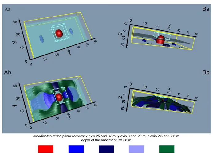
i jk g g g a a Q u g g u k j i k j i C , (u,=x,y,z) (2.18) 2.3 Synthetic examplesWe show a few simple synthetic examples in order to highlight the main aspects of the SQOP tomography. In all of the examples, the new SQOP tomography will always be compared with the SPOP and SDOP tomographies in order to elicit complementary aspects. The first case is a rectangular prism with resistivity of 5000 m , immersed in a homogeneous half-space with resistivity of 500 m, reproduced in all templates of figures 2.4a and 2.4b with light blue lines, where the bigger prism with yellow lines represents the datum volume V, and columns A and B display the same results under different viewing angles.
20 Figure 2.4 (a) The SPOP, SDOP and SQOP 3D GPT for a rectangular prism of 5000 m (bordered by light blue lines) and spatial location as in legend, immersed in a homogenous half space of 500 m. The larger prism bordered by yellow lines is the 3D datum domain. Scale of axes is in m. For the isosurfaces bounding the coloured nuclei, containing the SPOP, SDOP and SQOP primary MAV, see table 2.1 appendix b. (b) The SPOP, SDOP and SQOP 3D GPT for a rectangular prism of 5000 m (bordered by light blue lines) and spatial location as in legend, buried in a homogenous half space of 500 m. The prism with yellow borders is the datum domain. The scale of axes is in m. For the isosurfaces bounding the coloured small (row a) and big (row b) nuclei, containing the SPOP, SDOP and SQOP MAV, see table 2.2 appendix b.
21 In figure 2.4a the m( )P , n u(D,) (u=x,y,z ) and g xy( )Q, primary maximum absolute values (MAV) are considered, which, for the sake of visibility, are each represented by a nucleus bounded by the isosurface relative to 95% of the corresponding primary MAV (table 2.1 appendix b). Row a refers to the combination of SPOP and SDOP nuclei, which confirm known results [32].
In fact, a m( )P nucleus, a pair of
( ) , D n x and (, ) D n y nuclei and a (, ) D n z appear in correspondence to the centre, close to the lateral faces oriented along the x- and y-axes and at the base of the prism, respectively.
Row b shows the position of the six SQOP nuclei, drawn as before by considering the isosurface relative to 95% of the corresponding primary MAV (table 2.1 appendix b). Of all of them, only the g xy( )Q, nuclei are assumed to give additional information. In fact, they appear located close to the prism basal vertices, whereas the other ( )
,
Q g u
nuclei confirm the position of the prism central axis and its lateral and bottom faces.
Finally, row c shows the set of m( )P , n u(D, ) (u=x,y,z ) and g xy( )Q, nuclei, which are assumed to provide a sufficient set of information as to the prism spatial location. One gets the impression that the m( )P nucleus locates right at the centre of the prism, whereas the n u(,D) (u=x,y,z ) and g xy( )Q, nuclei appear confined around the base of the prism. Thus, the whole set of nuclei in figure 2.4a is interpreted as the simplest combination of pole, dipole and quadrupole source elements with maximum occurrence probability, out of the group of all equivalent, more complex multipole source combinations providing the same apparent resistivity dataset within V.
In order to see whether there is a way to highlight the 3D geometry of the source body, row b in figure 2.4b shows the m( )P , n u(D,) (u=x,y,z ) and g xy( )Q, isosurfaces relative to a percentage of the primary MAV as listed in table 2.2 appendix b. Except for the
( )P m
nucleus, for which the same reduction as before has been used, all other reductions have been set at 50%, so chosen as to fit to the following criterion. By gradually decreasing the percentage at steps of 5% from 95%, we have observed the growth of a bump in the isosurfaces, peaking up to a maximum and then gradually flattening, till vanishing. We have assumed the percent value corresponding to the observed maximum bump peaking.
22 Figure 2.4 (b) (Continued.)
This approach is nothing but a quick inspection of the presence of secondary MAV. The picture thus obtained is compared with the previous one drawn in row c of figure 2.4a, and replicated in row a of figure 2.4b. The peaking bumps are all directed topwards, with those of ( )
,
D n u
(u=x,y ) spreading against the lateral faces, and those of climbing ( ),
Q g xy
along the vertical edges of the prism.
As a second example, we consider the situation where the same prism with a resistivity of 5000 m as before emerges from a substratum with the same resistivity into a top layer of 500 m. Figure 2.5 shows the results of the new simulation. In detail, row a shows the m( )P , n u(D,) (u=x,y) and g xy( )Q, nuclei bounded by isosurfaces relative to 95% of the corresponding primary MAV (see table 2.2 appendix b).
23 Figure 2.5 The SPOP, SDOP and SQOP 3D GPT for a rectangular prism of 5000 m (bordered by light blue lines) and spatial location as in legend, immersed in a two-layer host medium with an overburden of 500 m and substratum of 5000 m. The prism with yellow borders is the datum domain. Scale of axes is in m. For the isosurfaces bounding the coloured small (row a) and big (row b) nuclei, containing the SPOP, SDOP and SQOP MAV, see table 2.2 appendix b.
Compared with the previous case, we do not recognize now any relation of the nuclei with characteristic points of the prism, due to the presence of the high-resistivity basement. Once again, we must retain that this set of primary MAV nuclei represents the simplest array of source elements with maximum occurrence probability, within the class of equivalent arrangements. Row b shows the m( )P , n u(D,) (u=x,y) and g xy( )Q, isosurfaces relative to the percentages of the primary MAV listed in table 2.2 Appendix B, obtained by the maximum bump peaking criterion previously illustrated.
Row b shows a clear smooth version of the prism-basement geometry, rather distorted at the margins due to the finite extent of V. The influence of the finite extent of the data volume is a topic poorly investigated in most modelling and inversion
24 approaches. We continue our simulation analysis by proposing a more complex target structure, made of two separated prisms, with different sizes and collocation, without and with basement. The results are depicted in figures 2.6 and 2.7 for the two-prism structure in a homogeneous half-space and in a two-layer host medium, respectively. For both simulations, the same comments as in the previous corresponding cases can be made, except for the evident loss of symmetry of the isosurfaces, due to the different size and collocation of the two prisms.
Figure 2.6 The SPOP, SDOP and SQOP 3D GPT for a two-prism model of 5000 m (bordered by light blue lines) and spatial location as in legend, immersed in a homogenous half space of 500 m. The larger prism with yellow borders is the 3D datum domain. Scales are in m. For the isosurfaces bounding the coloured small (row a) and big (row b) nuclei, containing the SPOP, SDOP and MAV, see table 2.2 appendix b.
25 Figure 2.7 The SPOP, SDOP and SQOP 3D GPT for a two-prism model of 5000 m (bordered by light blue lines) and spatial location as in legend, immersed in a two-layer host medium with overburden of 500 m and substratum of 5000 m. The larger prism bordered by yellow lines is the 3D datum domain. The scale of the three coordinate axes is in m. For the isosurfaces bounding the coloured small (row a) and big (row b) nuclei, containing the SPOP, SDOP and SQOP MAV, see table 2.2 appendix b.
2.4 A field example at Pompei
.
We show the results obtained from the application of an advanced geoelectrical tomography survey performed in an unexplored site of the archaeological park of Pompei, aiming at identifying anomalies ascribable to remains of walls and roads, according to the expectation of the local archaeological authority.
The Roman town of Pompei, located 30 km SE of Naples, developed on a flat topographical surface gently degrading towards the Gulf of Naples, created by the
26 Vesuvius activity, which had prior deposited in this sector an alternating sequence of fall and flow pyroclastic products. Then, the 79 AD Vesuvius eruption completely destroyed the Roman town, covering it with even more than 10 m of pyroclastic fall products. Nowadays, only a little amount of the vestiges of the ancient Pompeian civilization has been brought to light.
The study area is located in the Regio III sector of the archaeological park (figure 2.8), on a locally flat topographic high created by the 79 AD pyroclastic deposits (figure 2.9a), placed at no more than 6 m above the original ground level of the ancient town, judging from the adjacent visible ruins (figure 2.9b).
Figure 2.8 Plan view of a portion of the Pompei archaeological park. The rectangle in the Regio III sector
is the area surveyed by the geoelectrical method. The top right corner of the rectangle is assumed to be the origin of the local reference coordinate system.
27 Figure 2.9 (a) The rectangular geoelectrical survey area in the Regio III sector of the Pompei
archaeological park. The far-field left corner corresponds to the top right corner of the rectangle sketched in figure 2.8 and is assumed to be the origin of the local reference coordinate system. (b) Pompeian exposed ruins adjacent to the top longer side of the rectangle sketched in figure 2.8.
2.4.1 Geoelectrical data acquisition, processing and pseudoimaging
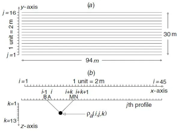
Figure 2.9a shows the rectangular area of 2820 m2 (94 m 30 m), where 16 parallel profiles of 94 m of length equispaced by 2 m were programmed. The longer side of the rectangle was oriented N60°E, normal to the main axis of the nearby excavated Roman
insulae (figure 2.8). This axis was thus assumed as the strike of a prevailing 2D
resistivity structure expected under the chosen rectangle. For this reason, the dipole-dipole (DD) electrode array, notoriously most sensitive to lateral resistivity contrasts [34], was run along each line according to the well known pseudosection data acquisition technique.
A programmable resistivity-meter was used, which allowed up to 23 simultaneous voltage measurements for every current injection, by setting the maximum standard deviation at 3% and selecting the number of stacking cycles between 3 and 10 for random noise attenuation. The spreads of the emitting and receiving dipoles and the advancing step along the profiles were fixed at 2 m. The distance between the centres of the dipoles was expanded from an initial spacing of 4 m up to 28 m, thus reaching the maximum pseudodepth of 14 m starting from 2 m and going down by 1 m every 2 m of
28 spacing increase. 507 DD apparent resistivity determinations were thus realized along each profile for a total of 8112 data collected inside the whole rectangle.
Figure 2.10 resumes the DD data acquisition procedure. As said, it consists of a sequence of parallel profiles on a flat ground surface, identified by the index j=1,2,..,16, as in figure 2.10a. The generic jth profile is then considered in detail in figure 2.10b, where the emitting (AB) and receiving (MN) dipoles are identified by the indices
i=1,2,..,45 and k=1,2,..,13, and the depth of attribution of the apparent resistivity value
(pseudodepth) by the index k=1,2,..,13. Hence, each apparent resistivity value is a function of the three indices, say a(i,j,k).
Figure 2.10 The dipole–dipole (DD) geoelectrical procedure in the rectangular survey area of figure 2.8 .
(a) Plan view of the regular DD profile distribution in the area; (b) the pseudodepth data attribution technique along a DD profile.
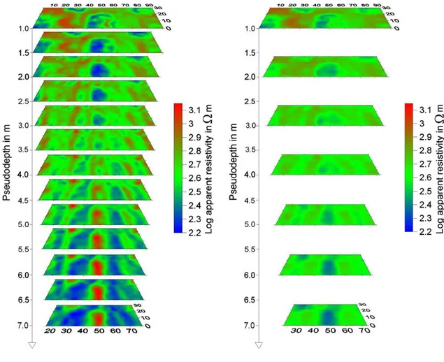
Figure 2.11a displays a sequence of horizontal slices, in each of which the common logarithm of the DD apparent resistivities at the same pseudodepth are contoured. The slices were drawn using the whole dataset of the 16 parallel profiles. This slice sequence gives a quick view of the degree of inhomogeneity in the subsoil, which in the
29 pseudodepth range from 2 m down to about 8 m seems to dominate along the x-axis, i.e. the direction of the long side of the survey rectangle (figure 2.8). In the following pseudodepth range from 9 m down to 14 m, the DD apparent resistivity pattern radically changes showing the tendency to homogenize towards low apparent resistivity values, except for two evident anomalous highs, of which the biggest one dominates in the whole central area and the other one is confined in the top marginal area in the left-hand sector of the slices.
Figure 2.11 The DD (a) and Wenner (b) pseudoslice imaging of the apparent resistivity values collected
in the rectangular survey area of figure 2.8.
The DD apparent resistivity pattern in the near-surface pseudodepth range can qualitatively be interpreted as the geoelectric signature of archaeological remains, in accordance with the initial hypothesis of anomalies expected to conform to a probable S30°E continuation of the wall-and-road mesh appearing aside in the partially excavated
30 range seems, instead, to represent the relatively less resistive nature of the local substratum. It appears to expand under the whole survey area, except for the mentioned positive nuclei, which are suspected to be ghost anomalies, typical of the dipole-dipole array, due to the diagonal downward dragging effect of shallow resistive anomalies, also known as the inverted V-shaped effect.
To better visualize this effect, figure 2.12 shows the pseudosections relative to two profiles selected in correspondence with the top marginal and the bigger central positive anomaly, respectively. These anomalies here appear as the result of a focalization of two nearby inverted V-shaped dragging effects, right where the inner tails intersect. Nonetheless, to take a final decision, we carried out in the whole area a further geoelectric survey, using the Wenner array, which is not influenced by dragging effects. An approach similar to the DD technique was used, consisting in expanding the Wenner spacing, equal to one third of the distance between the external A and B current electrodes, by multiples of 2 m, starting from 2 m up to 14 m. The Wenner apparent resistivity values conventionally are attributed along the vertical axis through the centre of the array at a pseudodepth set equal to the array spacing.
Figure 2.12 DD pseudosections across the profiles at y = 2m (j= 2)and y = 28m (j= 15) cutting the
pseudoslice at the pseudodepth of 7 m (k = 13).
Figure 2.11b displays the sequence of horizontal slices so obtained, in each of which the common logarithm of the Wenner apparent resistivities at the same pseudodepth are contoured. No positive anomaly appears in the critical zones, at pseudodepths
31 comparable with those in figure 2.11a. Hence, we conclude that the deep DD positive nuclei in figure 2.11a are likely to be considered ghost anomalies.
It is finally worth noticing the less pronounced selectivity power of the Wenner array with respect to the DD array. The shallow anomalies of potential archaeological interest appear in figure 2.11b less articulated and more rapidly vanishing versus depth than the corresponding anomalies in figure 2.11a. This is the reason why we have definitely focused our attention only on the DD survey.
A DD apparent resistivity imaging like that in figure 2.11a has, however, only a rough relationship with the true resistivity structure, whose localization is the ultimate scope of this survey. In fact, shape and amplitude of the anomalies in figure 2.11a strictly represent the shift among different DD apparent resistivity values, each depending not only on the true resistivity distribution, but also on the array stepping used to sense the subsoil. In order to remove this last effect and get a more realistic imaging of the buried structures from the apparent resistivity dataset, we have applied the 3D probability tomography method [26] of which we give in the following section an extension according to the 3D DD data acquisition technique used in this survey. Probability tomography was originally proposed for the self-potential method [41,42], and very recently applied also to the magnetic method [30].
2.4.2 Result of the 3D probability tomography
Figure 2.13 shows the 3D geoelectric source pole tomography, represented as a sequence of slices at increasing depth from 2 m bgl down to 6.5 m bgl.
32 Figure 2.13 The near-surface 3D source pole tomography of the DD apparent resistivity values collected
in the rectangular survey area of figure 2.8.
We have deliberately chosen this depth interval, because, as previously outlined, it is likely to represent the buried environment thickness of archaeological interest. In fact, all SPOP nuclei potentially associable to archaeological bodies appear in this range. Firstly, we notice the presence of positive nuclei, mostly aligned along the y-axis, representing the zones where higher is the probability to find true resistivities exceeding the reference value, which was taken equal to the mean apparent resistivity of 432.5 m, whose common logarithm is 2.64. The maximum SPOP value of each of these positive nuclei is met at a depth around 3.5 m bgl, which is assumed as the depth of the centre of mass of the more resistive bodies. From the archaeological point of view, these masses can be associated with remains of walls and/or heaps of collapsed stone blocks.
33 Another clear signal is the central large negative nucleus, which of course identifies a zone where the probabilities to find true resistivities lower than the reference value are higher. The maximum absolute value within this negative nucleus is found again at a depth around 3.5 m bgl. From the archaeological point of view, we can now associate this less resistive volume to accumulation of wet volcanic products filling an originally open air space, very likely a peristilio, i.e. a home court with columned portico. Less intense are two other negative nuclei, one visible since the shallowest slice, around the point x=32 m and y=28 m, and the other starting from the slice at 2.5 m of depth, around the point x=70 m and y=8 m. As the previous negative nucleus, also the two smaller cores may be ascribed to accumulations of wet volcanic products filling again originally open spaces, very likely associable now to the presence of roads, as the cores seem to assume a narrow elongated shape from 4.5 m of depth down to 5.5-6 m. They finally tend to be fully absorbed inside deeper and much larger negative nuclei, visible in the far-surface tomography depicted in figure 2.12, very likely representing the virgin volcanic top soil existing before the 79 AD eruption.
Figure 2.14 The far-surface 3D source pole tomography of the DD apparent resistivity values collected in
34 To enhance the previous archaeological tentative interpretation of the anomalies emerged from the 3D tomographic analysis, we show in figure 2.15 how the SPOP nuclei spread over the most significant slice at 3.5 m of depth correlate with the traces of the remains so far explored within the insulae viii, ix and x inside the Regio III sector of the park.
It is worthwhile to observe how the 3D probability tomography method behaves in presence of ghost anomalies, like e.g. the deep positive anomaly appearing in the central part of the deep pseudoslices in figure 2.11a. This ghost effect has almost completely dropped out as no positive nucleus appears in the same region across the bottom depth range in figure 2.8. This is a further evidence of the filtering power of the probability tomography method, already tested in previous applications [26,27].
Figure 2.15 The investigated area in the archaeological park of Pompei with the SPOP tomographic slice
35 Figure 2.16 shows the 3D source dipole tomography, given as a sequence of slices from 2 m down to 6.5 m bgl. Owing to the vector character of the dipole, the 3D SDOP analysis is performed for each scalar dipole component along its relative reference axis.
Figure 2.16 The 3D source dipole tomography of the DD apparent resistivity values collected in the
survey area of figure 2.8. Tomography of the x-component (a), the y-component (b) and the z-component (c) of the dipole sources.
36 We recall that the presence of a SDOP nucleus along a given axis marks the passage from one to another different resistivity along that direction, thus providing an indication about the position of a resistivity boundary. Since in the present application the expected geometry of the concealed targets should nearly conform to right prismatic bodies with corners parallel to the x,y,z axes, the presence of a pair of adjacent SDOP nuclei with opposite sign occurring along one axis can be a useful indicator of the body size along that axis. Moreover, as it regards the sign of a SDOP nucleus we recall that, moving along the positive direction of a system axis, a positive sign of the relative dipole component marks the transition from a lower to a higher resistivity value across the boundary that the nucleus highlights, and the reverse for a negative sign.
Figure 2.16a refers to the x-component of the dipole sources. The sequence of pairs of opposite sign SDOP nuclei, elongated along the y-axis, is a clear evidence of where the transition from the resistive blocks to the conductive filled spaces and vice versa are most likely located along the x-axis. A similar conclusion can be reached along the y-axis looking at figure 2.16b, which shows the SDOP analysis of the y-component of the dipole sources, now characterized by less intense, but more concentrated nuclei. At last, figure 2.16c refers to the z-component of the dipole sources. This last representation is quite similar to the SPOP tomographic sequence in figure 2.16 as far as the shallow nuclei of archaeological concern are considered. The only difference, apart from the expected sign inversion, is that the nuclei of both signs are all shifted downwards, and their maximum absolute values are met around 5-6 m of depth bgl, i.e. approximately at the depth of the ancient ground level, amply visible north of the surveyed area (figure 2.9b).
Figure 2.17 shows the SPOP, SDOP and SQOP 3D tomographies obtained at Pompei, where, in order to put in evidence a source geometry as close as possible to the expected targets, only the m( )P , n u(D, ) (u=x,y,z) and g xy( )Q, isosurfaces relative to a percentage of the primary MAV as listed in table 2.3 appendix b have been plotted.
37 Figure 2.17 The SPOP, SDOP and SQOP 3D GPT of the geoelectrical survey in the archaeological park
of Pompei (Naples, Italy). The prism bordered by yellow lines is the 3D datum domain. The scale of the three coordinate axes is in m. For the isosurfaces bounding the coloured nuclei, containing the SPOP, SDOP and SQOP MAV, see table 2.3 appendix b.
The pictures in figure 2.17 are now arranged in a different way as follows. Row a shows the combination of the m( )P and n z(,D) tomographies, where, for the importance that the sign has during interpretation, a distinction has been made between negative and positive SPOP nuclei using different colours.
Row b shows together ( )P m
, ( ) ,
D n u
(u=x,y) tomographies. From the archaeological point of view, the sequence of pairs of SDOP nuclei, elongated along the x- and y-axes,
38 may be taken as evidence of the existence of planar lateral bounds to the SPOP anomalies previously discussed, i.e., where the transition from the resistive blocks to the conductive filled spaces and vice versa are most likely located [1,2].
Finally, row c shows the new experimental result derived from the theory exposed, i.e. the ( )
,
Q g xy
tomography, combined with the ( )P m
tomography.
The SQOP nuclei clearly appearing at the corners of the positive SPOP nuclei would likely indicate the presence of vertical edges at the borders of the resistive structures delineated by the SPOP and SDOP analysis. For the marginal SQOP nuclei along the x-axis, the distortion due to the lateral wall of the data volume is also well evident. In conclusion, the prismatic shape of these structures, thus emerged from the combined SPOP, SDOP and SQOP analysis, is likely to be interpreted as belonging to elongated remnants of walls, rather than chaotic heaps of collapsed stones.
39
3. Multipole Gravity Tomography
3.1 The basic gravity theory
Gravity is defined as the force of mutual attraction between two bodies, which is a function of their masses and the distance between them, and is described by Newton’s law of universal gravitation. An effect of gravity is observed when the fruit from a tree falls to the ground. The gravity field at each location on Earth consists of a global field which is superimposed by a local anomaly field. In a gravity survey, measurements are made of the local gravity field differences due to density variations in the subsurface. The effects of small scale masses are very small compared with the effects of the global part of the Earth’s gravity field (often on the order of 1 part in 106 to 107).
Figure 3.1 Principle of a gravity measurement: (a) the model shows a geological structure with a density
1
embedded in material with a higher density 2, (b) the spring with a small mass at the end of it
changes length with changes in the gravity field, (c) the measurement results are plotted to document the gravity anomaly g(x)
40 Highly sensitive gravimeters are necessary for measuring such variations in gravitational attraction accurately. Special data processing and interpretation techniques are used to interpret the shape and amplitude of the anomalies in terms of subsurface geological or anthropogenic structures. Gravity measurements can be performed on land, at sea, and in the air. For environmental problems, land measurements are generally made. A necessary condition for the application of this method is the existence of density contrasts. The schematic in figure 3.1 shows structure with a density embedded in material with a higher density 1 . Considering a gravimeter as 2
basically a mass on a spring, the amplitude of the gravity anomaly is a function of the expansion or contraction of the spring, the geological situation in figure 3.1 will cause the length of the spring to decrease above the anomalous structure. The fundamental physical law used in gravity surveys is the universal gravitation.
Each point P (identified by the position vector r ) ,on, above and below the Earth’s surface is affected by the gravitational (or gravity) field g(r). This is a natural potential field like, for example, the magnetic field. The gravity field is measured in units of acceleration [m s-2]. This field is mainly caused by the attraction between masses of the Earth and an arbitrary mass at point P with the position vector r. The gravitational force F between two point masses m and m’ with the distance r between them is:
3' F r Gmm r
r
(3.1)
where the gravitational constant G = 6.67210-11 (m3 kg-1 s-2). The effect of the gravitational field g of m on m’ is derived from equation (3.1):
3
( )
gE r Gmr
r
(3.2)
This effect is called gravitational acceleration. The mass m of a body is given by the product of its density and volume V. In addition to the gravitational acceleration of
the Earth gE
r point P is affected by centrifugal acceleration gC
r and by the gravitational attractions of mainly the moon and the sun gT
r the variations of which41 are called tides. These tides vary with respect to place and time. The centrifugal acceleration gC
r is due to the rotation of the Earth and depends on the latitude ofthe point P. The gravitational field at point P is
g r =gE
r +gC
r +gT
r (3.3)This formula describes the global gravity field. The gravimeters measure the vertical component of acceleration due to gravity.
The anomalous gravity field g caused by density inhomogeneities of geological z
or anthropogenic structures is superimposed on the global field. Equation (3.2) can be used to calculate g if the mass m is replaced by the anomalous mass z m =
( )rq
V1, where ( )rq is the density contrast between the inhomogeneity and the
surrounding material, V1 is the volume of the inhomogeneity.
Consequently, the gravity value g (z r ) at point P is calculated from the theoretical gravity field value , the tidal effect and the anomalous field thz
z
g (r )= ( r )+zth gTz
r +gz(r ) (3.4)
For geophysical surveys, only gravity anomalies gz(r ) related to density
inhomogeneities in the subsurface are of interest.
The gravity value is influenced by the elevation and the coordinates of the gravity station, the time of the measurement, and the surrounding morphology. Therefore, it is necessary to carry out several corrections. The aim of the corrections is to make the measurement at a single station comparable to the results at the other stations and to remove from the gravity value all known influences that are not due to the investigated structure . The repeated measurements at the reference station in a loop are normally different from the first measurement in the loop. This is due to the effect of tides and instrument drift. These effects have to be eliminated using the internal software of the gravimeter or PC software. When the measurement at the reference station is repeated at least every 45 - 60 minutes, the differences from the first measurement are due to
42 instrument drift and tidal changes; only when the measurements are repeated can the correction of both effects be carried out in one step. The result of this data processing is the drift and tidal corrected gravity value gz( )r .
The resulting value due to unknown subsurface structures is called the Bouguer anomaly Ba( )r and it is calculated as follows
( )r ( )r th( )r'
a z z FA Boug Top
B g g g g (3.5)
with zth( )r' is the theoretical gravity field at sea level, gFA is the free air correction,
Boug
g
is the Bouguer correction and gTop is the topographic correction. Bouguer anomaly is write as follows
1 3 ( ) ( ) q a V z z B G d
q q q r r r r r (3.6)and represents the difference between the observed and the theoretical gravity value in the point P, it describes the vertical component of gravity in the point station P due to an anomalous body with a density difference to the host material.
Figure 3.2 Schematic of a non-flat portion of the earth used to derivation of the Bouguer anomaly