Contents lists available at
ScienceDirect
Composites Part B
journal homepage:
www.elsevier.com/locate/compositesb
Residual sti
ffness of bonded joints for fibre-reinforced polymer profiles
Agostina Ore
fice
a, Geminiano Mancusi
a,∗, Valentino Paolo Berardi
a, Luciano Feo
a,
Giulio Zuccaro
baDepartment of Civil Engineering, University of Salerno, Fisciano, Italy
bDepartment of Structures for Engineering and Architecture, University“Federico II”, Naples, Italy
A R T I C L E I N F O Keywords:
Fibre-reinforced polymers Double lap-joint Cyclic behaviour Service limit state
A B S T R A C T
In this paper we present an experimental study on the behaviour of samples concerning double lap joints made of glassfibre-reinforced polymer composite (GFRP). According to a multistep displacement/force control proce-dure, a data driven approach is performed with the aim of investigating the behaviuor of adhesive joints between GFRP profiles at service conditions focusing on the non-linearity of the interfacial damage as the number of cycles increases. The present analysis has been performed regardless of the consideration of material/geometric non-linearities, which affect, instead, the failure load or the buckling limit. The final results provide a database for sketching a predictive rule to be used for a direct evaluation of the loss of stiffness of the joint.
1. Introduction
Composite pro
files made of glass fibers (GFRP) are commonly used
for civil engineering structures. Within this context their use still
sur-pass the use of carbon
fibre-reinforced profiles (CFRP) due to a minor
cost. Thereby GFRP pro
files are, at the moment, the standard solution
for new innovative civil constructions and large scale applications. For
these innovative structures the design of connections requires more
caution. This is true expecially for the case of adhesive bonding, which
represents a
field of investigation still open to both
theoretical-nu-merical and experimental contributions [
1–8
].
Many factors are relevant on the behaviour of adhesive joints, both
at the failure point and at service conditions: the thickness and width of
the adherents, the number of lap surfaces and the scarf angle (for scarf
lap-joints). A recent study about adhesive bonded joints loaded in
traction [
9
] focuses, in a general manner, on this topic.
Although they are widely used in technical practice, adhesive joints
for applications of major importance (large truss covers, large bridge
decks, or spatial frames) are generally discouraged by the lack of
knowledge about their safety and reliability.
The non accuracy of linear models for capturing the mechnical
re-sponse is the
first aspect to be examined. Infact, although the
con-stitutive behaviour of composite materials is usually formulated within
a linear-elastic (orthotropic)
field, relevant nonlinear effects may
emerge over the pre-failure range of the structural response, due to
many factors:
- the coupling between axial,
flexural, shear, and warping
deforma-tions [
10–13
];
- the time-dependent (delayed) behaviour of GFRP members under
dead loads [
14
–16
];
- the
“lumped” damage within the bonding interfaces [
17
,
18
].
All previous factors exhibit a complex interplay. As a consequence,
“all-inclusive” predicting models are not available and data driven
approaches may represent, at least for the initial steps of the study, the
best choice.
Within this context the present study aims at investigating the
be-haviuor of adhesive joints between GFRP adherents at service
condi-tions focusing on the non-linearity of the damage behaviour. The
pre-sent analysis has been performed regardless of the consideration of
material/geometric non-linearities, which affect, instead, the failure
load or the buckling limit quite above the service loads.
∗Corresponding author.
2. Materials and methods
2.1. Experimental design
We propose to investigate the experimental response of
composite-to-composite adhesive bonding by a multistep procedure properly
de-signed at the STRENGTH Laboratory of Salerno University (Civil
Engineering Department). This approach is discussed in the following
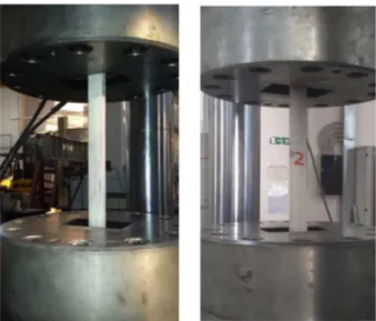
with reference to a case study. The sample configuration considered to
this scope (a double-lap joint made of GFRP parts), is shown in
Figs. 1
and 2
(unit length: mm).
Four adherents can be identified: “1a”, “1b”, “2”, and “3”. The
cross-section is the same for all of them (28 mm × 14 mm). Each adhesive
layer is 1.95 mm thick and is made of an epoxy resin. The mechanical
properties of GFRP and adhesive are listed in
Tables 1 and 2
.
The GFRP adherents were manufactured and provided for free by
ATP-Pultrusion S.r.l. (Angri, Italy) as well as the epoxy resin, provided
for free by Kerakoll S.p.a (Sassuolo, Italy).
As a preliminary goal, two uniaxial tests have been performed on
pure GFRP samples (
Figs. 3 and 4
) (see
Fig. 5
).
The setup includes appropriate metal devices for the anchoring into
the hydraulic jaws of the testing machine.
Both the preliminary tests (two tests) and the main tests (ten tests)
are designed in order to provoke a dominant axial stress state within the
joint. A multi-step procedure is followed as indicated in
Tables 3 and 4
.
In the case of the main tests, strains are monitored by means of 12
uni-axial strain gauges with a grid size of 6.35 mm, characterized by a
maximum strain capacity up to 3% and accuracy equal to 10
−4%
(
Fig. 6
) (see
Fig. 7
).
An appropriate protective gel is used in order to ensure the strain
gauge reliability. As shown in
Fig. 6
, strain gauges are applied at
Fig. 1. Joint configuration (axonometric view).
Fig. 2. Joint configuration (side view). Table 1
Mechanical properties of GFRP (from the manufacturer).
- Value
Young's modulus E≥30000 N/mm2
Thermal expansion coefficient α≤100×10−6K−1
Tensile strength fu≥700N mm/ 2
Ultimate tensile strain εu≥1.50 %
Table 2
Mechanical properties of Kerabuild Eco Epobond (from the manufacturer).
- Value Comments
Young's modulus E≥2000N mm/ 2 –
Thermal expansion coefficient α≤100×10−6K−1 ( 25− °C≤T≤ +60°C)
Bond strength ≥50N mm/ 2 EN 12188 (angle 50°)
≥60N mm/ 2 EN 12188 (angle 60°) ≥70N mm/ 2 EN 12188 (angle 70°)
Fig. 3. Pure GFRP samples (axonometric view).
defined positions lying on the external sides of adherents “2” and “3”.
Four linear variable displacement transducers (LVDTs) are used to
measure the global elongation of the joint. The experimental data are
acquired by means of a hardware/software system consisting of a data
scanner connected to a personal computer. The scanner guarantees an
automatic and modulated data acquisition, as well as a real-time
ad-justment of the data, due to possible loss of the signal.
At a
fixed displacement, the current axial force (T), measured by
means of a load cell, depends on the sti
ffness of the entire system
(GFRP, adhesive interfaces).
Both the preliminary tests and the main tests are carried out at
constant room temperature (18 °C).
The following aspects are investigated:
2.1.1. Via the preliminary axial tests
- the linearity of the response of pure GFRP samples over cycles and
the evaluation of the elastic modulus (to be compared with the
nominal value given by the manufacturer).
2.1.2. Via the main tests
- the elastic sti
ffness of the joint;
- the elastic limit of the joint;
- the interfacial damage stored over cycles;
- the strain evolution within the bonding length;
- the failure load of the joint.
Although the failure load of the joint is not the actual scope of this
study, its value is evenly detected by means of an additional
final step
consisting of a monotone loading process (elongation) up to failure.
The testing equipment is presented in the following
Fig. 8
.
3. Results
The experimental results concern both the constitutive identi
fica-tion of the basic material (GFRP) and the joint behaviour, which is
a
ffected by the interfacial damage.
3.1. Preliminary tests
The experimental results presented in
Tables 5 and 6
are shown in a
sequential order according to the multi-step procedure summarized in
Figs. 9 and 10
. It is worth noting that the subscripts
“0” and “1”
re-spectively indicate the initial point and the end point of the generic
step. The symbol
“
ε
” indicates the axial strain while the symbol “σ” is
for the axial stress. The amount of non-reversible deformation at the
end of the unloading steps (generic step
“b” or “d”) is also presented.
Fig. 5. Preliminary tests on GFRP samples“1” and “2”.Table 3
Multi-step testing procedure (preliminary tests).
Cycles – (*) Target 1, 2, 3 (a) loading DC +0.50 mm (b) unloading FC 0.00 N (c) loading DC −0.50 mm (d) unloading FC 0.00 N 4, 5, 6 (a) loading DC +1.00 mm (b) unloading FC 0.00 N (c) loading DC −1.00 mm (d) unloading FC 0.00 N
(*)DC: displacement control; FC: force control.
Table 4
Multi-step testing procedure (main experiments).
Cycles (*) Target 1, 2, 3 (a) loading DC +1.00 mm (b) unloading FC 0.00 N (c) loading DC 0.00 mm (d) unloading FC 0.00 N Final loading(**) DC + ∞ mm
(*)DC: displacement control; FC: force control;(**)up to failure.
Moreover, the symbol
“E
01” indicates the Young's modulus evaluated
over the generic step by means of a linear
fitting of the experimental
data.
In
Figs. 9 and 10
displacements and axial forces have been
con-verted to non-dimensional quantities with reference to their maximum
values, usually attained at the end of the Step 4a.
For sample
“1”, the value of the Young's modulus (in traction) is
equal to 33084 N/mm
2(average value over cycles 1, 2, and 3) or
30013 N/mm
2(average value over cycles 4, 5, and 6). The values in
compression are, respectively, 37161 N/mm
2(average value over
cy-cles 1, 2, and 3) and 30994 N/mm
2(average value over cycles 4, 5, and
6).
For sample
“2” the value of the Young's modulus (in traction) is
equal to 37093 N/mm
2(average value over cycles 1, 2, and 3) or
37925 N/mm
2(average value over cycles 4, 5, and 6) while the values
in compression are, respectively, 37023 N/mm
2(average value over
cycles 1, 2, and 3) and 37715 N/mm
2(average value over cycles 4, 5,
and 6).
The previous values represent a better identification of the Young
modulus in comparison with the information presented in
Table 1
. This
plays a pivotal role in the evaluation of the mechanical response of the
joint sample.
3.2. Main tests
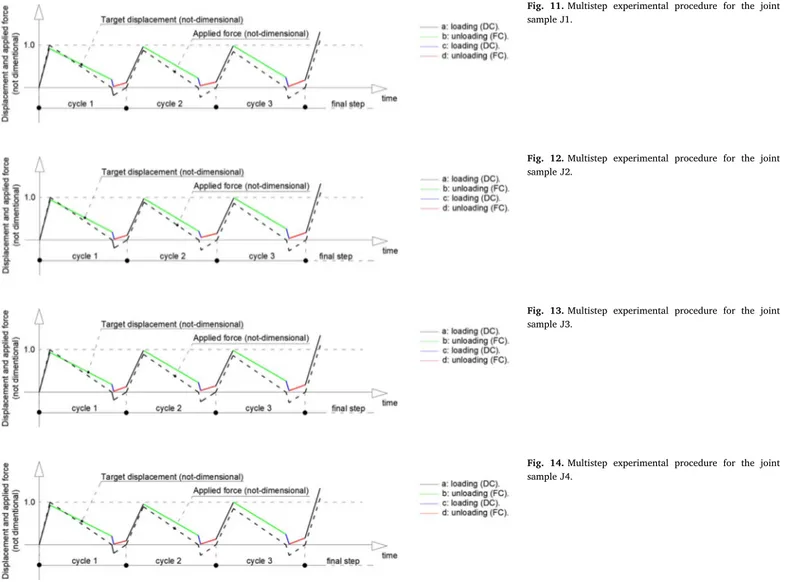
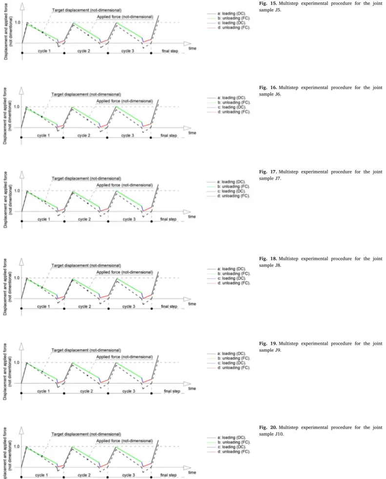
Ten joint samples (J1,
…,J10) are tested according to the multistep
procedure indicated in
Figs. 11
–20
. The experimental results are
pre-sented in
Tables 7–16
.
Similarly to the case of pure GFRP samples, also for the joint
sam-ples the generic step is identi
fied by means of two subscripts, “0” or “1”.
The symbol
“T” is for the axial force while the symbol “ΔL” is for the
axial elongation of the joint, evaluated by means of the LVDT signals. It
is important to remark that the current elongation of the joint is usually
lower than the current target displacement, due to two circumstances:
(i) the free elongation of the end of the sample, behind the adhesion
zone; and (ii) possible sliding within the anchoring devices.
The amount of non-reversible elongation at the end of the unloading
steps is also analyzed. Finally, the symbol
“K
01” indicates the axial
sti
ffness of the joint, evaluated over the generic step by means of a
linear
fitting of the experimental data.
Moreover, the experimental failure loads (T
max) and the
corre-sponding global elongations (
ΔL
max) are summarized in
Table 17
.
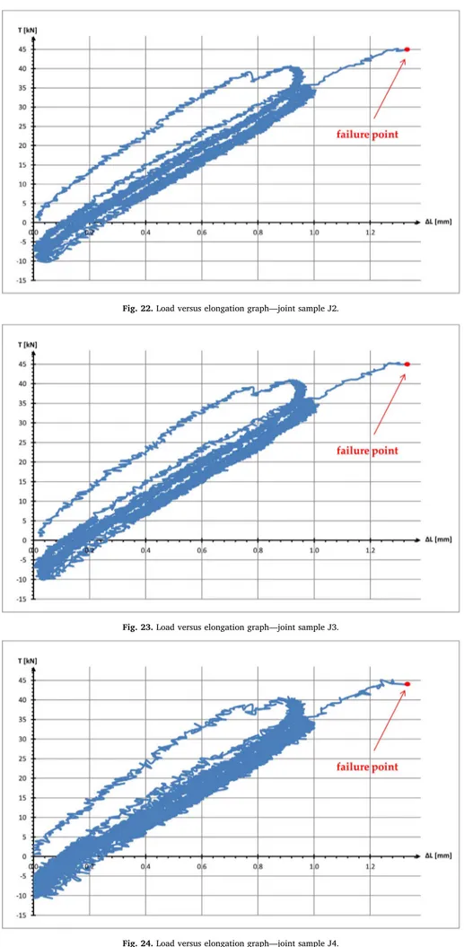
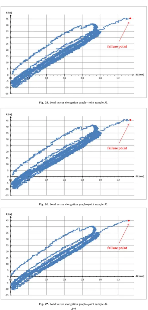
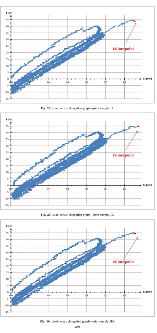
The load versus elongation curves are presented in
Figs. 21
–30
.
Fig. 7. Joint sample“I” (after strain gauges application).Table 5
Preliminary tests (GFRP sample“1”).
Cycle Target εo[%] ε1[%] σo[MPa] σ1[MPa] E01[MPa]
1 loading 1.a DC +0.5 mm 0.000 0.161 0.00 53.14 33642 unloading 1.b FC 0.0 N 0.161 0.006 53.14 0.00 33349 loading 1.c DC −0.5 mm 0.006 −0.161 0.00 −53.49 32763 unloading 1.d FC 0.0 N −0.161 −0.038 −53.49 0.00 41828 2 loading 2.a DC +0.5 mm −0.038 0.161 0.00 65.62 33221 unloading 2.b FC 0.0 N 0.161 −0.030 65.62 0.00 33173 loading 2.c DC −0.5 mm −0.030 −0.161 0.00 −42.74 32821 unloading 2.d FC 0.0 N −0.161 −0.064 −42.74 0.00 41227 3 loading 3.a DC +0.5 mm −0.064 0.162 0.00 72.79 32515 unloading 3.b FC 0.0 N 0.162 −0.055 72.79 0.00 32602 loading 3.c DC −0.5 mm −0.055 −0.161 0.00 −34.32 32542 unloading 3.d FC 0.0 N −0.161 −0.082 −34.32 0.00 41784 4 loading 4.a DC +1.0 mm −0.082 0.321 0.00 119.45 30426 unloading 4.b FC 0.0 N 0.321 −0.006 119.45 0.00 32971 loading 4.c DC −1.0 mm −0.006 −0.323 0.00 −86.32 27121 unloading 4.d FC 0.0 N −0.323 −0.119 −86.32 0.00 38172 5 loading 5.a DC +1.0 mm −0.119 0.322 0.00 115.97 26826 unloading 5.b FC 0.0 N 0.322 −0.005 115.97 0.00 32140 loading 5.c DC −1.0 mm −0.005 −0.323 0.00 −83.12 26262 unloading 5.d FC 0.0 N −0.323 −0.107 −83.12 0.00 35486 6 loading 6.a DC +1.0 mm −0.107 0.323 0.00 109.51 26016 unloading 6.b FC 0.0 N 0.323 0.007 109.51 0.00 31701 loading 6.c DC −1.0 mm 0.007 −0.323 0.00 −82.81 25243 unloading 6.d FC 0.0 N −0.323 −0.098 −82.81 0.00 33678 Table 6
Preliminary tests (GFRP sample“2”).
Cycle Target εo[%] ε1[%] σo[MPa] σ1[MPa] E01[MPa]
1 loading 1.a DC +0.5 mm 0.000 0.162 0.00 54.44 33986 unloading 1.b FC 0.0 N 0.162 0.019 54.44 0.00 36640 loading 1.c DC −0.5 mm 0.019 −0.162 0.00 −62.66 34932 unloading 1.d FC 0.0 N −0.162 −0.004 −62.66 0.00 38586 2 loading 2.a DC +0.5 mm −0.004 0.161 0.00 57.97 35174 unloading 2.b FC 0.0 N 0.161 0.021 57.97 0.00 40150 loading 2.c DC −0.5 mm 0.021 −0.162 0.00 −65.81 36181 unloading 2.d FC 0.0 N −0.162 0.008 −65.81 0.00 37717 3 loading 3.a DC +0.5 mm 0.008 0.161 0.00 54.91 36079 unloading 3.b FC 0.0 N 0.161 0.031 54.91 0.00 40531 loading 3.c DC −0.5 mm 0.031 −0.162 0.00 −70.15 36721 unloading 3.d FC 0.0 N −0.162 0.018 −70.15 0.00 38001 4 loading 4.a DC +1.0 mm 0.018 0.323 0.00 107.01 35550 unloading 4.b FC 0.0 N 0.323 0.074 107.01 0.00 41001 loading 4.c DC −1.0 mm 0.074 −0.328 0.00 −136.69 34713 unloading 4.d FC 0.0 N −0.328 −0.006 −136.69 0.00 40143 5 loading 5.a DC +1.0 mm −0.006 0.323 0.00 112.47 34268 unloading 5.b FC 0.0 N 0.323 0.069 112.47 0.00 40975 loading 5.c DC −1.0 mm 0.069 −0.323 0.00 −137.65 35248 unloading 5.d FC 0.0 N −0.323 −0.007 −137.65 0.00 40376 6 loading 6.a DC +1.0 mm −0.007 0.323 0.00 112.98 34334 unloading 6.b FC 0.0 N 0.323 0.069 112.98 0.00 41424 loading 6.c DC −1.0 mm 0.069 −0.323 0.00 −138.01 35554 unloading 6.d FC 0.0 N −0.323 −0.013 −138.01 0.00 40253
Fig. 9. Multistep experimental procedure for preliminary tests (GFRP sample“1”).
Fig. 10. Multistep experimental procedure for preliminary tests (GFRP sample“2”).
Fig. 11. Multistep experimental procedure for the joint sample J1.
Fig. 12. Multistep experimental procedure for the joint sample J2.
Fig. 13. Multistep experimental procedure for the joint sample J3.
Fig. 14. Multistep experimental procedure for the joint sample J4.
Fig. 15. Multistep experimental procedure for the joint sample J5.
Fig. 16. Multistep experimental procedure for the joint sample J6.
Fig. 17. Multistep experimental procedure for the joint sample J7.
Fig. 18. Multistep experimental procedure for the joint sample J8.
Fig. 19. Multistep experimental procedure for the joint sample J9.
Fig. 20. Multistep experimental procedure for the joint sample J10.
Table 7
Main test—joint sample J1.
Cycle Target To[kN] T1[kN] ΔLo[mm] ΔL1[mm] K01[kN/mm] 1 loading 1.a DC +1.0 mm 0.000 40.552 0.0000 0.9208 50459 unloading 1.b FC 0.0 N 40.552 0.000 0.9208 0.1889 47474 loading 1.c DC 0.0 mm 0.000 −7.465 0.1889 0.0255 48938 unloading 1.d FC 0.0 N −7.465 0.000 0.0255 0.1152 65214 2 loading 2.a DC +1.0 mm 0.000 35.588 0.1152 0.9628 44066 unloading 2.b FC 0.0 N 35.588 0.000 0.9628 0.2203 44359 loading 2.c DC 0.0 mm 0.000 −9.139 0.2203 0.0451 49520 unloading 2.d FC 0.0 N −9.139 0.000 0.0451 0.1331 66079 3 loading 3.a DC +1.0 mm 0.000 34.347 0.1331 0.9832 43610 unloading 3.b FC 0.0 N 34.347 0.000 0.9832 0.2438 43787 loading 3.c DC 0.0 mm 0.000 −10.198 0.2438 0.0267 48033 unloading 3.d FC 0.0 N −10.198 0.000 0.0267 0.1788 60666 loading final DC → +∞ mm 0.000 44.700 0.1788 1.3092 44155 Table 8
Main test—joint sample J2.
Cycle Target To[kN] T1 [kN] ΔLo[mm] ΔL1[mm] K01[kN/mm] 1 loading 1.a DC +1.0 mm 0.000 40.241 0.0000 0.9462 44166 unloading 1.b FC 0.0 N 40.241 0.000 0.9462 0.1855 47174 loading 1.c DC 0.0 mm 0.000 −7.667 0.1855 0.0202 48648 unloading 1.d FC 0.0 N −7.667 0.000 0.0202 0.1112 63426 2 loading 2.a DC +1.0 mm 0.000 35.749 0.1112 0.9733 43950 unloading 2.b FC 0.0 N 35.749 0.000 0.9733 0.2024 44307 loading 2.c DC 0.0 mm 0.000 −9.464 0.2024 0.0618 49014 unloading 2.d FC 0.0 N −9.464 0.000 0.0618 0.1533 63892 3 loading 3.a DC +1.0 mm 0.000 34.682 0.1533 0.9890 43454 unloading 3.b FC 0.0 N 34.682 0.000 0.9890 0.2595 43808 loading 3.c DC 0.0 mm 0.000 −10.243 0.2595 0.0367 49110 unloading 3.d FC 0.0 N −10.243 0.000 0.0367 0.1744 59896 loading final DC → +∞ mm 0.000 44.826 0.1744 1.3228 43935 Table 9
Main test—joint sample J3.
Cycle Target To[kN] T1 [kN] ΔLo[mm] ΔL1[mm] K01[kN/mm] 1 loading 1.a DC +1.0 mm 0.000 40.847 0.0000 0.9364 50599 unloading 1.b FC 0.0 N 40.847 0.000 0.9364 0.1811 46628 loading 1.c DC 0.0 mm 0.000 −7.542 0.1811 0.0214 46883 unloading 1.d FC 0.0 N −7.542 0.000 0.0214 0.1290 62156 2 loading 2.a DC +1.0 mm 0.000 36.299 0.1290 0.9810 44027 unloading 2.b FC 0.0 N 36.299 0.000 0.9810 0.2256 44268 loading 2.c DC 0.0 mm 0.000 −9.071 0.2256 0.0393 48550 unloading 2.d FC 0.0 N −9.071 0.000 0.0393 0.1472 63113 3 loading 3.a DC +1.0 mm 0.000 35.120 0.1472 0.9805 43274 unloading 3.b FC 0.0 N 35.120 0.000 0.9805 0.2634 43911 loading 3.c DC 0.0 mm 0.000 −10.032 0.2634 0.0351 46268 unloading 3.d FC 0.0 N −10.032 0.000 0.0351 0.1733 58584 loading final DC → +∞ mm 0.000 44.912 0.1733 1.3351 42774
Table 10
Main test—joint sample J4.
Cycle Target To[kN] T1 [kN] ΔLo[mm] ΔL1[mm] K01[kN/mm] 1 loading 1.a DC +1.0 mm 0.000 40.343 0.0000 0.9307 50822 unloading 1.b FC 0.0 N 40.343 0.000 0.9307 0.2010 46570 loading 1.c DC 0.0 mm 0.000 −8.048 0.2010 0.0151 45112 unloading 1.d FC 0.0 N −8.048 0.000 0.0151 0.0925 56725 2 loading 2.a DC +1.0 mm 0.000 36.052 0.0925 0.9548 43778 unloading 2.b FC 0.0 N 36.052 0.000 0.9548 0.2188 44151 loading 2.c DC 0.0 mm 0.000 −10.056 0.2188 0.0154 50138 unloading 2.d FC 0.0 N −10.056 0.000 0.0154 0.1330 60009 3 loading 3.a DC +1.0 mm 0.000 34.251 0.1330 0.9999 42683 unloading 3.b FC 0.0 N 34.251 0.000 0.9999 0.2469 43666 loading 3.c DC 0.0 mm 0.000 −10.116 0.2469 0.0145 43632 unloading 3.d FC 0.0 N −10.116 0.000 0.0145 0.1607 55278 loading final DC → +∞ mm 0.000 43.926 0.1607 1.3305 42642 Table 11
Main test—joint sample J5.
Cycle Target To[kN] T1 [kN] ΔLo[mm] ΔL1[mm] K01[kN/mm] 1 loading 1.a DC +1.0 mm 0.000 41.067 0.0000 0.9072 50812 unloading 1.b FC 0.0 N 41.067 0.000 0.9072 0.1730 46886 loading 1.c DC 0.0 mm 0.000 −7.388 0.1730 0.0218 46131 unloading 1.d FC 0.0 N −7.388 0.000 0.0218 0.1236 60677 2 loading 2.a DC +1.0 mm 0.000 36.133 0.1236 0.9798 42883 unloading 2.b FC 0.0 N 36.133 0.000 0.9798 0.2050 44021 loading 2.c DC 0.0 mm 0.000 −8.919 0.2050 0.0299 47021 unloading 2.d FC 0.0 N −8.919 0.000 0.0299 0.1550 61926 3 loading 3.a DC +1.0 mm 0.000 34.944 0.1550 0.9935 42960 unloading 3.b FC 0.0 N 34.944 0.000 0.9935 0.2497 43742 loading 3.c DC 0.0 mm 0.000 −10.213 0.2497 0.0563 49656 unloading 3.d FC 0.0 N −10.213 0.000 0.0563 0.1749 59759 loading final DC → +∞ mm 0.000 45.331 0.1749 1.3366 42819 Table 12
Main test—joint sample J6.
Cycle Target To[kN] T1 [kN] ΔLo[mm] ΔL1[mm] K01[kN/mm] 1 loading 1.a DC +1.0 mm 0.000 40.967 0.0000 0.9085 45178 unloading 1.b FC 0.0 N 40.967 0.000 0.9085 0.1635 46817 loading 1.c DC 0.0 mm 0.000 −7.132 0.1635 0.0284 45761 unloading 1.d FC 0.0 N −7.132 0.000 0.0284 0.1073 62861 2 loading 2.a DC +1.0 mm 0.000 36.115 0.1073 0.9831 44243 unloading 2.b FC 0.0 N 36.115 0.000 0.9831 0.2133 44292 loading 2.c DC 0.0 mm 0.000 −8.351 0.2133 0.0272 44187 unloading 2.d FC 0.0 N −8.351 0.000 0.0272 0.1342 60633 3 loading 3.a DC +1.0 mm 0.000 35.261 0.1342 1.0135 42866 unloading 3.b FC 0.0 N 35.261 0.000 1.0135 0.2511 43717 loading 3.c DC 0.0 mm 0.000 −9.821 0.2511 0.0606 49902 unloading 3.d FC 0.0 N −9.821 0.000 0.0606 0.1707 59332 loading final DC → +∞ mm 0.000 45.962 0.1707 1.3374 42846
Table 13
Main test—joint sample J7.
Cycle Target To[kN] T1 [kN] ΔLo[mm] ΔL1[mm] K01[kN/mm] 1 loading 1.a DC +1.0 mm 0.000 39.235 0.0000 0.9410 50453 unloading 1.b FC 0.0 N 39.235 0.000 0.9410 0.1856 46591 loading 1.c DC 0.0 mm 0.000 −8.291 0.1856 0.0180 47955 unloading 1.d FC 0.0 N −8.291 0.000 0.0180 0.1198 63343 2 loading 2.a DC +1.0 mm 0.000 35.157 0.1199 0.9675 42772 unloading 2.b FC 0.0 N 35.157 0.000 0.9676 0.2215 44136 loading 2.c DC 0.0 mm 0.000 −9.452 0.2216 0.0148 46357 unloading 2.d FC 0.0 N −9.452 0.000 0.0149 0.1387 65389 3 loading 3.a DC +1.0 mm 0.000 33.503 0.1387 0.9924 42331 unloading 3.b FC 0.0 N 33.503 0.000 0.9925 0.2598 43677 loading 3.c DC 0.0 mm 0.000 −10.650 0.2599 0.0161 46483 unloading 3.d FC 0.0 N −10.650 0.000 0.0161 0.2036 59799 loading final DC → +∞ mm 0.000 44.623 0.2036 1.3080 42578 Table 14
Main test—joint sample J8.
Cycle Target To[kN] T1 [kN] ΔLo[mm] ΔL1[mm] K01[kN/mm] 1 loading 1.a DC +1.0 mm 0.000 39.555 0.0000 0.9372 43172 unloading 1.b FC 0.0 N 39.555 0.000 0.9372 0.1829 46577 loading 1.c DC 0.0 mm 0.000 −8.528 0.1830 0.0114 48051 unloading 1.d FC 0.0 N −8.528 0.000 0.0114 0.0969 63095 2 loading 2.a DC +1.0 mm 0.000 35.476 0.0970 0.9532 42705 unloading 2.b FC 0.0 N 35.476 0.000 0.9532 0.2293 44101 loading 2.c DC 0.0 mm 0.000 −10.088 0.2293 0.0414 50392 unloading 2.d FC 0.0 N −10.088 0.000 0.0415 0.1517 65572 3 loading 3.a DC +1.0 mm 0.000 33.106 0.1518 0.9680 41229 unloading 3.b FC 0.0 N 33.106 0.000 0.9681 0.2670 43413 loading 3.c DC 0.0 mm 0.000 −11.269 0.2670 0.0089 46701 unloading 3.d FC 0.0 N −11.269 0.000 0.0089 0.1845 59450 loading final DC → +∞ mm 0.000 43.957 0.1846 1.2990 42495 Table 15
Main test—joint sample J9.
Cycle Target To[kN] T1 [kN] ΔLo[mm] ΔL1[mm] K01[kN/mm] 1 loading 1.a DC +1.0 mm 0.000 40.103 0.0000 0.9624 50661 unloading 1.b FC 0.0 N 40.103 0.000 0.9624 0.2029 46540 loading 1.c DC 0.0 mm 0.000 −8.119 0.2029 0.0128 45953 unloading 1.d FC 0.0 N −8.119 0.000 0.0129 0.1285 59500 2 loading 2.a DC +1.0 mm 0.000 35.356 0.1285 0.9878 43181 unloading 2.b FC 0.0 N 35.356 0.000 0.9878 0.2598 44165 loading 2.c DC 0.0 mm 0.000 −9.413 0.2599 0.0366 42562 unloading 2.d FC 0.0 N −9.413 0.000 0.0367 0.1682 60910 3 loading 3.a DC +1.0 mm 0.000 34.814 0.1683 0.9977 42667 unloading 3.b FC 0.0 N 34.814 0.000 0.9978 0.2639 43744 loading 3.c DC 0.0 mm 0.000 −10.758 0.2640 0.0406 48934 unloading 3.d FC 0.0 N −10.758 0.000 0.0407 0.1951 58405 loading final DC → +∞ mm 0.000 44.504 0.1951 1.3428 42609
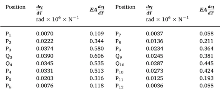
Moreover, the analysis of the strain gauge signals represents the
required veri
fication of the reliability of the experimental tests.
In
Tables 18–27
, the strain gradients (de dT
i/
) attained within the
FRP over the four adhesive interfaces are presented, with
e
ibeing the
strain returned by the electrical gauge placed at the location P
i(
Fig. 31
)
and T the applied axial force. The strain gradients have been averaged
over the loading step
“1a” (cycle 1). Moreover, they are magnified by
×
1
10
6. Four additional positions have been considered (Q
i
, i = 3, 4, 9,
10). They represent relevant cross-sections of the equilibrium scheme
depicted in
Fig. 31
. It is important to underline that the strain gradients
at these locations are evaluated from a linear extrapolation based on the
actual measurements of the neighboring strain gauges. As an example,
the strain at Q
3has been evaluated accounting for the strains attained at
P
1, P
2, and P
3. The last column shows the gradient of the axial force
attained within the external adherents of the joint (adherents
“2” and
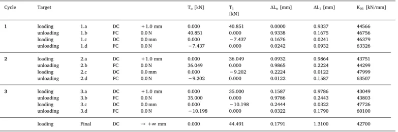
Table 16Main test—joint sample J10.
Cycle Target To[kN] T1 [kN] ΔLo[mm] ΔL1[mm] K01[kN/mm] 1 loading 1.a DC +1.0 mm 0.000 40.851 0.0000 0.9337 44566 unloading 1.b FC 0.0 N 40.851 0.000 0.9338 0.1675 46756 loading 1.c DC 0.0 mm 0.000 −7.437 0.1676 0.0241 46379 unloading 1.d FC 0.0 N −7.437 0.000 0.0242 0.0932 63326 2 loading 2.a DC +1.0 mm 0.000 36.049 0.0932 0.9864 43751 unloading 2.b FC 0.0 N 36.049 0.000 0.9865 0.2224 44299 loading 2.c DC 0.0 mm 0.000 −9.202 0.2224 0.0122 47999 unloading 2.d FC 0.0 N −9.202 0.000 0.0122 0.1587 63507 3 loading 3.a DC +1.0 mm 0.000 35.000 0.1587 0.9786 43049 unloading 3.b FC 0.0 N 35.000 0.000 0.9786 0.2443 43803 loading 3.c DC 0.0 mm 0.000 −10.198 0.2444 0.0322 47726 unloading 3.d FC 0.0 N −10.198 0.000 0.0322 0.1790 60100 loading Final DC → +∞ mm 0.000 44.491 0.1791 1.3100 42700 Table 17
Failure loads and global elongations.
Sample Tmax [kN] ΔLmax[mm] J1 44.700 1.3092 J2 44.826 1.3228 J3 44.912 1.3351 J4 43.926 1.3306 J5 45.330 1.3366 J6 45.962 1.3374 J7 44.622 1.3081 J8 43.957 1.2990 J9 44.500 1.3429 J10 44.491 1.3100
Fig. 22. Load versus elongation graph—joint sample J2.
Fig. 25. Load versus elongation graph—joint sample J5.
Fig. 28. Load versus elongation graph—joint sample J8.
Table 18
Strain and axial force gradients—joint sample J1. Position dei dT rad × 106× N−1 EAdei dT Position dei dT rad × 106× N−1 EAdei dT P1 0.0082 0.128 P7 0.0067 0.103 P2 0.0214 0.332 P8 0.0150 0.233 P3 0.0346 0.537 P9 0.0233 0.362 Q3 0.0361 0.560 Q9 0.0242 0.376 Q4 0.0330 0.513 Q10 0.0271 0.421 P4 0.0320 0.496 P10 0.0259 0.402 P5 0.0221 0.343 P11 0.0182 0.283 P6 0.0123 0.191 P12 0.0038 0.060 Table 19
Strain and axial force gradients—joint sample J2. Position dei dT rad × 106× N−1 EAdei dT Position dei dT rad × 106× N−1 EAdei dT P1 0.0067 0.105 P7 0.0156 0.243 P2 0.0204 0.316 P8 0.0205 0.318 P3 0.0340 0.528 P9 0.0254 0.394 Q3 0.0356 0.552 Q9 0.0259 0.402 Q4 0.0328 0.508 Q10 0.0287 0.446 P4 0.0312 0.483 P10 0.0279 0.433 P5 0.0168 0.261 P11 0.0192 0.297 P6 0.0025 0.039 P12 0.0130 0.202 Table 20
Strain and axial force gradients—joint sample J3. Position dei dT rad × 106× N−1 EAdei dT Position dei dT rad × 106× N−1 EAdei dT P1 0.0085 0.131 P7 0.0011 0.017 P2 0.0223 0.347 P8 0.0124 0.193 P3 0.0362 0.562 P9 0.0238 0.369 Q3 0.0378 0.586 Q9 0.0251 0.389 Q4 0.0340 0.528 Q10 0.0285 0.442 P4 0.0326 0.505 P10 0.0273 0.424 P5 0.0193 0.299 P11 0.0113 0.175 P6 0.0060 0.093 P12 0.0060 0.093 Table 22
Strain and axial force gradients—joint sample J5. Position dei dT rad × 106× N−1 EAdei dT Position dei dT rad × 106× N−1 EAdei dT P1 0.0031 0.049 P7 0.0027 0.042 P2 0.0197 0.305 P8 0.0117 0.181 P3 0.0362 0.562 P9 0.0207 0.321 Q3 0.0380 0.590 Q9 0.0217 0.336 Q4 0.0340 0.528 Q10 0.0259 0.402 P4 0.0325 0.504 P10 0.0247 0.383 P5 0.0186 0.289 P11 0.0090 0.139 P6 0.0047 0.073 P12 0.0027 0.043 Table 23
Strain and axial force gradients—joint sample J6. Position dei dT rad × 106× N−1 EAdei dT Position dei dT rad × 106× N−1 EAdei dT P1 0.0087 0.134 P7 0.0009 0.013 P2 0.0209 0.324 P8 0.0129 0.200 P3 0.0331 0.514 P9 0.0249 0.386 Q3 0.0345 0.535 Q9 0.0262 0.407 Q4 0.0298 0.462 Q10 0.0313 0.486 P4 0.0287 0.446 P10 0.0300 0.465 P5 0.0196 0.304 P11 0.0134 0.207 P6 0.0105 0.163 P12 0.0052 0.080 Table 24
Strain and axial force gradients—joint sample J7. Position dei dT rad × 106× N−1 EAdei dT Position dei dT rad × 106× N−1 EAdei dT P1 0.0102 0.159 P7 0.0034 0.052 P2 0.0224 0.348 P8 0.0142 0.220 P3 0.0346 0.537 P9 0.0250 0.388 Q3 0.0360 0.558 Q9 0.0262 0.406 Q4 0.0347 0.538 Q10 0.0277 0.429 P4 0.0332 0.515 P10 0.0264 0.409 P5 0.0201 0.312 P11 0.0114 0.177 P6 0.0070 0.109 P12 0.0035 0.055 Table 21
Strain and axial force gradients—joint sample J4. Position dei dT rad × 106× N−1 EAdei dT Position dei dT rad × 106× N−1 EAdei dT P1 0.0078 0.121 P7 0.0002 0.004 P2 0.0210 0.325 P8 0.0133 0.206 P3 0.0342 0.530 P9 0.0264 0.409 Q3 0.0356 0.553 Q9 0.0278 0.431 Q4 0.0330 0.512 Q10 0.0301 0.467 P4 0.0317 0.492 P10 0.0290 0.449 P5 0.0199 0.309 P11 0.0153 0.238 P6 0.0081 0.125 P12 0.0081 0.126 Table 25
Strain and axial force gradients—joint sample J8. Position dei dT rad × 106× N−1 EAdei dT Position dei dT rad × 106× N−1 EAdei dT P1 0.0048 0.074 P7 0.0017 0.027 P2 0.0205 0.318 P8 0.0119 0.185 P3 0.0362 0.562 P9 0.0221 0.343 Q3 0.0380 0.589 Q9 0.0232 0.360 Q4 0.0357 0.554 Q10 0.0249 0.387 P4 0.0340 0.527 P10 0.0238 0.369 P5 0.0186 0.288 P11 0.0095 0.147 P6 0.0032 0.050 P12 0.0029 0.044
“3” indicated in
Fig. 2
). They have been evaluated by means of the
following relationship: EA de dT
i/
, with EA denoting the axial stiffness
of the GFRP adherent (EA = 37000 N/mm
2× 28 mm × 14 mm),
esti-mated accounting for the experimental characterization of the Young's
modulus of the GFRP explained in Section
3.1
.
As it is easy to realize, the strain analysis allows the estimation of
the gradient of axial forces N
′ and N″ with respect to the equilibrium
scheme of the joint (
Fig. 31
). It emerges that the global gradient at the
left cross-section Q3
–Q9 (dN'/dT + dN'′/dT) is substantially equal to
the one attained at the right cross-section Q4–Q10 (dN'/dT + dN'′/dT)
for all the joint samples, thus indicating that equilibrium is satisfied
with a quasi-balanced distribution of the axial forces between the
ex-ternal adherents
“2” and “3”. It is important to remark that strain
gauges are applied to the top/bottom sides of the external adherents
and are unable to account for possible shear deformations within the
thickness of the GFRP. This in general, together with experimental
minor errors, may be responsible for the following apparent paradoxes:
′
+
″
≠
N
T
N
T
(a)
d
/d
d
/d
1
′
≠
′
N
T Q
N
T Q
(b)
d
/d
3d
/d
4″
≠
″
N
T Q
N
T Q
(c)
d
/d
9d
/d
10It is worthy of noting that the prediction of the joint behaviour
should account for the interfacial damage due to cyclic loads. A possible
simple approach may be based on a linear model of the joint where a
reduced sti
ffness is implemented. More in detail, for the above
de-scribed case study, this can be established considering the average
va-lues of the stiffness parameter K
01evaluated over the steps 3.a and 3.b,
as in
Table 28
.
The residual sti
ffness of the joint could be assumed from the average
values, provided that an exclusion should occur for data with a
differ-ence more than a certain threshold with respect to the stiffness
corre-sponding to the
final step. For example, if the chosen threshold is fixed
equal to 2%, then all data in
Table 28
could be used for calibrating the
residual stiffness.
4. Conclusions
In this paper, a study dealing with double lap joints made of GFRP
under cyclic loads is conducted. An experimental setup is presented.
This is based on a multistep loading/unloading sequence useful to
in-vestigate the interfacial damage over cycles. It is shown how the
ex-perimental data can be used for estimating, via a simple approach, the
residual stiffness of the joint by means of a cautionary reduction of the
nominal sti
ffness value.
Table 26
Strain and axial force gradients—joint sample J9. Position dei dT rad × 106× N−1 EAdei dT Position dei dT rad × 106× N−1 EAdei dT P1 0.0089 0.138 P7 0.0082 0.127 P2 0.0216 0.335 P8 0.0164 0.255 P3 0.0342 0.531 P9 0.0246 0.382 Q3 0.0356 0.553 Q9 0.0255 0.396 Q4 0.0337 0.522 Q10 0.0276 0.428 P4 0.0322 0.500 P10 0.0264 0.410 P5 0.0193 0.300 P11 0.0131 0.204 P6 0.0064 0.100 P12 0.0057 0.089 Table 27
Strain and axial force gradients—joint sample J10. Position dei dT rad × 106× N−1 EAdei dT Position dei dT rad × 106× N−1 EAdei dT P1 0.0070 0.109 P7 0.0037 0.058 P2 0.0222 0.344 P8 0.0136 0.211 P3 0.0374 0.580 P9 0.0234 0.364 Q3 0.0390 0.606 Q9 0.0245 0.381 Q4 0.0345 0.535 Q10 0.0287 0.445 P4 0.0331 0.513 P10 0.0273 0.424 P5 0.0203 0.316 P11 0.0125 0.193 P6 0.0076 0.118 P12 0.0036 0.055
Fig. 31. Strain gauges locations and equilibrium scheme (unit length: mm).
Table 28
Stiffness values (K01)– unit: N/mm2.
Step J1 J2 J3 J4 J5 J6 J7 J8 J9 J10
3.a (loading) 43610 43454 43274 42683 42960 42866 42331 41229 42667 43049
3.b (unloading) 43787 43808 43911 43666 43742 43717 43677 43413 43744 43803
Average values 43699 43631 43593 43175 43351 43292 43004 42321 43206 43426
Final step values 44155 43935 42774 42642 42819 42846 42578 42495 42609 42700
Acknowledgments
ATP-Pultrusion S.r.l. and Kerakoll S.p.a. companies contributed to
this research providing for free GFRP samples and the epoxy-resin,
spectively. No other grant nor funds there were in support of the
re-search.
Conflicts of interest
The A.T.P. S.r.l. and Kerakoll S.p.a. companies had no role in this
study.
References
[1] Orefice A, Mancusi G, Feo L, Fraternali F. Cohesive interface behaviour and local shear strains in axially loaded composite annular tube. Compos Struct 2017;160:1126–35.
[2] Mancusi G, Orefice A, Feo L, Fraternali F. Structural analysis of adhesive bonding for thick-walled tubular composite profiles. ECCOMAS congress 2016-proceedings of the 7th European congress on computational methods in applied sciences and engineering, vol. 4. 2016. p. 7837–52.
[3] Hasegawa K, Crocombe AD, Coppuck F, Jewell D, Maher S. Characterising bonded joints with a thick andflexible adhesive layer-Part 1: fracture testing and behaviour. Int J Adhes Adhes 2015;63:124–31.
[4] Hasegawa K, Crocombe AD, Coppuck F, Jewell D, Maher S. Characterising bonded joints with a thick andflexible adhesive layer-Part 2: fracture testing and behaviour. Int J Adhes Adhes 2015;63:158–65.
[5] Chaves FJP, Da Silva LFM, De Moura MFSF, Dillard DA, Esteves VHC. Fracture mechanics tests in adhesively bonded joints: a literature review. J Adhes 2014;90:955–92.
[6] Rodríguez RQ, De Paiva WP, Sollero P, Rodrigues MRB, De Albuquerque ÉL. Failure criteria for adhesively bonded joints. Int J Adhes Adhes 2012;37:26–36. [7] Narayanamurthy V, Chen JF, Cairns J. Improved model for interfacial stresses
ac-counting for the effect of shear deformation in plated beams. Int J Adhes Adhes. 2016;64:33–47.
[8] Mancusi G, Ascione F. Performance at collapse of adhesive bonding. Compos Struct 2013;96:256–61.
[9] Li J, Yan Y, Zhang T, Liang Z. Experimental study of adhesively bonded CFRP joints subjected to tensile loads. Int J Adhes Adhes 2015;57:95–104.
[10] Feo L, Mancusi G. Modeling shear deformability of thin-walled composite beams with open cross-section. Mech Res Commun 2010;37:320–5.
[11] Feo L, Mancusi G. The influence of the shear deformations on the local stress state of pultruded composite profiles. Mech Res Commun 2012;47:44–9.
[12] Mancusi G, Feo L. Non-linear pre-buckling Behaviour of shear deformable thin-walled composite beams with open cross-section. Compos B Eng 2013;47:379–90. [13] Mancusi G, Ascione F, Lamberti M. Pre-buckling Behaviour of composite beams: a
mechanical innovative approach. Compos Struct 2014;117:396–410.
[14] Costa I, Barros J. Tensile creep of a structural epoxy adhesive: experimental and analytical characterization. Int J Adhes Adhes 2015;59:115–24.
[15] Puigvert F, Crocombe AD, Gil L. Fatigue and creep analyses of adhesively bonded anchorages for CFRP tendons. Int J Adhes Adhes. 2014;54:143–54.
[16] Mancusi G, Spadea S, Berardi VP. Experimental analysis on the time-dependent bonding of FRP laminates under sustained loads. Compos B Eng 2013;46:116–22. [17] Marante ME, Flórez-López J. Three-Dimensional analysis of reinforced concrete
frames based on lumped damage mechanics. Int J Solids Struct. 2003;40:5109–23. [18] Amorim DLDF, Sergio PB, Proença SPB, Flórez-López J. A model of fracture in re-inforced concrete arches based on lumped damage mechanics. Int J Solids Struct. 2013;50:4070–9.