DOTTORATO DI RICERCA IN GEOFISICA – XXXI CICLO settore concorsuale 4/a4, settore scientifico-disciplinare geo/10
Ambient seismic noise tomography
of the Antarctic continent
Presentata da: Paride Legovini
Supervisore
Prof. Alberto Armigliato
Co-supervisore
Prof. Andrea Morelli
Coordinatrice dottorato
Prof. Nadia Pinardi
List of Figures v
List of Tables ix
Abstract 11
Acknowledgements 15
1 Antarctic Seismology 17
1.1 General notions on Antarctica . . . 17
1.2 Seismicity of the Antarctic plate . . . 25
1.3 Seismography in Antarctica . . . 28
1.4 Field work . . . 33
2 Noise interferometry 45 2.1 Seismic noise . . . 45
2.2 From noise to the Green’s function . . . 47
2.3 The phase cross-correlation . . . 55
2.4 The phase-weighted stack . . . 57
3 Modelling surface waves 63 3.1 Surface waves . . . 63
3.2 Group and phase velocity measurements . . . 71
4 Data retrieval and processing 75 4.1 Introduction . . . 75
4.2 Raw data operations . . . 77
4.3 Preprocessing . . . 81 iii
4.4 Cross-correlation and stacking . . . 82 4.5 Velocity measurements . . . 87 4.6 Convergence measurements . . . 91 4.7 Seasonal variations . . . 95 5 Inversion 99 5.1 Seismic tomography . . . 99 5.2 Tomographic inversion . . . 102
5.3 Velocity maps and profiles . . . 106
6 Conclusions 119
A Hermes: technical documentation 121
1.1 Antarctica overview map. . . 18
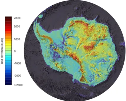
1.2 The Bedmap2 bed elevation model . . . 20
1.3 Antarctic territorial claims . . . 20
1.4 West and East Antarctica . . . 21
1.5 Broad geological structure of Antarctica . . . 23
1.6 Antarctic surface temperature . . . 23
1.7 Countries maintaining antarctic stations . . . 24
1.8 Research stations in the Antarctic . . . 24
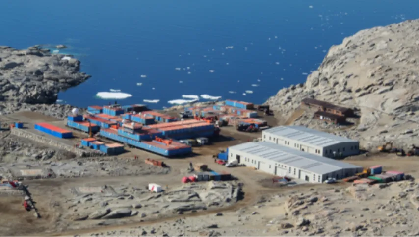
1.9 Aerial view of Mario Zucchelli Station . . . 26
1.10 Aerial view of Concordia Station . . . 26
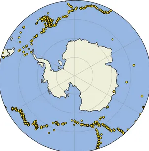
1.11 2000–2010 seismic events with 𝑀W≥ 6 south of 50° S . . . . 27
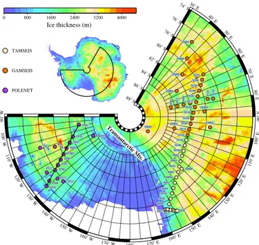
1.12 Seismic arrays in Antarctica . . . 30
1.13 The Terra Nova Bay observatory . . . 31
1.14 The Concordia observatory . . . 33
1.15 The Starr Nunatak station . . . 34
1.16 The 1 January 2016 peri-Antarctic earthquake . . . 35
1.17 The TNV new acquisition system . . . 36
1.18 TNV: data acquisition diagram . . . 39
1.19 TNV: power system diagram. . . 40
1.20 Diagram of the Hermes system . . . 43
2.1 One day of seismic record . . . 46
2.2 PSD for QSPA between 2007 and 2012 . . . 48
2.3 A diffuse noise field . . . 52
2.4 Seismic interferometry: principle . . . 52
2.5 An ideal noise cross-correlation . . . 53 v
2.6 Classic seismic interferometry workflow . . . 54
2.7 A stack of cross-correlations . . . 55
2.8 How the PCC behaves differently . . . 58
2.9 PCC+PWS seismic interferometry workflow . . . 60
2.10 Comparison between classic techniques and PCC/PWS . . . 61
3.1 Arrival of body and surface waves . . . 64
3.2 Velocity of seismic waves in the Earth versus depth . . . 66
3.3 PREM’s main parameters . . . 68
3.4 PREM dispersion curves . . . 69
3.5 PREM sensitivity kernels . . . 69
3.6 Sensitivity kernels for Antarctica . . . 70
3.7 Sample FTAN diagrams . . . 73
4.1 Map of the seismic stations in Antarctica. . . 79
4.2 Station pairs in Antarctica . . . 80
4.3 Cross correlation: AU.MAW G.DRV . . . 84
4.4 Cross correlation: AU.MAW IU.SBA . . . 84
4.5 Cross correlation: G.CCD.10 IU.QSPA . . . 84
4.6 Cross correlation: G.DRV IU.CASY . . . 85
4.7 Cross correlation: G.DRV IU.QSPA . . . 85
4.8 Cross correlation: G.DRV IU.SBA . . . 85
4.9 Cross correlation: GE.SNAA IU.CASY . . . 86
4.10 Cross correlation: GE.SNAA IU.SBA . . . 86
4.11 Cross correlation: IU.QSPA IU.SBA . . . 86
4.12 Dispersion curve for AU.MAW G.DRV . . . 88
4.13 Dispersion curve for G.DRV IU.CASY . . . 88
4.14 Dispersion curve for G.DRV IU.QSPA . . . 88
4.15 Dispersion curve for G.DRV IU.SBA . . . 89
4.16 Dispersion curve for IU.QSPA IU.SBA . . . 89
4.17 FTAN diagram with spectral notches . . . 91
4.18 Convergence plot: G.CCD–GE.SNAA . . . 92
4.19 Convergence plot: G.CCD–AU.MAW . . . 93
4.20 Actual ray coverage . . . 94
4.22 Convergence using summer days . . . 96
4.23 Convergence using winter days . . . 97
5.1 Velocity measurements binning (full) . . . 104
5.2 Velocity measurements binning (clean) . . . 104
5.3 Cubed sphere used for the inversion . . . 106
5.4 Raw model: rays for 𝑇 = 30 s . . . 109
5.5 Raw model: rays for 𝑇 = 80 s. . . 110
5.6 Rayleigh waves velocity model (𝑇 = 30 s) . . . 111
5.7 Rayleigh waves velocity model (𝑇 = 80 s) . . . 112
5.8 Velocity measurements binning (W. Antarctica) . . . 114
5.9 Velocity measurements binning (E. Antarctica) . . . 114
5.10 Avg. dispersion curves for W. and E. Antarctica. . . 115
5.11 Avg. dispersion curves for W. and E. Antarctica (slowness) . 115 5.12 1D 𝑣Sprofiles . . . 116
1.1 Quanterra Q330HR specifications . . . 31
1.2 TNV data QA: reference events . . . 36
1.3 Centering of the TNV instruments . . . 38
3.1 Ten entries of the PREM model . . . 68
4.1 Intel Xeon E5-4607 v2 specs . . . 76
4.2 Number of stations per year . . . 79
4.3 Coords for the stations of figures 4.3 to 4.11 . . . 83
The lithosphere of Antarctica reacts to both the stress variations due to the dynamics of the mantle and the variation of the glacial load due to changes in climate. These two factors, active at different spatial and temporal scales, act on the dynamics of the glacial mass, on the evolution of the continent’s topography and on the seismicity of the Antarctic plate. The knowledge of these interactions is still scarce, but the need for a better comprehension of the processes that involve interactions between climate and the geosphere is increasingly clear.
The main aim of this work is to improve on the current knowledge of the three dimensional structure of the Antarctic lithosphere producing a new continental-scale tomographic model. The knowledge of spatial variations in lithospheric thickness is recognized as a necessity to build a reliable glacial isostatic adjustment model for Antarctica (Nield et al.2018). Seismic tomog-raphy studies of Antarctica already exist but, to the best of my knowledge, they are based on earthquake data and their resolution is limited by the fact that seismic networks on the continent are very scarce and often made by temporary stations installed on the ice sheet, whose quality is not on par with that of permanent seismic stations installed on rock. There is ample room for improvement.
The classic data source for tomographic studies is a set of seismic sig-nals produced by earthquakes. In this work I use a different technique: the information on the elastic properties of lithosphere is extracted by cross-correlating the continuous background vibrations (often referred to as “am-bient seismic noise”) recorded in different locations. This approach is pre-sented inchapter 2and has some advantages with respect to more classic earthquake-based studies. The possibility to perform tomography without
earthquakes is especially valuable in Antarctica, considered its very low seis-mic activity. Besides, the correlation of signal recorded by a pair of stations brings information on the structure comprised between the two stations, giving then optimal sensitivity to continental structure – as opposed to paths from earthquakes, mostly on ocean ridges, that mix oceanic and continental structure. Interferometric techniques have shown unquestioned ability to map crustal structure using microseismic data, but also capacity to image mantle structure using the long-period seismic hum.
Instead of a the classic cross-correlation, this work uses the phase cross
correlation technique, which appears to be more robust than the classic one
in our use case, where input data is often not very clean. Signal phases are used even to improve the correlogram stacks, by weighting the stack samples according to the correlograms’ instantaneous coherence.
I also contributed to the maintenance and development of the seismic observational infrastructure in Antarctica. This thesis then also recaps the activities I carried out during my participation to the 31st campaign of the Italian National Antarctic Research Program (PNRA), to which I participated during the PhD course. These activities did in part follow up to what was my job during the 10th winter campaign at the Concordia research station, which saw me on the ice for the entire year 2014.
The present work is organized as follows. Chapter 1is an overview of the geography, geology and seismicity of Antarctica. Within this chapter,
section 1.3explains how seismic stations are installed on the continent and what are the difficulties and peculiarities of these deployments. This sec-tion also accounts for my activities on the field. Chapter 2treats ambient seismic noise in general and how useful information is extracted from it by cross-correlation and stacking. The chapter introduces the correlation and stacking techniques used in this work: the phase cross-correlation and the phase weighted stack. Chapter 3 is an overview on surface waves and on how they are modelled to gather useful information to later construct a seismic tomography.Chapter 4is more technical, concentrating on the data retrieval and actual processing, and on the difficulties encountered during the analysis. Finally,chapter 5is about the inversion, with an introduction to the inverse problem, a description on the parametrization used in this
study and finally some surface wave velocity maps.Chapter 6draws some conclusions followed by two appendices with additional material.
The phase cross-correlation, and the phase-weighted stacking technique, showed clear advantages — with respect to the conventional linear cross-correlation and stack — in dealing data of heterogeneous quality, as in this case. However, the phase-weighted stack in many cases did not perform optimally, so I had to use a hybrid linear/phase-weighted stacking technique. The preliminary linear stack somehow pre-conditions the signal, letting some coherence grow so that it is then optimally exploited by the later phase weighted stage. Rayleigh-wave dispersion curves could thus be obtained (through automatic frequency-time analysis) from 20 s to 180 s, with the best-observed period interval between 30 s and 80 s. I best-observed some seasonality effects in several, but not all, station pairs, where winter data are faster to converge to a stable Rayleigh wave dispersion curve, than summer data. The reason for this behavior is not completely clear, but it should have to do with better conditions (more coherent ocean-generated microseismic noise, less contamination from local atmospheric-induced disturbance). Performance of observatory-grade seismic installation was obviously more reliable than capacity of temporary stations, particularly so at longer period. This was of course expected. Temporary stations, however, showed generally good performance. Field experiments can also provide very usable data.
I inverted dispersion measurements for maps of Rayleigh group velocity at different periods. Shorter-period maps carry resemblance of crustal and uppermost mantle structure. In Antarctica, the 30 s Rayleigh wave group velocity map shows lower velocities in East Antarctica, and higher velocities in West Antarctica, coherently with expectations related to a thicker cratonic crust in the East, and thinner extending crust in the West. Deeper sensitivity of longer periods make the color pattern switch for the 80 s map, sensing the upper mantle and consequently higher velocity at the cold roots of cratonic East Antarctica and lower velocity in the tectonically active West. So far, the maps I have produced rely entirely on my own measurements. A for-ward extension will formally include additional information resulting from previous studies, as a priori information in the Bayesian inverse formalism.
I would like to thank my advisor Andrea Morelli for his guidance during the last three years: I have learned a lot and I owe it mostly to him. I would also like to thank Alberto Armigliato for his feedback and support during the development of my work and the writing of this thesis: it has been of great importance.
Thanks to Martin Schimmel, Sergi Ventosa and to all the Barcelona group: the discussions we had during my stay at ICTJA have been an invaluable source of ideas and scientific insight.
Thanks to Peter Danecek and Alberto Delladio for giving me the oppor-tunity to participate to the 31st PNRA expedition: working on the field in such a challenging environment has been an extraordinary experience I will never forget.
Antarctic Seismology
1.1
General notions on Antarctica
Geography
Located in the Earth’s southern hemisphere, the Antarctic continent is cen-tered around the South Pole and largely south of the Antarctic Circle, running at about 66°33′south of the Equator. It has an area of more than 14 × 106km2 and is washed by the Southern (or Antarctic) Ocean, which is the southern part of the Pacific, Atlantic, and Indian Oceans (Drewry1983). About 98% of the continent is covered by the Antarctic ice sheet, the world’s largest ice sheet. Its average thickness is of 1.6 km, peaking at 4.8 km, and it is so mas-sive that it has depressed the continental bedrock below sea level (Fretwell et al.2013). The coastline measures about 18 × 103km and is characterized by the presence of ice shelves1, floating ice and other ice formations (Drewry
1983). A general map of the continent is shown infigure 1.1.
A standard gridded map of the surface elevation, ice-thickness and of the the sea floor and subglacial bed elevation of the Antarctic has been produced by the British Antarctic Survey and is known as Bedmap2 (Fretwell et al.
2013). The model incorporates over 25 million measurements from different geophysical and cartographic sources. A preview of the model is shown in
figure 1.2. In September 2018, the National Geospatial–Intelligence Agency (NGA) released the Reference Elevation Model of Antarctica (REMA): a
1. An ice shelf is a floating platform of ice that forms where a glacier or ice sheet flows down to a coastline onto the ocean surface.
2000 3000 4000 0 1000 Km 2000 0 200 400 600 800 1000 Miles 60°S 70°S 80°S 90°E 180°
90°W South PoleAmundsen-Scott (USA)
T ra n s a n tar c t i c M ou n ta in s South Shetland Is Anvers I. Adelaide I. South Orkney Is Alexander I. Peter I Øy Balleny Is GR AH AM LAN D ELLSWORTH LAND MARIE BYRD LAND Vinson Massif 4892m Mtns E llsworth Executive Committee Range Whitmore Mtns s n t M Prince haCrles Thiel Mtns Shackleton Range Thorshav nheine eime h n l u b m i F P ensa cola M tns Berkner Island PAL MER LAN D VIC TOR IA LAN D OATES LAND Mt Erebus COATS LAND DRONNING MAUD LAND ENDERBY LAND KEMP LAND MACROBERTSON PRINCESS ELIZABETH LAND WILHELM II LAND QUEEN MARY LAND WILKES LAND TERRE ADÉLIE GEORGE V LAND LAND Scott Mtns A N TAR CTIC PENINS ULA Rothera (UK) Palmer (USA) Halley (UK) McMurdo (USA) Subglacial Lake Vostok ROSS ICE SHELF A B B O T IC E S H ELF AMERY ICE SHELF SHACKLETON ICE SHELF G E TZ ICE SHELF R O S S S E A A MU NDS E N S E A Dome Argus Dome Fuji (Valkyrie) Dome Circe
Dumont d’U rville S ea Davis S ea P rydz B ay B E L L I NG S HA U S E N S E A WE DDE L L S E A S O U T H E R N O C E A N S O U T H E R N O C E A N K O Å N H V I G I N H O A K V RONNE ICE SHELF FILCHNER ICE SHELF BRUNT ICE SHELF ISEN L U B M I F LARSEN ICE SHELF E A S T A NTA R C T I C A WE S T
A NTA R C T I C A QueenMaud
Mtns Queen Alexandra Range Queen Elizabeth Range Signy (UK) QUEEN ELIZABETH LAND
Figure 1.1 Antarctica overview map showing the main geographic features of the
continent with their names (USGS2018). Dome Circe, Dome Argus and Dome Fuji are also respectively known as Dome C, Dome A and Dome F.
high resolution (8 m) terrain map of nearly the entire continent (Howat et al.
2018).
Seven countries have the partially overlapping territorial claims on part of Antarctica shown infigure 1.3: Argentina, Australia, Chile, France, New Zealand, Norway and the United Kingdom. The validity of these claims is not universally recognized (Division2018). The United States and Russia (formerly as the Soviet Union) reserved the right to make claims in the fu-ture. The international relations with respect to Antarctica are regulated by the Antarctic Treaty. The treaty entered into force in 1961 as a peace-keeping effort and currently has been signed by 53 countries. The treaty sets aside Antarctica as a scientific reserve, establishes freedom of scientific investigation and bans military activity on the continent.
Geological structure
Antarctica is roughly divided in two by Transantarctic Mountains, a moun-tain range of uplifted sedimentary rock which extends across the continent from the north-easternmost peninsula in Victoria Land to Coats Land ( fig-ure 1.1). The two halves are conventionally called West Antarctica and East Antarctica and approximately correspond to the eastern and western hemi-spheres relative to the Greenwich meridian. East Antarctica is larger and includes both the South magnetic pole and geographic South Pole. This division is shown schematically infigure 1.4.
Geologically, West Antarctica closely resembles the Andes of South Amer-ica (Stonehouse2002). The Antarctic Peninsula was formed by uplift and metamorphism of sea-bed sediments during the late Paleozoic and the early Mesozoic eras. This sediment uplift was accompanied by igneous intrusions and volcanism. The only anomalous area of West Antarctica is the Ellsworth Mountains region (figure 1.1), where the stratigraphy is more similar to the eastern part of the continent (Stonehouse2002).
East Antarctica is geologically very old, dating from the Precambrian2, with some rocks formed more than 3 billion years ago. It is composed of a metamorphic and igneous platform which is the basis of the East Antarctic
2. The earliest part of Earth’s history, spanning from the formation of Earth about 4.6 billion years ago to the beginning of the Cambrian Period, about 541 million years ago.
Figure 1.2 The Bedmap2 bed elevation model (Fretwell et al.2013). Chile UK Argentina Norway Australia Australia France New Zealand Marie Byrd Land
Norway (Brazil)
Figure 1.3 Antarctic territorial claims (Division2018). The countries with
terri-torial claims (Argentina, Australia, Chile, France, New Zealand, Norway and the United Kingdom) are all signatories of the Antarctic Treaty. The Marie Byrd Land territory is unclaimed.
Figure 1.4 The Transantarctic Mountains range conventionally divides the con-tinent in two halves: West Antarctica and East Antarctica (modified from Harley
2011). The two halves roughly correspond to the eastern and western hemispheres relative to the Greenwich.
Shield or Antarctic Craton: the old and stable part of the lithosphere that covers the majority of the continent (Drewry1976).
Climate
Antarctica has the coldest climate on Earth. Temperatures reach a minimum of between −80∘C and −89.2∘C in the interior in winter and a maximum of between 5∘C and 15∘C near the coast in summer (Chapman and Walsh
2007). The coldest air temperature ever recorded on Earth was −89.2∘C at the then Soviet Vostok Station (East Antarctica) in July 1983 (Turner et al.
2009). A map of the average surface temperature of Antarctica in winter and summer is shown infigure 1.6.
East Antarctica is colder than its western counterpart because of its higher elevation. Weather fronts rarely penetrate far into the continent, leaving the centre cold and dry. Antarctica is in fact a cold desert, with a snowfall equivalent to 150 mm of water each year (BAS2018). The edge of the continent is often interested by very strong katabatic winds coming from the plateau, while in the interior wind speeds are typically moderate (Parish and Bromwich1991).
Research facilities
As of October 2018 a total of 30 countries maintain permanent research sta-tions in Antarctica. Some of these stasta-tions are staffed year-round, while others operate only during the austral summer (COMNAP2018). The pop-ulation of people performing and supporting scientific research on the conti-nent and nearby islands varies from approximately 4000 during summer to 1000 during winter.Figure 1.7shows the countries that currently maintain at least one permanent research facility in Antarctica, whilefigure 1.8is a map of the permanent facilities.
Italy maintains two permanent research stations: Mario Zucchelli Station (MZS) and Concordia. The stations are run by the National Antarctic Re-search Program (Programma Nazionale di Ricerche in Antartide, PNRA) with their logistics is managed by the National Agency for New Technologies, Energy and Sustainable Economic Development (Agenzia nazionale per le
Figure 1.5 A coarse geological subdivision of Antarctica into three geological regions: the old and stable East Antarctic Shield, the generally younger West Antarc-tic domain, and the Trans-AntarcAntarc-tic domain, along the TransantarcAntarc-tic Mountains (modified from Harley2011).
Figure 1.6 Near surface (1.5 m) temperature of Antarctica in winter and summer
from European Centre for Medium-Range Weather Forecasts (ECMWF) 40 year reanalyses, for the period 1979-2001 (Credit: W. M. Connolley).
Figure 1.7 Countries that maintain at least one permanent research station in Antarctica (COMNAP2018).
Figure 1.8 The permanent research stations in Antarctica (COMNAP2018, credit:
nuove tecnologie, l’energia e lo sviluppo economico sostenibile, ENEA). Mario
Zucchelli Station (figure 1.9) was created in 1985 and is located at Terra Nova Bay, at the coast of Victoria Land, and is staffed only during the austral summer, between October and February. Concordia Station (figure 1.10) is jointly operated by PNRA and the French polar institute Paul-Émile Victor (IPEV), is staffed year-round since 2005 and is located at Dome C, on the East Antarctic plateau, at 3233 m above sea level. Concordia is the third perma-nent, all-year research station on the Antarctic Plateau, the other two being Vostok Station (Russian, formerly Soviet), located near the geomagnetic South pole, in inland Princess Elizabeth Land, and the Amundsen–Scott South Pole Station (USA) located at the geographic South Pole.
1.2
Seismicity of the Antarctic plate
Seismic activity
The Antarctic continent has a number of unique features, one of these is its tectonic setting: its margins are almost everywhere divergent, with only a small fraction of convergent or transformed margins. One consequence of this fact is that the seismicity of the Antarctic plate is quite low when compared with other continental plates. This scarce seismic activity was largely unknown up to a few decades ago due to the lack of instrumentation deployed on the continent. It is noteworthy that the first confirmed earth-quake in continental Antarctica has been recorded in 1985 (Adams, Hughes, and Zhang1985).
A map of the seismic events occurred below 50° S between year 2000 and 2010 and with 𝑀W≥ 6 is shown infigure 1.11. From this figure it is imme-diately evident how the seismic activity is concentrated on the boundaries of the continental plate. The highest magnitudes determined for Antarctic continental intraplate earthquakes are approximately 𝑀W= 4.5, with only a small minority reaching 𝑀W≥ 5.0 (Reading2007). The following outline of the seismicity of Antarctica is best read while keeping figure 1.1 as a reference.
The most seismically active region in continental Antarctica is the region of the Transantarctic Mountains, which forms a belt of larger earthquakes.
Figure 1.9 Aerial view of Mario Zucchelli Station (Terra Nova Bay, along the coast of Victoria Land). The station is staffed only during the austral summer and is operative since 1985.
Figure 1.10 Aerial view of Concordia Station (Dome C, East Antarctic plateau).
The station is staffed year-round since 2005. The picture has been taken installing a camera on a weather balloon.
Figure 1.11 Map of 𝑀W≥ 6 seismic events happened south of 50° S between 2000
and 2010 (USGS data).
Events occurring along the Ross Sea margin through Victoria Land are recorded relatively frequently and microseismicity clusters are known to be associated with the activity of some major glaciers. Isolated events occurred in the regions of Lake Vostok and Dome F, in the East Antarctic. Seismicity in the Weddell Sea has been confirmed by records from an array located near the German Neumayer station on the Dronning Maud Land coast. Recorded earthquakes in the northern part of the peninsula are associated with subduction in the Bransfield Strait (between the South Shetland Islands and the Antarctic Peninsula), while a few are located on the continental rise in the southern Pacific Bellingshausen Sea. In East Antarctica seismic events are clustered along the coast, in the region of Adélie Land. Seismic events are also observed further along the coast of Wilkes Land and offshore of Enderby Land (Kanao2014; Reading2007).
Away from the continental area, the intraplate region northwest of the Balleny Islands (north of Victoria Land) has a very high seismicity, as can be expected given its location close to the plate boundaries that form the junction between the Pacific, Australian, and Antarctic plates. Intraplate seismicity is also observed between the Australian–Antarctic Ridge and the Antarctic continent (Kanao2014; Reading2007). Scattered groups of
intraplate earthquakes occur on the Kerguelen Plateau, in the southern Indian Ocean, while the Crozet Islands and the Prince Edward Islands are very quiet (Reading2007).
1.3
Seismography in Antarctica
Seismic stations
Antarctica represents one of the most extreme and exceptional environments on Earth. It is the most remote continent and in terms of logistics probably the most challenging region to reach, in particular when considering locations in the interior of the continent. As a consequence, the availability of scientific data is rather scarce and the density of instrumental observation points is low. This makes any geophysical observation extremely valuable. At the same time these environmental conditions and practical constraints require special approaches and operational practice.
Seismic instrumentation of Antarctica was a priority for the International Geophysical year (IGY) in 1957 (Hatherton and Evison1962; Lander1959). A total of twelve stations were installed, several becoming permanent in 1963 with the installation of the World Wide Standard Seismographic Network (WWSSN) (Lander1959; Okal1981). Even with the limited station coverage of IGY six events were located south of 65° and twenty were located south of 55° (Lander1959). Before 1963 the earthquake detection threshold was approximately 𝑀W = 6, with the improved WWSSN coverage the detection threshold dropped to approximately 𝑀W= 4.9 (Okal1981).
It is only since the late 1990s that larger scale deployments of temporary stations have become feasible with the advent of more cost efficient, high quality equipment along with increased logistical support. These deploy-ments have typically been very localized, often only covering several hundred square kilometers. As equipment evolved array size also improved. The Transantarctic Seismic Experiment (TAMESIS, Anandakrishnan and Wiens
2000) array, operating during the austral summers of 2000–2003, crossed the Transantarctic Mountains and extended into East Antarctic. The Gam-burtsev Mountains Seismic Experiment (GAMSEIS, Wiens and Nyblade
Gamburt-sev Subglacial Mountains, in East Antarctica, just underneath the Dome A. The Polar Earth Observing Network (POLENET, Wiens and Nyblade2007b), started in 2007 and still operative, has seismic stations deployed across West Antarctica. The locations of these arrays are shown infigure 1.12.
The stations that are part of these temporary seismic arrays complement a smaller number of permanent, observatory grade stations. The difference between the two is on all levels, from the choice of the instruments to the installation site, which is an extremely important factor in the overall data quality. An observatory grade station is visible in figure 1.13, note how the seismometers are installed on a concrete block built within a granite cave. On the contraryfigure 1.15shows a temporary deployment where the instrument is merely protected by some rocks.
The Italian National Institute for Geophysics and Volcanology (INGV) maintains two permanent seismic observatories in Antarctica, installed in the premises of the Italian permanent research stations. Moreover, the in-stitute maintains a semi-permanent station at Starr Nunatak and a number of temporary stations. The stations are part of the MedNet network (INGV
1990).
The Terra Nova Bay observatory
The Terra Nova Bay seismological observatory (station code TNV, 74.70° S 164.12° E) is based at the Mario Zucchelli Station. The first seismological experiments started shortly after the establishment of the Italian scientific station at Terra Nova Bay and led in 1988–1989 to the construction of the permanent seismological observatory, located in an artificial cave dug in granite about 2 km away from the research station and equipped with a set of Streckeisen STS-1/VBB (very broadband) seismometers. With a low frequency corner of the response located at 360 s, the STS-1 is widely re-garded as one of the best instruments available for seismological research for long and very long period studies. The entrance of the cave and the instrumentation are pictured infigure 1.13.
In the current setup the station has two separate and almost independent acquisition chains, one with the original Streckeisen STS-1 sensors, the other with a Streckeisen STS-2 sensor (another observatory-grade instrument, this
Figure 1.12 Locations of the three main seismic arrays in Antarctica: TAMSEIS, GAMSEIS, and POLENET (modified from Yan et al.2018).
one with a low frequency corner of the response located at 120 s). Experi-ence shown that the adverse environmental conditions and the unmanned operation during Antarctic winter requires significant level of redundancy for the acquisitions systems. The current setup features several acquisition and data storage systems both at the cave and in the base. More details will be given insection 1.4.
Regular maintenance is performed yearly along with the recovery of the recorded data. In the recent years the observatory’s acquisition system has been upgraded with modern Quanterra Q330HR digitizers (table 1.1
reports the digitizer’s specifications) and new rugged servers (ALPHA2000 PrioComP) at the cave.
There are plans to bring further improvements on the redundancy and the site infrastructure, in particular regarding power supply, networking and cabling. The ageing STS-1 sensors are increasingly difficult to maintain and opportunities to replace them are being explored.
Figure 1.13 The entrance of the Terra Nova Bay seismic observatory artificial cave and its instrumentation during the evacuation of the STS-1 vacuum chambers.
Main Channels 3 26 bit and 3 24 bit channels
Aux channels 4/8 DI/SE 16 bit 1 sps. Full range 50 V Dynamic range 144 dB to 145 dB wireband rms typical HR Channels 0.02 Hz to 20 Hz 147 dB to 158 dB Gain Selectable per channel: 1 to 20 Filtering Linear or Minimum Phase FIR Sample rates 1 sps to 200 sps
Time base Precision TCXO, phase-locked GPS
The Concordia observatory
The Concordia observatory (station code CCD, 75.11° S 123.31° E, Dome C, East Antarctic Plateau) is jointly operated by INGV and the École et
observa-toire des sciences de la terre (EOST) of Strasbourg, France. The first
seismologi-cal experiments started already before the opening of the permanent base in 2001. In 2005 a permanent observatory was established in an artificial cavity constructed with shipping containers at approximately 12 m of depth. Two independent sensors and acquisition chains are currently operated at the observatory, one equipped with a Streckeisen STS-2 (figure 1.14), the other with a Nanometrics Trillium T240 sensor. The temperature in the cave is very stable at about −55∘C, but the STS-2 is heated to about −30∘C to keep it within its operational limits.
Both chains were recently upgraded with modern Quanterra Q330S digitizers and rugged ALPHA2000 PrioComP servers installed in the seis-mology shelter (hut). Moreover a real-time data transmission to France and a near-realtime data transmission to Italy were recently established. Regular maintenance and recovery of all the recorded data is performed each year.
The observatory is currently undergoing a major upgrade due to the lim-ited lifetime of the subsurface cavity and installations. This upgrade foresees the installation of a post-hole seismic sensor in a borehole approximately 130 m deep. The seismology shelter which in the meantime has been com-pletely covered by snow drift will be replaced by a new wooden shelter on stilt. Currently tests are being carried out with the temporary installation of a near surface Nanometrics Trillium T240 sensor and a Nanometrics Trillium T120 Posthole. During the 2018–2019 summer campaign the drilling and casing of the borehole will be carried out along with the construction of a new shelter for the instrumentation.
The Starr Nunatak station
Figure 1.15shows the semi-permanent autonomous seismic station at Starr Nunatak3at a distance of approximately 150 km from Mario Zucchelli station
and was first installed in the framework of a temporary network in 2003. Later
3. A nunatak is an rocky peak not covered with snow or ice which raises within or at the boundary of a glacier, ice field or polar ice cap.
Figure 1.14 The Streckeisen STS-2 seismometer, part of one of the two acquisition chains of the Concordia seismic observatory (CCD). The sensors are installed at a depth of about 12 m, in a niche dug in snow. The ambient temperature is quite stable at about −55∘C, but the sensor is heated to −30∘C.
its operation continued on a semi-permanent basis and with surprisingly good reliability. This station is powered by solar panels and hibernates during Antarctic winter.
Regular visits to Starr Nunatak are performed in order to retrieve the locally recorded data and perform maintenance operations. For the future we strive to upgrade the station with modern instrumentation and to enable permanent and fully continuos operation.
1.4
Field work
During the PhD course I participated to the 31st expedition of the Italian National Antarctic Research Program (PNRA) to work on the Mario Zuc-chelli and Concordia seismic observatories. This section summarizes the field activities done during the campaign; more details are available in the yearly expedition reports compiled by PNRA (PNRA2015a,b,2016). The data retrieved during the expedition became part of the dataset that had been used in the work that follows in the next chapters.
Figure 1.15 The semi-permanent Starr Nunatak seismic station, about 150 km away from Mario Zucchelli station. Starr Nunatak marks the north side of the mouth of Harbord Glacier, on the coast of Victoria Land. The station operates on solar panels and batteries.
Activities at MZS
Some important interventions were to be done on the Terra Nova Bay ob-servatory on this expedition. This was due the end of the service life of some instruments, and due to some malfunctions that occurred during the austral winter of 2015. Before the beginning of the expedition the state of the instruments was largely unknown, as the mentioned faults interfered with the possibility to remotely control the instruments. The planned inter-ventions, in addition to the ordinary maintenance of the observatory, were the following:
• Replacement of a faulty Quanterra Q4120 digitizer with a newer Quan-terra Q330HR;
• Installation of a new acquisition server;
• Check-up and maintenance of the backup acquisition servers,
• Retrieval of the acquired seismic data from the acquisition server in-stalled in the seismic cave.
The seismological observatory is equipped of two independent data acquisition chain, which are not identical but equivalent. One chain begins with three single-component Streckeisen STS-1 seismometers, while the
second one has a three component STS-2. At the beginning of the campaign I found the STS-1 seismometers and their Quanterra Q4120 digitizer in good working order, but the acquisition server they were connected with had stopped working since September 2015 because of a hard drive failure. The backup acquisition servers installed at the base were functioning, but suffered from power outages during the winter. The Quanterra Q4120 digitizer of the STS-2 acquisition chain had been found faulty, so the status of the sensor could not be immediately evaluated.
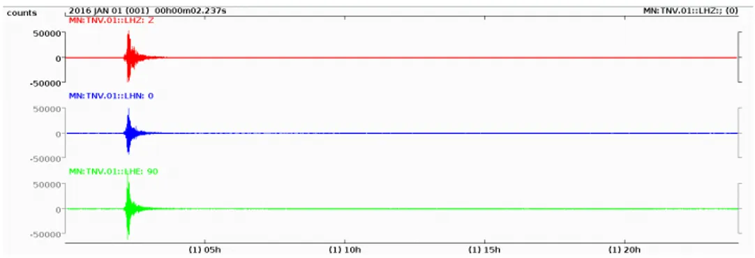
I retrieved a full copy of all the available seismic data to brought back to Italy and be made available to the scientific community. I verified the consis-tency of this dataset against the list of known seismic events happened during the previous year reported intable 1.2. As an example,figure 1.16shows the Western Indian-Antarctic Ridge earthquake happened on 1 January 2016 as recorded by the STS-1 acquisition chain.
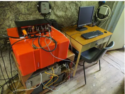
A central part of the field activities has been the replacement of the faulty and obsolete Quanterra Q4120 with the modern Quanterra Q330HR shown infigure 1.17. I removed the old instrument with its cables and sent it back to Italy. The removal of the cables has been very hard as they were completely embedded in the ice which formed over the year on the cave’s walls. I then proceeded to install the Q330HR, configuring it according to the rest of the observatory’s systems. In order to complete the installation it has been necessary to install a new GPS antenna on the outside of the cave, an operation for which logistical support has been needed. The GPS antenna RF cable has been installed in a UV resistant duct.
Figure 1.16 The 24-hour seismic of the STS-1 acquisition chain showing the 1
UTC time Lat Lon Depth Mag Location
2015-02-13 18:59:12 52.6487 -31.9016 16.68 7.1 Northern Mid-Atlantic Ridge 2015-02-27 13:45:05 -7.2968 122.5348 552.1 7 130 km N of Nebe, Indonesia 2015-03-29 23:48:31 -4.7294 152.5623 41 7.5 53 km SE of Kokopo (PNG) 2015-04-25 06:11:25 28.2305 84.7314 8.22 7.8 36 km E of Khudi, Nepal 2015-05-05 01:44:06 -5.4624 151.8751 55 7.5 130 km SSW of Kokopo (PNG) 2015-05-07 07:10:19 -7.2175 154.5567 10 7.1 143 km SW of Panguna (PNG) 2015-05-12 07:05:19 27.8087 86.0655 15 7.3 19 km SE of Kodari, Nepal 2015-05-30 11:23:02 27.8386 140.4931 664 7.8 189 km WNW of Chichi-shima (JP) 2015-06-17 12:51:32 -35.3639 -17.1605 10 7 Southern Mid-Atlantic Ridge 2015-07-18 02:27:33 -10.4012 165.1409 11 7 83 km WNW of Lata (SB) 2015-07-27 21:41:21 -2.6286 138.5277 48 7 228 km W of Abepura, Indonesia 2016-01-01 02:00:39 -50.5751 139.4469 10 6.3 Western Indian-Antarctic Ridge
2016-01-03 23:05:22 24.8339 93.6556 55 6.7 29 km W of Imphal, India
Table 1.2 Reference seismic events used to quickly assess the reliability of the
seismic data retrieved during the 31st antarctic expedition. The coordinates are in degrees, the depths in kilometers.
Figure 1.17 The overhauled TNV acquisition system. The big orange box is an old
The data acquisition server installed in the cave has been replaced with an ALPHA2000 PrioComP: a rugged, fanless system developed to be installed in demanding environments. The main storage of this system constituted on a 4 GiB industrial Compact Flash for the operating system and on a 32 GiB one for the data. I installed the Debian GNU/Linux 8.2 operating system and the SeisComP acquisition software, configured to acquire data from both the acquisition chains. The server is powered by the 12 V battery pack that powers the rest of the instrumentation, it is therefore protected from temporary issues with the diesel generators. On the server I wrote and installed a script to send the data to Italy using the Hermes system (detailed later) on a daily basis. This script takes into account the possibility of power or connectivity outages.
The backup servers installed within Mario Zucchelli station acquire and store data from both the acquisition chains. These server also offer a web interface that allows to locally view the acquired seismic data almost in real time. The acquisition is therefore done in parallel by three servers: one directly installed in the seismic cave and two installed at the station. In this configuration the possibility of experiencing a significant data loss is extremely remove.
While installing the new instrumentation in the seismic cave it became apparent that the flooded lead-acid backup batteries were not holding a charge anymore. I disposed of and replaced them; backup power is now provided by three 85 Ah Sonnenschein gel lead-acid batteries connected in parallel. The UPS installed in the cave and powering the Ethernet switch and the HDSL modem has been replaced with a better 1500 VA APC SmartUPS connected to an external battery pack.
After installing the new Quanterra Q330HR digitizer and the new acqui-sition server I verified the centering of the seismometers and the status of the vacuum chambers the STS-1s are installed in to prevent noise from con-vection in the surrounding air. The mass offsets were found in the expected value range, considered that the previous centering had been done on year before. From this point of view, the sensors were found in perfect working order. There were no problems in centering the masses, the results of the operation is summarized intable 1.3. The pressure in the vacuum chambers
the STS-1 sensors are installed in was found very good for the North and East components (86 mbar and 158 mbar respectively), while not as good for the vertical component, at 837 mbar. After evacuating the vacuum cham-pers (figure 1.13) the pressure for all the three components was less than 100 mbar.
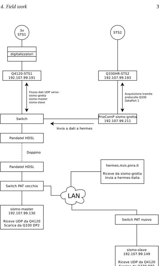
At the end of the expedition, the seismic observatory acquires, saves and automatically sends to Italy the seismic data acquired by the two acquisition chains in a stable and reliable way. The diagrams of the new data acquisition setup (figure 1.18) and power system (figure 1.18) were submitted as part of the campaign’s annual report (PNRA2016).
Activities at Concordia
The campaign at Concordia has been relatively short (less than 10 days), as the planned activities were mostly ordinary:
• Prepare a complete report of the working status of the instrumentation of the CCD observatory and of the INGV acquisition servers;
• Retrieve the seismic data of the previous year;
• Check the quality of the recorded data of the past year, verifying the absence of gaps or other kind of disturbances;
• Write and install a script that automatically sends the daily data to Italy using the Hermes system;
• Compile a general inventory.
Sensor Offset 1st centering 2nd centering STS-1 Z 3.6 V 0.1 V < 0.1 V STS-1 N 0.1 V STS-1 E 0.1 V STS-2 Z 1.9 V 0.5 V 0.6 V STS-2 N 2.5 V 0.2 V 0.4 V STS-2 E 1.8 V 0.7 V 0.8 V
Table 1.3 Centering parameters of the instruments of the Terra Nova Bay seismic
3x STS1 STS2 digitalizzatori Q4120-STS1 192.107.99.191 Q330HR-STS2 192.107.99.193 PrioComP sismo-grotta 192.107.99.211 Switch
Flusso dati UDP verso: sismo-grotta sismo-master sismo-slave Acquisizione tramite protocollo Q330 DataPort 1 Pandatel HDSL Pandatel HDSL Doppino
Switch PAT vecchio
LAN
sismo-master 192.107.99.130 Riceve UDP da Q4120 Scarica da Q330 DP2 sismo-slave 192.107.99.149 Riceve UDP da Q4120 Scarica da Q330 DP3 Switch PAT nuovo hermes.mzs.pnra.it Riceve da sismo-grottaInvia a hermes-italia Invia a dati a hermes
Figure 1.18 Diagram of the two data acquisition chains of the TNV seismic
Linea PAT 230V Alim. Elind 13.8V Batterie 3x Sonnenschein 12V 85Ah in parallelo PrioComP sismo-grotta 192.107.99.211 Quanterra Q4120 192.107.99.191 Quanterra Q330HR 192.107.99.193 STS2 UPS APC Smart-UPS 1500 Modem Pandatel Alimentatore 24V in scatola a muro Alimentatore 24V in scatola a muro Batterie 2x Sonnenschein 12V 85Ah in serie 3x STS1 Switch Ethernet
Figure 1.19 Diagram of the redundant power system of the TNV seismic
observa-tory after the 31st PNRA expedition as attached to the expedition report.
Once at Concordia, it became immediately apparent that the replacement of a Quanterra Q4120 digitizer with a newer Quanterra Q330S happened in the last days of the previous year’s summer campaign interfered with one of the the two branches of the acquisition system.
After studying the new setup I set up a new acquisition server, config-ured it to acquire data from the new digitizer and installed it in the shelter, connecting it to the local battery backed-up power line. This acquisition server is analogous to the one installed at Terra Nova Bay. It relies on a 30 GiB compact flash for both the operating system (Debian GNU/Linux 7) and the data storage. This computer also sends the daily data to Italy using the Hermes system and sends a daily email report about the data transfer. The Hermes script cleanly handles failed transfers due to power or network problems.
After the replacement of the Q4120 with a Q330S the configuration of the two INGV backup servers already present at Concordia did not correspond to the upgraded instrumentation installed at the observatory. Moreover,
these servers suffered from some hardware issues during the 2015 austral winter. I managed to fix one server using spare parts taken from the other. This server was reconfigured to acquire and store the data and host a website that graphically shows the seismic signal to the local Intranet almost in real time. This server is now installed in Concordia’s quiet building.
The data acquired during 2015 have been saved in double copy, quality checked against a list of known seismic events and brFought to Italy.
During all these operations I trained the overwintering electronics tech-nician for science of the 12th winter campaign on the activities to carry on during the winter in order to keep all the systems up and running.
The status before leaving Concordia is the following: the data is correctly acquired, saved locally and regularly sent to Italy in an automatic way. Up to this point, there was no need for any manual intervention, and all the systems appear stable and reliable.
The Hermes data transfer system
Hermes (High Efficiency Relay of Mission Experiments data Sharing) is a system to transfer scientific data from the Antarctic stations to Italy which I developed during the 10th PNRA winter campaign in Concordia and the 31 PNRA summer campaign. This section summarizes the way it operates, more information is available in the annual expeditions reports (PNRA
2015a,2016).
Hermes has been developed from the need to transfer scientific data from Concordia to Europe and to make them available to the interested parties. An ad-hoc system is necessary as the bandwidth available to the Antarctic stations is heavily limited: in the case of Concordia a VSAT4link provides a 512 Kibit/s connection to the Internet. The satellite link is not stable and suffers from a very high latency (from hundreds of milliseconds to several seconds, when the link is congested). An effort towards the implementation of a scientific data transfer system had already been done by the electronic technician for science of the 9th winter campaign in Concordia, A. Litterio, but his implementation relied on very different tools from the ones I’ve used.
4. A very small aperture terminal (VSAT) is a two-way satellite ground station with a dish antenna that is smaller than 3.8 m.
However, I kept the name he chose for the system: Hermes.
The basic idea behind the system is to centralize the data transfers, in-stalling a pair of servers: one in Italy and one in the Antarctic base. Hermes transfers the data from the server in Antarctica to the one in Italy in an automatic an reliable way, minimizing the bandwidth usage. Because of the bandwidth constrains the system has been developed to:
1. Resume the interrupted data transfers, in order not to waste bandwidth because of the (relatively frequent.) connectivity outages;
2. Avoid to transfer the same data more than once, regardless of what the users of the system do;
3. Compress the data to transfer as much as possible, without relying on the the users doing so.
These needs and the general logistical limitations brought to some technical choices:
• Use standard tools available in any GNU/Linux distribution in order make it possible to use the system regardless of the particular distribu-tion in use;
• Avoid polling for new data, and start the transfer as soon as some new data is available;
• Use a public key authentication system to authorize the data trasnfers. In practice, Hermes is a set of interacting scripts leveragingcron,inotify,
rsync,sshandsftp.Figure 1.20schematically shows how the system oper-ates, the full documentation on the system is part of the reports I produced after the expeditions and is available inappendix A(in Italian). The docu-mentation cover also the topics of the accounting and tipe-dependent traffic shaping.
Data consolidation effort
The Terra Nova Bay seismic observatory (TNV), being operative since the 1988–1989 antarctic summer, is one of the longest-running observatories of
Data Acquisition Local HERMES server
Internet
Italian HERMES server Ground station
Sensor
Figure 1.20 Schematic diagram of the Hermes system. When new data is
trans-ferred to the local Hermes server the data transfer to the Italian Hermes server is initiated. The peculiarity of the system is the resilience to outages, the tolerance to very high latencies, the transparent compression and the avoidance of duplicate data transfers.
the continent. The site and instrumentation are excellent and it has a long record of yearly maintenance operation, with relatively few gaps in the data. After a careful reprocessing, cleanup and consolidation work I have done in collaboration with Dr. P. Danecek of INGV Rome, the data from TNV will soon be available in the International Federation of Digital Seismograph Networks (FDSN). This progress was brought to the 36th General Assembly of the European Seismological Commission:
P. Danecek, A. Delladio, D. Zigone, A. Cavaliere, P. Legovini, and D. Sor-rentino (2018). Seismological Observatories in Antarctica: An Update on the Italian Program and the Evolution of the Observatories. Poster. Pre-sented 36th General Assembly of the European Seismological Commission (ESC2018), Malta (MT).
Noise interferometry
2.1
Seismic noise
Definition
In the absence of earthquakes, seismometers record a wide range of signals generated from both natural and anthropogenic sources as well as from the instruments themselves. As these signals interfere with our ability to record earthquakes, which historically generated the only signal of interest to seismologists, they have been grouped together and given the term noise. This situation is schematically shown infigure 2.1. Noise can be divided into three broad categories:
(i) self-noise of seismic instruments; (ii) non-seismic noise sources;
(iii) non-earthquake sources of seismic energy.
The self-noise of the seismometer and digitizer(i)arises from their elec-tronics and from thermally induced motions on the seismometer’s mass. Self-noise often increases drastically at lower frequencies. Non-seismic noise sources(ii)arise because seismic instruments are sensitive to environmental conditions such as thermal variations, magnetic fields, and changes in the atmospheric pressure. Finally, non-earthquake sources of seismic energy
(iii)arise from a multitude of naturally occurring surface processes as well as human activities. In this latest meaning the word noise is partially a historical
Figure 2.1 One day of seismic record showing the source-dependent, directive waves from an earthquake (also called ballistic waves) and seismic noise before and after the event.
misnomer: while seismologists were not very interested in this kind of signal and did normally try to get rid of it, it still is a physical signal to all effects. A more precise name could be “microseismic signal”, however in what follows we will refer to this signal as “ambient seismic noise”, “ambient wavefield” or simply as “seismic noise.”
In recent years it has emerged that ambient seismic noise is far from useless: it has been demonstrated theoretically and in practice that by ap-plying the signal processing techniques described in this chapter to pairs of ambient noise records made at the Earth’s surface, useful information about the seismic properties of the subsurface can be obtained: this process is known as seismic noise interferometry (Shapiro2005; Shapiro and Campillo
2004; Weaver2005).
Sources of ambient seismic noise
Ambient seismic noise consists mostly of surface waves and is due to a number of causes. Higher frequency seismic noise (above 1 Hz) is mainly anthropogenic, originating from activities like road traffic and industrial work. Vibrations at around 1 Hz originate from the interaction between the solid earth and the atmosphere, and are mainly due to wind and other
atmospheric phenomena. Lower frequency noise (below 1 Hz) come from the interaction between the solid earth and the hydrosphere, and in particular from the ocean waves (Bonnefoy-Claudet, Cotton, and Bard2006).
The longer-period end of the noise spectrum shows different features. At about 𝑇 = 14 s we have the primary microseismic peak, while at about 𝑇 = 7 s we have the secondary microseismic peak. The energetic peak located beyond 𝑇 = 30 s is referred as seismic hum. A spectral plot displaying this subdivision is shown in figure 2.2. The distinction between the primary peak and secondary peak is due to the different noise generation mechanism (Stehly, Campillo, and Shapiro2006).
2.2
From noise to the Green’s function
Green’s functions
In mathematics, a Green’s function 𝐺(𝑡) is the impulse response of an inho-mogeneous linear differential equation defined on a domain with specified initial conditions or boundary conditions. From the physical point of view, the Green’s function 𝐺(𝑥, 𝑠, 𝑡) gives the displacement of a point 𝑥 due to an impulsive force 𝛿(𝑡) located in 𝑠 (Bayin2018).
Over the time scales of seismic wave propagation we can consider Earth as a linear and invariant system: it is linearly elastic and its physical properties (density and elastic moduli) are constant. For this reason the response of the system to a linear superposition of pulses 𝑎𝛿(𝑡) + 𝑏𝛿(𝑡 − 𝑡′) is 𝑎𝐺(𝑡) + 𝑏𝐺(𝑡 −
𝑡′). An arbitrary force 𝑓 (𝑡) can always be expressed as a superposition of
impulses:
𝑓 (𝑡) = ∫ 𝑓 (𝑡′)𝛿(𝑡 − 𝑡′) d𝑡′ = [𝑓 ∗ 𝛿](𝑡)
where the asterisk is the convolution operator. It is then clear that the Green function contains the information on the response of the system to an arbi-trary force 𝑓 (𝑡). This response is given by:
∫ 𝑓 (𝑡′)𝐺(𝑡 − 𝑡′) d𝑡′= [𝑓 ∗ 𝐺](𝑡).
When the system under analysis is an elastic medium, the Green’s function contains all the information needed to describe how waves propagate in the
Figure 2.2 Probability density function of power spectral density (PSD) for the vertical-component of South Pole station QSPA (146 m borehole) for December 2007 to December 2012 plotted on a logarithmic scale (modified from Anthony et al.
system (Bayin2018).
In seismology, the Green’s function between a pair of locations describes the seismic energy which would result at one if there was an impulsive seismic source at the other. In other words, the Green’s function describes the effect of the medium between the two locations on an impulsive source, and contains traveltime and waveform information about all the seismic phases that pass between the two locations (Stein and Wysession2003). The Green’s function can be thought as the seismogram which would be recorded at some location in response to a source at another.
Cross-correlation
In signal processing, the cross-correlation is a measure of similarity of two time series as a function of the displacement of one relative to the other. Its most common application is searching for a known feature in a much longer signal. For continuous, real-valued functions 𝑓 (𝑡) and 𝑔(𝑡), the cross-correlation is defined as:
𝐶𝑓 𝑔(𝜏) = [𝑓 ⋆ 𝑔](𝜏) = ∫+∞
−∞ 𝑓 (𝑡)𝑔(𝑡 + 𝜏) d𝑡, (2.1)
where 𝜏 is the displacement (or lag time) between the functions. In the case of two real-valued discrete signals the cross-correlation is defined as:
𝐶𝑓 𝑔(𝜏) = (𝑓 ⋆ 𝑔)(𝑛) =
+∞
∑
𝑡=−∞
𝑓 (𝑡) 𝑔(𝑡 + 𝜏) (2.2)
where 𝑓 , 𝑔 are two time-series (signals) and 𝜏 is the lag time.
When 𝑓 and 𝑔 are similar signals the cross-correlation function is peaked at lag times for which the signals are best aligned. A cross-correlation of a signal with itself (autocorrelation) therefore has its maximum for a time lag of zero. Signals without similarities will produce a cross-correlation function that has a small amplitude for any lag time because the integrated product averages to zero.
In seismology it is useful to think the cross-correlation as a way to high-light the traveltime of seismic waves. A wavefield which has travelled be-tween two stations will cause a similar signal to be recorded at each, shifted in time: the cross-correlation function of the records will therefore contain
a peak at a time lag which corresponds to the traveltime of the wavefield between the two stations.
Equations (2.1)and(2.2)are general mathematical definitions, but in practical applications the signals are defined over a finite time interval 𝑇 and it is often useful to work with normalized correlation values. We can then define the geometrically normalized cross-correlation (CCGN) of two seismic signals as 𝐶ccgn(𝜏) = ∑ 𝑡0+𝑇 𝑡=𝑡0 𝑓 (𝑡)𝑔(𝑡 + 𝜏) √∑𝑡0+𝑇 𝑡=𝑡0 𝑓 2(𝑡) ∑𝑡0+𝑇 𝑡=𝑡0 𝑔 2(𝑡 + 𝜏) (2.3)
where the symbols have the same meaning as inequation (2.2). The denom-inator ofequation (2.3)is the geometrical mean of the energy within the time window 𝑇 and normalizes the cross-correlation: we have |𝐶ccgn| ≤ 1, with 𝐶ccgn= 1 in the case of perfect correlation and 𝐶ccgn= −1 in the case of perfect anticorrelation.
Noise cross-correlation
There is an important theoretical result that binds the cross-correlations of seismic noise and the Green’s functions. If the noise field is diffuse (isotropi-cally distributed) and equipartitioned (all the oscillation modes are equally excited), then the cross-correlation of such a noise field recorded at the loca-tions 𝐴 and 𝐵 is related to the Green’s funcloca-tions 𝐺𝐴𝐵and 𝐺𝐵𝐴between the two points as follows
d𝐶𝐴𝐵
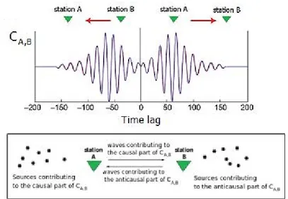
d𝑡 = −𝐺𝐴𝐵(𝑡) + 𝐺𝐵𝐴(−𝑡). (2.4) and schematically shown infigure 2.4. In an ideal situation 𝐺𝐴𝐵and 𝐺𝐵𝐴 are symmetrical because of the symmetry of the system, although in prac-tice, when the noise distribution is not perfectly homogeneous, they may slightly differ. The negative and positive time lags correspond to noise sig-nals traveling from 𝐵 to 𝐴 and 𝐴 to 𝐵, respectively. The usefulness of this result has been first demonstrated by Lobkis and Weaver (2001) in the field of high frequency acoustic waves, already envisioning the applications in seismology, while Wapenaar (2004) first showed the retrieval of the Green’s
function of an arbitrary inhomogeneous medium by cross correlation. Cross-correlation is performed for positive and negative time lags, so the cross-correlation functions have both positive (causal) and negative (acausal) components (figure 2.5). Seismic noise arrives from all directions, and the noise records which are cross-correlated therefore contain energy which has travelled in both directions along an interstation path. The Green’s functions calculated from equation (2.4)will therefore contain energy in both the causal and acausal parts, symmetric about zero time lag: the causal part representing energy arriving at station 𝐵 in response to an impulsive source at station 𝐴, and the acausal part energy arriving at station 𝐴 in response to a source at station 𝐵. Because the Green’s functions are the same in both directions along a path, the two sides of the noise cross-correlation function can be treated as representing the same information. In reality a noise cross-correlation function will be perfectly symmetrical only if noise arrives from both sides of the interstation path with equal strength, which is rarely the case in practice.
In order to retrieve the complete Green’s functions, which contain the whole suite of seismic waves caused by an impulsive seismic source, the required random sources must be equally distributed in the subsurface (Wapenaar2004). As we said, this ideal condition is not verified in prac-tice, but it has been shown (Shapiro2005) that even in the non-ideal case the Green’s functions can be at least partially reconstructed using seismic noise interferometry with the same accuracy of “traditional” earthquake observations.
Correlogram stacks
The correlation is normally done by dividing the data in time windows; the correlation is then computed on individual window pairs, and the correlo-grams are then stacked (summed), so their coherent part is amplified, while the incoherent part averages to zero. This classic workflow is shown schemat-ically infigure 2.6, while a stack of cross-correlation obtained from a pair of stations in Antarctica is shown infigure 2.7. It is important to underline that in this study we are interested in the arrival times of the different phases of the seismograms, disregarding their amplitudes. For this reason there are no
Figure 2.3 Representation of a diffuse noise field (modified from Weaver2005). The two detectors normally record a random signal, waves that pass through both the detectors (like the red arrow) constitute a component of the two signals that is coherent and can be detected by cross-correlating them.
Figure 2.4 Schematic view of the principle of the seismic interferometry method.In
the case of a diffuse noise field (left), the cross correlation of the signal recorded at A and B allows to derive the Green’s function between the two locations (right).
Figure 2.5 Causal and acausal parts of an noise cross-correlation function. Top: idealized noise cross-correlation function for a wavefield propagating from station 𝐴 to station 𝐵. The arrows indicate the energy path which is represented by the positive and negative parts of the cross-correlation function. Bottom: representation of the noise sources which contribute to the causal and acausal components of the cross-correlation function.
problems in altering the amplitudes by stacking signals (even non-linearly, as we shall see) or normalizing. The only important thing is to keep the amplitude within the stability limits of the numerical tools.
Applications in seismic tomography
Seismic tomography has been developed on data coming from seismic events (earthquakes). The usage of earthquake data allows for an excellent tomo-graphic analysis, as seismic waves from earthquakes are very energetic and hence it is relatively easy to detect them and extract the high amount of information they contain. At the same time the exact location of earthquake is often not perfectly determined: localizing the hypocenter of the event is not trivial, the localization depends in part on the chosen 3D model, and faults are not point-sources but are extended. Moreover, there is a number of different seismogenic mechanisms. All these effects contribute to diminish the imaging power of the tomographies computed using earthquake data.
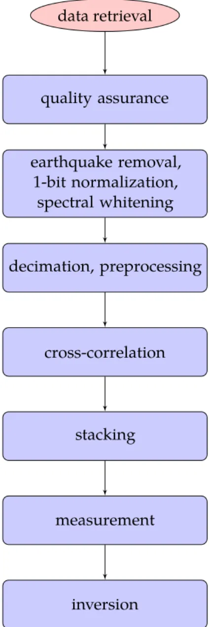
data retrieval quality assurance earthquake removal, 1-bit normalization, spectral whitening decimation, preprocessing cross-correlation stacking measurement inversion
Figure 2.6 The stages of a simple seismic interferometry workflow based on the
Figure 2.7 A stack of cross-correlations for a pair of stations in Antarctica. The quantity in abscissa in a stack (sum) of cross-correlation coefficients. Note that the function is not perfectly symmetrical, as it was in the ideal case offigure 2.5. This is because in reality the noise field is not perfectly homogeneous.
station in any point of the planet can record it, so the data availability is virtually infinite. This is especially important in areas characterized by a low seismic activity, like the Antarctic continent.
The noise cross-correlation technique had a great impact in the scientific production of the last ten years, with several important published results, among the others: Lu et al. (2018), Nishida, Montagner, and Kawakatsu (2009), Poli, H. A. Pedersen, and and (2011), Ritzwoller, Lin, and Shen (2011), Shapiro (2005), Yao, Beghein, and Hilst (2008), and Yao, Hilst, and Hoop (2006). More specifically about Antarctica a relevant work is An et al. (2015), where a continental scale tomography is computed using classical noise cross-correlation data complemented with earthquake data.
2.3
The phase cross-correlation
Definition
The phase correlation (PCC) is a coherence measure akin to the cross-correlation as defined insection 2.2, but whileequation (2.2)is based on the signals’ amplitude, the PCC is based on the similarity of their instantaneous
phases. The PCC has been developed to evaluate the goodness of waveform fit between two time series as function of lag time by Schimmel (1999) and later used for interferometric studies, for example by Schimmel, Stutzmann, and Gallart (2011).
The basic idea of the phase cross-correlation is to use the phase of a complex function as the correlation variable instead of its amplitude. The signals we are interested in are real time-series, so to introduce the concept of phase we need to bring them in the complex domain. This is done by constructing their analytic representation. Given a real-valued signal 𝑠(𝑡), its analytic representation 𝑆(𝑡) is a complex signal which has 𝑠(𝑡) as its real part and the Hilbert transform of 𝑠(𝑡) as its imaginary part:
𝑆(𝑡) = 𝑠(𝑡) + iℋ[𝑠(𝑡)].
𝑆(𝑡) is an analytic signal, that is: a complex-valued function that has no negative frequency components. As any complex function 𝑆(𝑡) can always be written in exponential form
𝑆(𝑡) = 𝐴(𝑡)ei𝜙(𝑡) (2.5) where 𝐴(𝑡) is called the envelope of 𝑆(𝑡) and 𝜙(𝑡) its instantaneous phase, which will be our correlation variable (Schimmel1999).
Given two signals of length 𝑇 with instantaneous phases 𝜙(𝑡) and 𝜓(𝑡), their phase cross-correlation is defined as (Schimmel1999):
𝐶pcc(𝜏) = 1 2𝑇
𝑡0+𝑇
∑
𝑡=𝑡0
[∣ei𝜙(𝑡)+ 𝑒i𝜓(𝑡+𝜏)∣ − ∣ei𝜙(𝑡)− ei𝜓(𝑡+𝜏)∣]
which is a coherence measure with the same normalization properties of
equation (2.3).
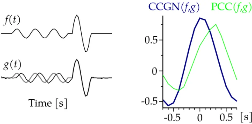
Comparison with the classic correlation
One important difference between the classic cross-correlation and the phase cross-correlation consists in the fact that the classic cross-correlation favors the similarity between high amplitude features in the signals, while the