Flow around a circular cylinder
at
Re
D
= 3900. Coarse grid
3.1
Description of the test case
VMS-LES approach is adopted here to simulate the flow past a circular
cylinder at Mach number M∞ = 0.1 and at a subcritical Reynolds number
ReD of 3900 (ReD =
u∞D
ν ) based on cylinder diameter D and free-stream
velocity u∞.
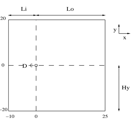
With reference to Figure 3.1, the computational domain dimensions are −10 ≤ x/D ≤ 25, −20 ≤ y/D ≤ 20 and −π/2 ≤ z/D ≤ π/2 where x, y and z denote the streamwise, transverse and spanwise directions respectively, and:
Li/D = 10, L0/D = 25, Hy/D = 20 and Hz/D = π
The cylinder of unit diameter is centered on (x,y) = (0,0).
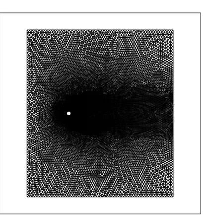
The surface of the cylinder has been divided into 160 parts in the tangen-tial direction and 30 parts in the z direction. An unstructured grid has been created with 290498 nodes and 1580392 elements. A vertical cut-plane of this rather coarse mesh and a zoom around the cylinder are shown in Figure 3.2. The average distance of the nearest point to the cylinder boundary is
0.017D which corresponds to y+ ≈ 3.31.
20
D
−20
0
−10
0
Li
25
Lo
Hy
x
y
3.2
Results of the simulations
The Steger-Warming conditions [14] are imposed at the inflow and outflow
as well as on the upper and lower surface (y = ± Hy). In the spanwise
direction periodic boundary conditions is applied. On the cylinder surface no-slip boundary conditions are set.
To investigate the influence of different subgrid scale models on the VMS-LES approach, three simulations are carried out on the same grid: VMS-VMS-LES with classical Smagorinsky SGS model (Smago.), VMS-LES with Vreman SGS model (Vreman) and VMS-LES with WALE SGS model (WALE). Two other simulations are carried out in order to show the impact of precondi-toning on VMS-LES computation at the considered Mach number, using the Smagorinsky and the WALE models. The preconditioning used for both sim-ulations is the Roe-Turkel solver described in [15]. The high-order viscosity scheme presented in section 2.3 is used with a numerical viscosity parameter γ set to 0.3.
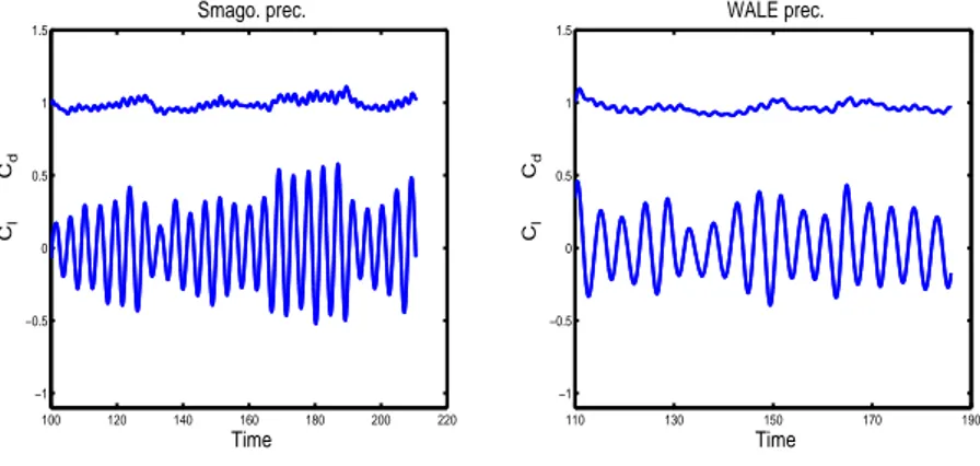
The flow equations are advanced in time with the second-order time ac-curate implicit scheme described in section 2.6. The CFL number has been chosen such that about 1000 time steps are used for each vortex shedding cycle. The averaged data are obtained over about 22 shedding cycles or 100 nondimensional time units after the initial transient period. The drag and lift history of the simulations with and without preconditioning are shown in Figure 3.3 and Figure 3.4 respectively.
Time-averaged values and bulk flow parameters are summarized in Ta-ble 3.1 and compared to data from experiments of Son and Hanratty [16],
Norberg [17], Cardell [18] and Williamson [19]. Cd denotes the mean drag
coefficient, C′
d and C
′
l respectively the root mean square values of the drag
and lift, St the Strouhal number, lr the mean recirculation length from the
surface of the cylinder, i.e. the distance at point along the centerline where the time-averaged streamwise velocity is zero, θsep the separation angle and
The Strouhal number St = f Du∞ is based on to the velocity u∞ and the
diameter D. The local velocity of the flow is nondimensionalized with u∞
velocity,while the recirculation lenght lr is made non-dimensional with the
diameter D.
Data from St Cd Cd′ Cl′ lr θsep umin
Smago. 0.219 1.18 0.0842 0.497 0.89 95 -0.28 Vreman 0.212 1.17 0.0750 0.483 0.94 93 -0.31 WALE 0.215 1.23 0.0639 0.592 0.92 93 -0.26 Smago. prec. 0.221 0.99 0.0359 0.259 1.11 87 -0.29 WALE prec. 0.220 0.96 0.0274 0.196 1.17 87 -0.27 Numerical data [22] 0.210 1.04 1.35 -0.37 [24] 1.07 1.197 87.7 [25] 0.212 0.99 1.36 -0.33 Experiments [18], [17], [16] 0.215±0.05 0.99±0.05 1.33±0.02 85±2 -0.24±0.1 [19], [26] 0.21±0.05 1.18±0.05
Table 3.1. Bulk flow parameters
As shown in Table 3.1, for the simulations without preconditioning, the Strouhal number and the minimum centerline velocity are in good agreement with the experimental values and we notice that the other parameters are less well predicted. The recirculation length is underestimated, the mean drag coefficient and the separation angle are larger than the experimental data. The results show that preconditioning improves the quality of the simulation, since all parameters are well predicted and moreover when preconditioning is used, the influence of the SGS model on the results is reduced.
Figure 3.5 and Figure 3.6 show the time-averaged streamwise velocity on the centerline direction of the no-preconditioned and preconditioned simu-lations respectively. Figure 3.5 shows a slight influence of the subgrid scale model; indeed, the results obtained in the WALE simulation are slightly better. It appears that the recirculation length of the no-preconditioned simulations are smaller than expected. The preconditioning improves the results. Figure 3.6 shows that the simulations with preconditioning are in
accordance with the experiments of Lourenco and Shih (data from Beaudan and Moin [20]) and Ong and Wallace [21].
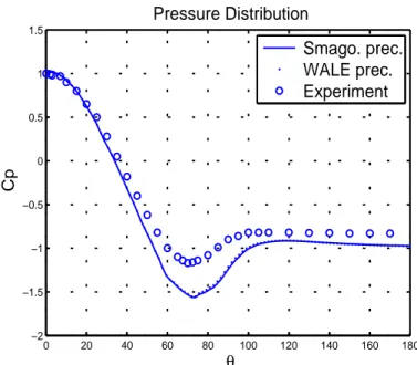
Figure 3.7 and Figure 3.8 show the pressure distribution on the cylinder surface averaged in time and on the homogeneous z direction obtained in the non-preconditioned and preconditioned simulations respectively. In the no-preconditioned case, the Smagorinsky, WALE and Vreman results are very close each other on the whole cylinder. The better results are again obtained with preconditioning but it appears a deviation respect to the experimental data from Norberg [17]. Comparisons between Figure 3.7 and Figure 3.8, preconditioning is crucial at the stagnation point significantly reducing the gap between the obtained cpm value and the theoretical one. In Figure 3.8, the discrepancies between 60 and 80◦
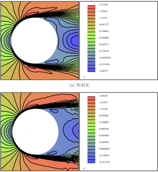
may be explained by the rather coarse grid used. The timed-averaged streamwise velocity of the WALE simulation and WALE preconditioning simulation are plotted in Figure 3.13. It appears that the angle of separation in the preconditioned simulation is smaller and closer to the experimental value from Son and Hanratty [16], Norberg [17] and Cardell [18] in Table 3.1.
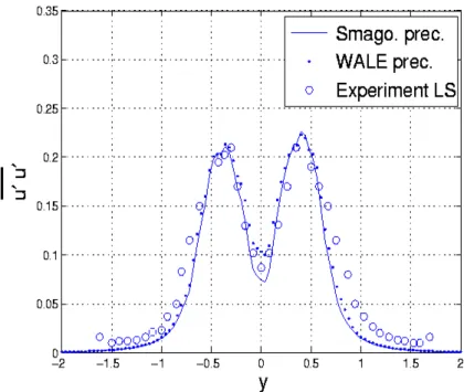
Figure 3.9 and Figure 3.10 display the total resolved Reynolds stress u′u′ at x = 1.54 using different subgrid scale models with preconditioning and without preconditioning respectively. In Figure 3.9, the first peak is overpredicted by Smagorinsky and Vreman simulations whereas the WALE simulation correlates well with the experimental data of Lourenco and Shih (data from Beaudan and Moin [20]). The preconditioned simulations yield better results, as shown in Figure 3.10.
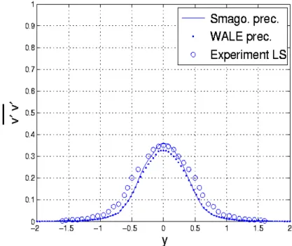
Figure 3.11 and Figure 3.12 shows the total resolved Reynolds stress v′v′ at x = 1.54 using different subgrid scale models with preconditioning and without preconditioning respectively. Without preconditioning the WALE simulation shows an excellent agreement with the experimental values of Lourenco and Shih, whereas Smagorinsky and Vreman simulations highly overpredict the Reynolds stress v′v′. Again, the preconditioned simulations are closer to the experimental values with less influence of the subgrid scale
model. 100 150 200 250 −1 −0.5 0 0.5 1 1.5 Time C l C d Smago. 60 100 140 180 220 −1 −0.5 0 0.5 1 1.5 Time C l C d WALE 40 60 80 100 120 140 160 180 −1 −0.5 0 0.5 1 1.5 Time C l C d Vreman
Figure 3.3. Lift and Drag coefficient history without preconditioning
100 120 140 160 180 200 220 −1 −0.5 0 0.5 1 1.5 Time C l C d Smago. prec. 110 130 150 170 190 −1 −0.5 0 0.5 1 1.5 Time C l C d WALE prec.
0.5 1 1.5 2 2.5 3 3.5 4 4.5 5 5.5 6 6.5 7 7.5 8 8.5 9 9.5 10 −0.4 −0.2 0 0.2 0.4 0.6 0.8 1
Time−Averaged Streamwise Velocity
x U Smago. Vreman WALE Experiment LS Experiment OW
Figure 3.5. Time-averaged streamwise velocity on the centerline obtained in the simulations without preconditioning. Experiments: Lourenco and Shih (LS) [20] and Ong and Wallace (OW) [21]
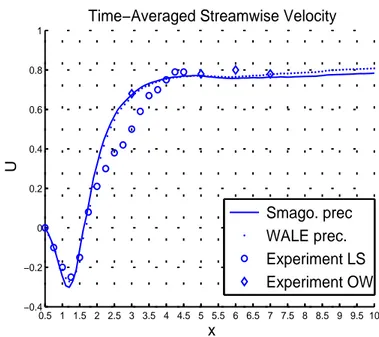
0.5 1 1.5 2 2.5 3 3.5 4 4.5 5 5.5 6 6.5 7 7.5 8 8.5 9 9.5 10 −0.4 −0.2 0 0.2 0.4 0.6 0.8 1 x U
Time−Averaged Streamwise Velocity
Smago. prec WALE prec. Experiment LS Experiment OW
Figure 3.6. Time-averaged streamwise velocity on the centerline obtained in the simulations with preconditioning. Experiments: Lourenco and Shih (LS) [20] and Ong and Wallace (OW) [21]
0 20 40 60 80 100 120 140 160 180 −2 −1.5 −1 −0.5 0 0.5 1 1.5 θ Cp Pressure Distribution Smago. Vreman WALE Experiment
Figure 3.7. Time-averaged and z-averaged pressure distribution on the surface of the cylinder obtained in the simulations without preconditioning. Experiment: Norberg [17] 0 20 40 60 80 100 120 140 160 180 −2 −1.5 −1 −0.5 0 0.5 1 1.5 θ Cp Pressure Distribution Smago. prec. WALE prec. Experiment
Figure 3.8. Time-averaged and z-averaged pressure distribution on the surface of the cylinder obtained in the simulations with preconditioning. Experiment: Norberg [17]
Figure 3.9. Total resolved streamwise Reynolds stress u′u′ at x = 1.54 without preconditioning. Experiments: Lourenco and Shih (LS) [20]
Figure 3.10. Total resolved streamwise Reynolds stress u′u′ at x = 1.54 with preconditioning. Experiments: Lourenco and Shih (LS) [20]
Figure 3.11. Total resolved transverse Reynolds stress v′v′ at x = 1.54 without preconditioning. Experiments: Lourenco and Shih (LS) [20]
Figure 3.12. Total resolved transverse Reynolds stress v′v′ at x = 1.54 with preconditioning. Experiments: Lourenco and Shih (LS) [20]
u -0.40377 -0.211634 -0.0194992 0.172636 0.364771 0.556906 0.749041 0.941177 1.13331 1.32545 1.51758 (a) WALE u -0.315718 -0.134817 0.0460833 0.226984 0.407884 0.588784 0.769685 0.950585 1.13149 1.31239 1.49329 (b) WALE prec.