A
A
l
l
m
m
a
a
M
M
a
a
t
t
e
e
r
r
S
S
t
t
u
u
d
d
i
i
o
o
r
r
u
u
m
m
–
–
U
U
n
n
i
i
v
v
e
e
r
r
s
s
i
i
t
t
à
à
d
d
i
i
B
B
o
o
l
l
o
o
g
g
n
n
a
a
Dottorato di Ricerca in Geofisica
XXIV ciclo
Integrating new and traditional approaches
for the estimate of slip-rates of active faults:
examples from the Mw 6.3, 2009 L’Aquila
earthquake area, Central Italy
Settore Concorsuale di afferenza: 04/A4/Geo10 – GEOFISICA DELLA TERRA SOLIDA
Presentata da: Riccardo Civico
Coordinatore Dottorato
Relatore
Prof. Michele Dragoni
Dott. Paolo Marco De Martini
Abstract
This thesis developed a multidisciplinary and multi-scale investigation strategy based on the integration of traditional and innovative approaches aimed at improving the normal faults seimogenic identification and characterization, focusing mainly on slip-rate estimate as a measure of the fault activity.
The L’Aquila Mw 6.3 April 6, 2009 earthquake causative fault was used as a test site for the application, testing, and refinement of traditional and/or innovative approaches, with the aim to 1) evaluate their strength or limitations 2) develop a reference approach useful for extending the investigation to other active faults in the area and 3) translate the results of the the methodological approaches as new inputs to local seismic hazard.
The April 6, 2009 L’Aquila earthquake occurred on a so far poorly known tectonic structure, considered having a limited seismic potential, the Paganica - San Demetrio fault system (PSDFS), and thus has highlighted the need for a detailed knowledge in terms of location, geometry, and characterization of the active faults that are the potential sources for future earthquakes.
To fill the gap of knowledge enhanced by the occurrence of the 2009 L’Aquila earthquake, we developed a multidisciplinary and scale-based strategy consisting of paleoseismological investigations, detailed geomorphological and geological field studies, as well as shallow geophysical imaging, and an innovative methodology that uses, as an alternative paleoseismological tool, core sampling and laboratory analyses but also in situ measurements of physical properties.
The integration of geomorphology, geology as well as shallow geophysics, was essential to produce a new detailed geomorphological and geological map of the PSDFS and to define its tectonic style, arrangement, kinematics, extent, geometry and internal complexities.
Our investigations highlighted that the PSDFS is a 19 km-long tectonic structure characterized by a complex structural setting at the surface and that is arranged in two main sectors: the Paganica sector to the NW and the San Demetrio sector to SE. The Paganica sector is characterized by a narrow deformation zone, with a relatively small (but deep) Quaternary basin affected by few fault splays. The San Demetrio sector is characterized by a strain distribution at the surface that is accommodated by several tectonic structures, with the system opening into a set of parallel, km-spaced fault traces that exhume and dissect the Quaternary basin.
The integration of all the fault displacement data and age constraints (radiocarbon dating, optically stimulated luminescence (OSL) and tephrochronology) resulting from paleoseismological, geomorphological, geophysical and geological investigations played a primary role in the estimate of the slip-rate of the PSDFS. Slip-rates were estimated for different time intervals in the Quaternary, from Early
Pleistocene (1.8 Ma) to Late Holocene (last 5 ka), yielding values ranging between 0.09 and 0.58 and providing an average Quaternary slip-rate representative for the PSDFS of 0.27 - 0.48 mm/yr.
We contributed also to the understanding of the PSDFS seismic behavior and of the local seismic hazard by estimating the max expected magnitude for this fault on the basis of its length (ca. 20 km) and slip per event (up to 0.8 m), and identifying the two most active fault splays at present. Our multidisciplinary results converge toward the possibility of the occurrence of past surface faulting earthquakes characterized by a moment magnitude between 6.3 and 6.8, notably larger than the 2009 event, but compatible with the M range observed in historical earthquakes in the area. The slip-rate distribution over time and space and the tectonic style of the PSDFS suggested the occurrence of strain migration through time in the southern sector from the easternmost basin-bounding fault splay toward the southwestern splays. This topic has a significant implication in terms of surface faulting hazard in the area, because it can contribute defining the fault splays that have a higher potential to slip during future earthquakes along the PSDFS.
By a methodological point of view, the multidisciplinary and multiscale-based investigation strategy emphasizes the advantages of the joint application of different approaches and methodologies for active faults identification and characterization. Our work suggests that each approach alone may provide sufficient information but only the application of a multidisciplinary strategy is effective in providing a proper framework of active faults and robust results.
TABLE OF CONTENTS Abstract Table of contents Acknowledgments 1. Introduction 1
2. Active faults in geology 4
2.1. Faults: basic concepts 2.1.1. Faults and stress 2.1.2. Fault growing 2.2. Active faults
2.2.1. Definition
2.2.2. Faults and slip accumulation models 2.2.3. Faults and strain release models
2.2.4. Faults geometry and regional stress field 2.2.5. Geologic evidence of active normal faults 2.2.6. Landforms associated with active normal faults
2.3. Examples from the Basin and Range Province and from the Walker Lane, Nevada, USA
2.4. Slip-rate
3. The Mw 6.3 6 April 2009 L’Aquila earthquake 24 3.1. Seismic sequence and causative fault
3.1.1. The seismic sequence
3.1.2. The earthquake causative fault: The Paganica fault 3.2. Earthquake effects on the environment
3.2.1. Coseismic deformation
3.2.2. Coseismic surface effects and ground ruptures 3.3. Summary
3.4. Open questions raised by the 2009 earthquake
3.5. Other examples of surface faulting earthquakes and coseismic deformation 3.5.1. The 2010 (Mw 7.2) El Major – Cucapah earthquake
3.5.2. The 1915 Pleasant Valley (Ms 7.7), 1954 Fairview Peak (Ms 7.2) and Dixie Valley (Ms 6.8) earthquakes and their surface ruptures
5. Paleoseismological approach 53 5.1. Introduction 5.2. Paleoseismology – method 5.2.1. Trenches 5.2.2. Coring 5.2.3. Chronological constraints 5.2.3.1. Radiocarbon dating
5.2.3.2. Archeological evaluation of pottery shards 5.3. Paleoseismological trenching along the PSDFS
5.3.1. Aqueduct site 5.3.2. Zaccagnini site 5.3.3. Mo’Tretteca site 5.3.4. 250K site
5.4. Main results
6. Tectonic geomorphological and geological approach 73 6.1. Introduction
6.2. Tectonic geomorphology approach 6.2.1. LiDAR
6.2.2. Large-scale view of the Middle Aterno basin 6.2.3. Landforms
6.2.4. Across-strike topographic profiles
6.2.5. Main results of the tectonic geomorphology approach 6.3. Geological approach
6.3.1. Geological mapping 6.3.2. Quaternary deposits 6.3.3. Chronological constraints
6.3.3.1. Optically Stimulated Luminescence (OSL) 6.3.3.2. Tephrochronology
6.3.4. Geological cross sections
7. Geophysical approach 105
7.1. Introduction
7.2. High-resolution petrophysical correlations 7.2.1. Introduction
7.2.2. Mo’Tretteca site 7.2.3. Fossa site
7.3. Electrical resistivity tomography 7.3.1. Method
7.3.2. Results
7.3.3. San Vittorino site 7.3.4. Villa Sant’Angelo site 7.3.5. L’Annunziata site 7.3.6. San Gregorio site 7.3.7. Pie’ i colle site
7.3.8. Campo di Contra site
7.4. High-resolution seismic tomography 7.4.1. Method
8. Discussion 133 8.1. Tectonic style
8.2. PSDFS length
8.3. Partitioning of deformation along the PSDFS 8.4. Slip-rate
8.5. Slip-rates through time and space 8.6. Strain migration
8.7. Contribution to seismic hazard
9. Conclusions 151 References 155 Appendix A Appendix B Appendix C Appendix D1-2-3-4 Appendix E Appendix F Appendix G Appendix H Appendix I
Acknowledgements
First and foremost I offer my sincerest gratitude to my supervisor, Paolo Marco De Martini, who has supported me throughout my thesis with his patience and knowledge. Without his encouragement and effort this thesis would not have been completed or written. One simply could not wish for a better and friendlier supervisor.
I would like to express my deep and sincere gratitude to Daniela Pantosti. Her wide knowledge and her logical way of thinking have been of great value for me. Her understanding and encouraging have provided a good basis for the present thesis.
I’m also grateful to Stefano Pucci for guiding me through part of this thesis and for transferring me his experience, enthusiasm and for sharing a lot of fieldwork.
I’m much obliged to Marina Iorio, for her valuable instructions and suggestions throughout this thesis and for giving me the opportunity to collaborate with the IAMC-CNR.
Special thank goes to Steven G. Wesnousky, for the stimulating discussions and for being supportive during my time at the Center for Neotectonic Studies, University of Nevada, Reno. During this work I have collaborated with many researchers for whom I have great regard, and I wish to extend my warmest thanks to all those who have helped me with my work at the Istituto Nazionale di Geofisica e Vulcanologia: Francesca Romana Cinti, Carlo Alberto Brunori, Antonio Patera, Alessandra Smedile, Paola Del Carlo, Andrea Cavallo, Luigi Improta, Guido Ventura, Stefania Pinzi, Luigi Cucci…..a complete list is impossible!
I’m greatly indebted to the Istituto Nazionale di Geofisica e Vulcanologia for the financial and logistical support.
I’m also grateful to other PhD students who shared study and laughter in Rome: special thanks to “i ragazzi del Pollajo”.
I owe my loving thanks to Simona. Without her encouragement and understanding it would have been impossible for me to finish this work.
Finally, I am forever grateful to my mom and to my family, for supporting me through my never-ending education.
1
1 Introduction
Italy is one of the areas with the highest seismic hazard in the Mediterranean region. The Italian seismic history is characterized by a 2,000 yr-long history of small-to-large magnitude earthquakes occurred through the centuries that often have left a strong imprint on the country’s heritage, economy, but also landscape.
One of these events was the Mw 6.3 April 6, 2009 L’Aquila earthquake, that struck a densely populated area in the central Apennines causing more than 300 casualties and leaving more than 60,000 homeless.
This earthquake was the strongest in Italy since the Mw 6.9 1980, Irpinia event and it was the first that struck so close to a densely populated Italian town (L’Aquila; ca 70,000 inhabitants) since the Mw 7.1 1908, Messina earthquake.
The L’Aquila Mw 6.3 April 6, 2009 earthquake struck a sector of the central Apennines that is characterized by the presence of several active faults accommodating prevalent NE-SW oriented extension. Some of these faults activated during historical times producing earthquakes with M up to 7; this magnitude seems to represent the Max magnitude expected for the area also on the basis of tectonic, geologic, and geomorphic observations from nearby faults.
The present knowledge on the active faults in this area derives from decades of studies in geomorphology and Quaternary geology as well as from some paleoseismological investigations. The April 6, 2009 L’Aquila earthquake is probably the best seismologically, geodetically and geologically documented earthquake so far in Italy. The large amount of experimental data acquired during the whole L’Aquila sequence concurred to image the fault that slipped during the event. This fault was reported in some of the pre-earthquake active fault compilations although, it was poorly known and because of this, considered with a limited seismic potential.
Besides underlining the fragility of our residential, historical, and monumental patrimony, the 2009 L’Aquila earthquake has highlighted the need for a detailed knowledge in terms of location, geometry, and characterization of the active faults that are the potential sources for future earthquakes. This is because, a systematically developed knowledge of the location and of the seismogenic behavior of the active faults in a region, is an innovative and relevant contribution to seismic hazard. More specifically it is a contribution to the development of earthquake recurrence and segmentation models as input for time-dependent probabilistic SHA, to the modeling of ground-motion scenarios and to the definition of fault hierarchy, evolution, migration for surface faulting hazard estimates.
To fill the gap of knowledge enhanced by the occurrence of the 2009 L’Aquila earthquake, this thesis was thought to contribute to a better knowledge of the earthquake source fault with the idea of developing a reference approach useful for extending the investigation to other active faults in the area. Actually, the focus of
2
this thesis was established a few months before the occurrence of this earthquake and was mostly centered on a methodological analysis and the application of different traditional and innovative approaches for the estimate of active fault slip-rates. This core of the thesis was not changed, but it was readdressed on one specific fault: the 2009 L’Aquila earthquake fault. Practically, the estimate of the slip-rate of the fault by using different approaches remains the leading subject of the thesis but, this methodological part has now an immediate practical application in the improvement of the understanding of L’Aquila 2009 earthquake fault.
Thus, the thesis has developed following a twofold path: on the one side, the application, testing, and improvement of traditional or innovative approaches for slip rate estimates, on the other side, the study of the L’Aquila earthquake fault by applying what learned methodologically to provide new inputs to local seismic hazard. Slip-rate and Max expected magnitude are the critical parameters to input in seismic hazard calculations. Slip rate is a measure of the activity of a fault as it represents the amount of strain it accommodated during a given period of time. Max magnitude is strictly related to the size of the slipping fault that is given by length and amount of coseismic slip. A further needed contribution for seismic hazard, that was strongly highlighted for the first time in Italy by the 2009 earthquake, was the definition of the surface faulting hazard (e.g. the Tempera aqueduct pipe broke because crossed by surface faulting). This awareness stimulated a substantial refinement of the fault mapping, including also the minor and blind active fault traces with the aim to define those that have a higher potential to slip during future earthquakes.
During the three years of doctorate we developed a multidisciplinary and scale-based strategy consisting of paleoseismological investigations, detailed geomorphological and geological field studies, as well as shallow geophysical imaging, and an innovative methodology that uses, as an alternative paleoseismological tool, core sampling and laboratory analyses but also in situ measurements of physical properties. The different approaches were integrated to provide the best slip-rate estimate for the 2009 earthquake fault, to map the fault component at the surface and to define the fault segment boundaries.
In particular we performed a three steps approach:
1) paleoseismological, including a trenching and coring campaign with the excavation of 4 trenches and the realization of 2 boreholes;
2) geomorphological and geological, integrating field survey and dating of Quaternary layers by means of Optically Stimulated Luminescence (OSL), radiocarbon dating and tephrochronology together with LiDAR-derived high resolution DEM and air-photo analysis;
3) geophysical, including high resolution petrophysical correlations, electrical resistivity tomography (ERT) and shallow seismic profiling.
3
The present thesis is composed of nine chapters. Apart for this introduction (namely chapter 1) a brief outline of each of the following chapters is given below.
Chapter 2 summarizes the basic concepts on faulting, and then focuses on describing some main parameters constraining the geometries of active normal faults as well as geological and geomorphological elements characterizing them. A brief description of slip-rate significance is provided too.
Chapter 3 gives a brief overview of the Mw 6.3 April, 6 2009 L’Aquila earthquake and its seismic sequence and then focuses on the coseismically induced effects on the environment, with special attention to the displacement field as imaged by DInSAR and GPS and to the surface ruptures detected during the geologic field survey performed in the epicentral area. A brief discussion on the questions raised by the occurrence of this earthquake is presented too.
Chapter 4 summarizes the main seismotectonic characteristics of the central Apennines, focusing in particular on the present-day deformation.
Chapter 5 presents the paleoseismological approach to the characterization of active faults and illustrates the main results of a paleoseismological campaign carried out across the northwestern portion of the PSDFS with the main goal to reconstruct the recent seismic history of the PSDFS and to estimate the short-term slip-rate (up to ∼30 ka).
Chapter 6 introduces the basic methodologies of the geomorphological and geological investigations in active areas with particular attention to the identification, and characterization of the long-term expression of faults through the study and dating of continental deposits and landforms affected by different fault splays. The results of the detailed survey carried out in the Middle Aterno valley over an area of ~140 km2 supported by extensive thematic mapping is presented
too. The main goal of this chapter was to provide new insights on the Quaternary deformational history of the fault and to obtain a long-term slip-rate estimate (~2 Ma).
Chapter 7 illustrates the main results always in terms of offset measurement, fault location, and slip rates estimates of a multidisciplinary and multiscale-based geophysical investigation approaches; these includes an innovative methodology based on measurements of physical properties, 2D-electrical resistivity tomography (ERT), and high-resolution seismic tomography. For each of the methodology applied we have discussed both the benefits and limitations
Chapter 8 integrates and discusses the main results and implications of this thesis and presents some perspectives about its possible contribution to seismic hazard assessment.
The Conclusion chapter (namely 9), shortly summarizes the different phases of the development of this thesis, the results from each of the approaches employed and discuss their integration in the key of the seismic hazard of the area.
4
2 Active faults in geology
The most common class of active faults found in Central Italy are normal faults, in good agreement with the present-day regional stress conditions showing that the Apenninic belt is undergoing extension (Montone et al., 1999; Mariucci et al., 2010). Because extensional tectonics prevails in the study area, in this chapter, after a brief description of some basic concepts on faulting, we will focus on the description of geological and geomorphological evidence of active normal faults and of their evolution.
2.1 Faults: basic concepts 2.1.1 Faults and stress
Faulting occurs in response to imposed stresses and is fundamentally a brittle mechanism for achieving shear displacement along discrete fracture surfaces, under conditions of low temperatures and confining pressures.
The displacement observed along a fault can be achieved in several ways: • by a single fault surface;
• by a “fault zone”, composed of numerous sub-parallel and interconnecting closely spaced fault surfaces;
• by a shear zone, where shear displacement is achieved by a wide zone of distributed simple shear that accommodates movement of one side of the shear zone relative to the other. Shear zones are common at deep crustal level, where temperatures and confining pressures are greater.
Anderson (1905, 1951) developed the modern mechanical concepts of the origin of faults and highlighted their role in tectonics. He recognized that principal stress orientation could vary among geological provinces within the upper crust of the Earth and postulated a fundamental relationship between fault types and the orientation of the causative stress tensor relative to the Earth's surface.
Considering the boundary between the Earth surface and the atmosphere a no-shear plane and the Earth as a perfect sphere, Anderson pointed out that one principal axis of crustal stress tensors will, at any point, be close to vertical (perpendicular to the Earth's surface) and the other two axes close to horizontal (figure 2.1).
The type of faulting depends upon the principal stress directions in combination with the Coulomb criterion of failure. According to the theory of Anderson, if principal stress direction near or at the Earth's surface is vertical, and if the angle of internal friction for most rocks is about 30°, only three basic fault types should be able to form. In particular, normal, strike-slip, and thrust faults occur depending on whether σ1, σ2 or σ3 respectively, is vertical.
Even if this theory is conceptually useful, it is an approximation and it does not explain the occurrence of some faults, such as low-angle normal faults (with dips of
5
≤30°), flat thrust faults, or faults that develop in previously fractured, anisotropic rock.
Figure 2.1 - Schematic representation of the three classes of faults determined by the orientation of the principal stresses: (a) normal fault; (b) thrust fault; (c) strike-slip fault (after Angelier, 1994). σ1, σ2 or σ3 are the three principal stress directions.
We can also identify main classes of faults with respect to the absolute direction, sense and magnitude of movement. These three components constitute the slip, which represent the actual displacement. On this basis we can recognize (figure 2.2):
• Strike-slip faults, accommodating horizontal slip between adjacent blocks; • Dip-slip faults, characterized by translation directly up or down the dip of the
fault surface. Movement on a dip-slip fault is described with respect to the relative movement of hanging wall and footwall.
Moreover, in the broad field of dip-slip faults, we can distinguish normal-slip faults, thrust-slip, reverse-slip faults (including thrust) and oblique-slip faults. A normal-slip fault, in particular, is one in which the hanging wall moves down with respect to the footwall.
6 Figure 2.2 - Faulted blocks showing the characteristic displacement for the different classes of faults (modified after Davis and Reynolds, 1996).
Fault systems can range in length and displacement from small breaks with millimetric offset to regional crustal structures extending hundreds to more than 1000 km and accommodating up to hundreds of km offset.
2.1.2 Fault growing
How do faults grow from an initial rupture to a mature geological fault?
Cartwright et al. (1995) suggested two models for fault growth from an initial rupture to a mature geological fault (figure 2.3): 1) radial propagation and 2) segment linkage:
• During fault growth by radial propagation, an individual fault simply lengthens over time and accumulates displacement according to a well-defined linear relationship. Displacement increases steadily as the fault grows (figure 2.3a).
• Alternatively, small individual fault segments (t1) can gradually link up to create one large fault. In this case the total length of the fault suddenly increases, whereas the total displacement does not substantially change (t2). Over time, the composite fault may smooth out the slip deficit near the former segment boundaries (t3), re-adjusting the shape of the displacement profile following the idealized bow-shaped displacement gradient (figure 2.3b).
7 Figure 2.3 – (a) Growth of an idealized individual extensional fault (redrawn from Cartwright et al., 1995), and (b) of an idealized extensional fault array.
2.2 Active faults 2.2.1 Definition
The activity of a fault is generally defined by the way it cumulates displacement over time; we can think about an active fault as one that cumulated some displacement in the recent past and is considered likely to move again in the near future.
There is not a fixed rule about what time scale should be used to address the activity of a fault:
• According to Slemmons & De Polo (1986), to define a fault as active, we must identify two key elements: 1) the potential or probability of future displacements in the present tectonic regime; 2) the timing of the most recent displacements (historical, Holocene (11.7 ka), Quaternary (2.6 Ma) or “in the present seismotectonics regime”);
• Boschi et al. (1996) proposed a "Consensus Statement" in which "An active fault of interest for Seismic Hazard Assessment is a structure that has an established record of activity in the Late Pleistocene (i.e. in the past 125 ka) and a demonstrable or inferable capability of generating major earthquakes."; • The State of California, in the 2007 Alquist-Priolo Earthquake Fault Zoning
Act define an active fault as one which has “had surface displacement within Holocene time (11.7 ka)”;
• In the Basin and Range Province, the WSSPC - Western States Seismic Policy Council (2011) defines three classes of active faults: 1) Holocene fault – a fault whose movement in the past 11,700 calibrated years B.P.; (Cohen and Gibbard, 2010) has been large enough to break the ground surface; 2) Late
8
Quaternary fault – a fault whose movement in the past 130,000 years has been large enough to break the ground surface; 3) Quaternary fault – a fault whose movement in the past 2,600,000 (Cohen and Gibbard, 2010) years has been large enough to break the ground surface;
• The International Atomic Energy Agency (IAEA) guidelines (2010) make a distinction between active structures in different tectonic settings by proposing to consider an Upper Pleistocene-Holocene time frame in interplate regions and a Pliocene-Quaternary time frame in intraplate regions.
2.2.2 Faults and slip accumulation models
In order to classify fault behavior, not in function of time, Schwartz and Coppersmith (1984) proposed three models of displacement associated with individual earthquakes (figure 2.4):
Several different scenario have been proposed to accommodate a given regional strain field: in the variable slip model (a), both the amount of slip at a given point and the length of rupture may vary between successive earthquakes, producing variability in earthquake size and a uniform slip-rate along the length of the fault. In the uniform slip model (b) there is a constant displacement per event at any point, a constant slip-rate all along the fault and a constant magnitude of large earthquakes, with more frequent moderate sized events. If the fault ruptures producing earthquakes with about the same magnitude, then the fault is said to generate characteristic earthquake (c). In this latter case the displacement per event is the same at any point, while the slip-rate is variable along the length of the fault.
9 Figure 2.4 - Diagrammatic representation of three hypothetical models of slip accumulation. (redrawn from Schwartz and Coppersmith (1984).
2.2.3 Faults and strain release models
Reid (1910) proposed a theory for the earthquake cycle known as “elastic rebound theory”. According to him, elastic strain accumulates for a long period on a locked fault (interseismic phase), until strain reaches a critical value (elastic limit) and the frictional resistance is overcome. An earthquake occurs when a sudden displacement of the two sides of the fault takes place to reach a position of minimum strain (coseismic phase). A third phase of the seismic cycle correspond to a period of minutes to years after an earthquake when the crust and fault both “adjust” to the modified state of crustal stress caused by the occurrence of the earthquake (postseismic phase).
Fault activity over time has been described in the literature by four main strain release models (figure 2.5).
In the “perfectly periodic” (a) model (Reid, 1910), the elastic strain energy accumulated across completely locked faults is periodically released during earthquakes of fairly uniform slip and recurrence interval. On the other and, some researchers highlighted that the time until the next earthquake and the size of earthquakes on a particular fault are not perfectly periodic and proposed two models: “time-predictable” model and the “slip-predictable” model (Shimazaki and Nakata, 1980). According to the “time-predictable” model (b), earthquakes always occur when a critical stress threshold is attained. In this model, the time of the next
10
earthquake can be predicted based on the slip-rate of the fault and on the size of the previous event. Alternatively, the “slip-predictable” model (c) suggests that, for any given event, all the strain energy accumulated since the last earthquake is released. This model, based on the slip-rate of the fault and on the time since the last earthquake, is able to predict the size, but not the time, of the next seismic event. All the three models assume a constant rate of far-field displacement and strain accumulation. Some faults may be characterized, at different time scales, by temporal grouping of slip events releasing the strain energy (Wallace, 1987). This latter behavior (d) is characterized by a great increase in the slip-rate for a relatively short period, separated by long quiescence intervals.
Figure 2.5 - Strain release models for earthquakes (a - c redrawn after Scholz [1990], d from Friedrich et al., 2003])
2.2.4 Faults geometry and regional stress field
We have seen in the previous section that normal faulting accommodates extension and vertical shortening, and can occur in settings where the maximum compressive stress (σ1) is vertical and there is a deviatoric tensile stress in a horizontal orientation.
11
Normal faults are the dominant fault class along mid-oceanic spreading centers and in rifted continental margins, as well in continental sedimentary basins and in passive margins and they represent a way in which individual rock layers, or the lithosphere itself, can lengthen and stretch in brittle or semibrittle fashion.
A great variety of normal faulting styles have been seen, or inferred, from geological outcrops or indirect geophysical surveys, including steep planar faults, strongly curved listric (concave-up) faults that become virtually flat within the upper crust, and very low-angle faults dipping at less than 20°.
For the purposes of this thesis, we will mainly focus on active normal faulting in continental regions undergoing extension today, trying to obtain different sources of information.
Regions of active continental extension experiencing present-day normal faulting include the western U.S.A., Greece, western Turkey, Italy, the Gulf of Suez, Tibet, Yunnan, Mongolia, the Lake Baykal region, parts of China and East Africa. Seismological and surface observations of seismogenic normal faults in all the above mentioned regions provide information on the three-dimensional geometry of the present-day extensional deformation.
If we look at earthquake focal depths the most important observation is that earthquakes are usually confined in the upper 10-20 km of the crust (Jackson and White, 1989).
The thickness of this seismogenic layer appears to influence the length scale of the deformation in the crust, in particular with respect to the lateral continuity of normal faults and width of the extensional basins (graben) that form in extensional provinces.
Continental normal fault systems are commonly segmented, and the maximum segment length appear to be influenced by the seismogenic thickness (Ts), being
typically ~20-25 km-long with Ts ~ 15 km and increasing to ~60-100 km with the Ts
~30-35 km (Jackson and White, 1989; Wallace, 1989; Jackson and Blenkinsop, 1997;).
Control on maximum width of tilted-blocks or half-graben is supported by observations showing that maximum half-graben widths are typically ~10-25 km where Ts is 15 km but can be much wider (up to 60 km) in those parts of East Africa
where Ts ~30-35 km (Jackson and Blenkinsop, 1993).
Observations coming from continental normal faulting earthquakes in a variety of location worldwide show a characteristic pattern of dips at depth that are typically confined to a range of about 30-65°, whether determined from body-wave focal mechanism, waveform modeling or centroid moment tensor (CMT) analyses (figure 2.6).
12 Figure 2.6 – dip distribution for continental normal faulting earthquakes with M>5.5, from compilation of Jackson and White (1989) (no pattern) and Collettini and Sibson (2001) (after Collettini and Sibson (2001)).
A schematic cross section of a region where normal faults are the dominant fault class emphasizes the presence of a set of different structures (figure 2.7).
The upper or overlying block along the master fault plane is called the hanging wall; the block below is called the footwall.
Other structures may develop mainly within the hangingwall block:
• synthetic faults (dipping in the same direction with similar sense of throw); • antithetic faults (dipping in the opposite direction with an opposite sense of
throw);
• horst, that are uplifted, unrotated blocks bounded on either sides by outward-dipping normal faults;
• graben, relatively down-dropped, unrotated block, bounded on either side by inward-dipping normal faults.
Figure 2.7 - idealized schematic cross section of a region undergoing extension (modified after Burbank and Anderson, 2001).
13
2.2.5 Geologic evidence of active normal faults
One of the most simple but convincing evidence of fault activity is the cross-cutting or non-cross-cutting relationship with geologic deposits of known age. The age of the offset unit and the amount of the offset can be used to calculate the fault slip-rate and thus to estimate the fault activity.
A wide variety of types of geologic deposits are commonly used in evaluating fault activity, most commonly alluvial and volcanic deposits. Chronological constraints can be obtained by means of a variety of relative and absolute dating methods; some of them will be discussed more in detail in chapter 6.
The structural aspects of geologic units adjacent to faults may also provide information about activity of a fault. Adjacent units may be brecciated and shattered, have open fissures, be tilted or warped.
2.2.6 Landforms associated with active normal faults
Some of the most remarkable topography on land and beneath the oceans is associated with crustal extension and normal faulting. Classic examples are the rift valleys, typically observable along the axes of oceanic ridges and at smaller scale on continents (i.e. the East African Rift system) and the Basin and Range Province, within the western United States.
Landscape development is the results of the interplay between tectonic processes (faulting and folding) that tend to build topography and erosional/depositional processes at the surface that act to restore the equilibrium. The basic concept is that any ongoing change in style, rate, and location of tectonic processes is able to produce, under favorable conditions, detectable changes in the landscape, creating disequilibrium in the geologic and geomorphic processes.
Earthquakes, for example, have the capability to produce instantaneous permanent deformations of the ground surface that reflect the movements occurred as a result of deep-seated processes. Landform development can thus be closely related to the active deformation taking place in the Earth's crust.
For the purposes of this thesis we will focus on those landform features produced by repeated movements along continental active normal faults as results of repeated seismic events.
Active normal faulting produces mainly vertical deformations and tends to build a typical tectonically rising and subsiding landscape characterized by key features that include the following:
• fault scarps;
• triangular facets: roughly planar surfaces with broad bases and upward-pointing apexes that occur between valley that drain the mountain ranges; • linear and steep mountain fronts;
14
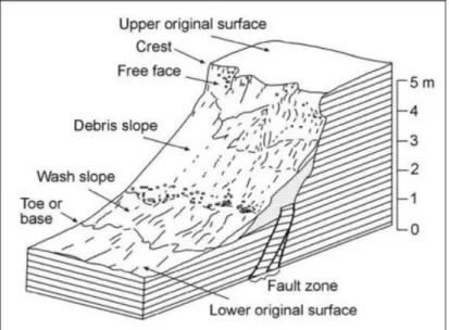
At the time scale of a single earthquake, the most obvious manifestation of active deformation at the surface are coseismic fault scarps, tectonic landforms generally coincident with a fault plane and produced almost instantaneously when an earthquake rupture propagates up to the surface. Scarp formed by normal faulting earthquakes are generally located along preexisting faults at the contact between bedrock and colluvial or alluvial deposits or can occur as fresh, steeply inclined scarps within unconsolidated sediments (figures 2.8 – 2.9). Normal fault scarps resulting from a single increment of displacement along a fault can range in height from few centimeters to more than 10 meters.
Figure 2.8 - Basic slope elements that may be present on a piedmont fault scarp (after Wallace, 1977).
Figure 2.9 - Coseismic fault scarp of the 1915 Pleasant Valley (Ms 7.7) earthquake
A more detailed description of the geomorphic characteristics of young fault scarps can be found in Wallace, 1977.
15
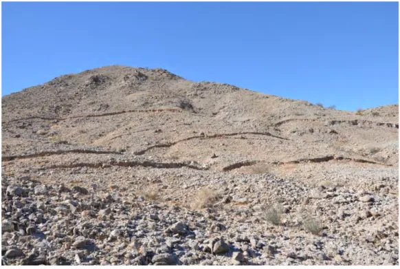
Repeated displacements along the same fault can concur to form a compound fault scarp (Slemmons, 1957), also called composite (Stewart and Hancock, 1990) or multiple-event fault scarps, as the one visible in figure 2.10.
Figure 2.10 - Compound fault scarp – Humboldt range, Nevada, USA
At a mature stage, when deformation has been cumulated for several seismic cycles, normal faulting generates a characteristic basin and range topography, common in regions of presently active extension like large parts of Nevada, Utah, Greece, western Turkey and Italy.
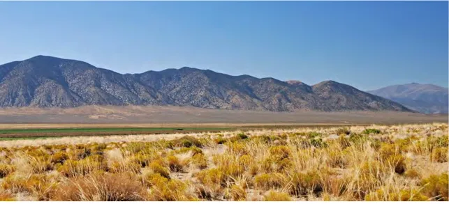
In these regions the most evident landforms are mountain fronts that represent zones of topographic transition between uplifted mountains and plains. A typical normal fault mountain front is characterized by an assemblage of landforms that includes the escarpment, the streams that dissect it and the adjacent piedmont landforms (figure 2.11).
Figure 2.11 - Stillwater range, Dixie Valley, Nevada
The cumulative displacements on a range-bounding normal fault create disequilibrium and a base-level fall that causes deep valleys (e.g. wine glasses valleys) to be carved in the relatively uplifted footwall block and favors the
16
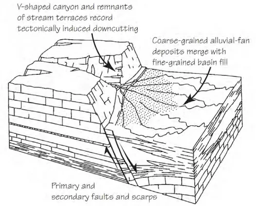
sedimentation of alluvial-fan deposits in the subsided hangingwall (figure 2.12 - modified after Keller and Pinter, 2002).
Figure 2.12 - idealized diagram showing the topographic expression of an active normal fault system (after Bull, 2007).
An ideal sequential development of a single fault-generated mountain escarpment is well depicted in figure 2.13 and may be useful to visualize some of the concepts showed before. Initial faulting creates a linear scarp (A) that later on tends to migrate away from the base of the rising range (B). At stage C, tectonically induced valleys are notched into the rising block; the occurrence of earthquakes along the same structure maintains a steep, straight mountain front (D). After cessation of uplift, or with more competitive erosional processes, the mountain front becomes sinuous and the relief starts to degrade, lowering the ridgecrests (E).
17 Figure 2.13 - block diagram showing the sequential development of a single fault-generated mountain escarpment (modified after Wallace, 1977)
2.3 Examples from the Basin and Range Province and from the Walker Lane, Nevada, USA
During the time I spent at the Center for Neoteconic Studies of the University of Nevada, Reno, I had the opportunity to visit some of the best morphological expressions of active normal faults in the western U.S.A., in particular the Humboldt Range and the Wassuk Range, located in the Basin and Range Province and the Walker Lane, respectively.
The Humboldt range is a uplifted block with important normal faults on both E-W sides (horst) composed primarily of Permo-Triassic metasedimentary and intrusive rocks (Silberling and Wallace, 1967; Wallace et al., 1969), with peaks rising to elevations of ~ 2900 m a.s.l. close to the adjacent basins laying at ~ 1300 m a.s.l.. Figure 2.14 is a large-scale view of the Humboldt Range, where the morphological expression of Quaternary displacement is greater along the western flank, with a set of range-front normal faults and series of echelon scarps along piedmont faults.
18 Figure 2.14 – Shaded relief of the Humboldt Range
Youthful and repeated movement along the range-bounding faults is expressed by offset of highstand shoreline features (figure 2.15) of pluvial Lake Lahontan (about 13 ka - Adams & Wesnousky, 1999) and by the truncation and progressively increasing offset of older alluvial fan surfaces (figure 2.16).
19 Figure 2.15 - Fault scarp truncating the highstand shoreline features of pluvial Lake Lahontan along the northern end of the fault – Humboldt Range, Nevada, USA
Figure 2.16 - Aerial view of alluvial fan surfaces showing progressively increasing offset; the older alluvial surface (on the right) is characterized by greater uplift and dissection – Humboldt Range, Nevada, USA
20
Figure 2.17 – Shaded relief view of the Wassuk Range
Moreover, the Wassuk Range is an east-tilted actively uplifting mountain block composed predominantly of granite with lesser amounts of granodiorite and metavolcanics located near the western margin of the Great Basin. The range strikes northwesterly about 90 kilometers and reaches elevations of more than 3000 m; the adjacent basin being partially filled by the Walker lake.
The overall morphology is dominated by the steep east flank, bounded by a high-angle normal fault with an abrupt sinuous trace and triangular facets, reflecting active normal faulting (figure 2.17 and 2.18).
21 Figure 2.18 - steep mountain front along a portion of the east flank of the Wassuk Range, Nevada, USA
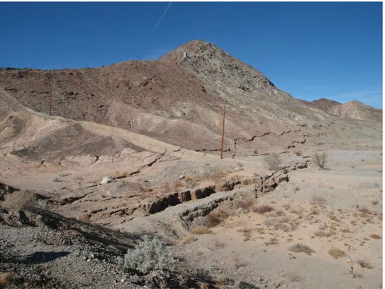
Chronological constraints of the Quaternary activity of this fault come from Late Pleistocene shorelines related to the highstand of pluvial Lake Lahontan (about 13 ka - Adams & Wesnousky, 1999), preserved along the mountain front. Holocene fault scarps are present along the entire rangefront and at the mouths of active drainages commonly reach 4 to 6 m height, (figure 2.19). Longer-term Quaternary offset is visible in 20 m to 40 m high scarps truncating older alluvial fan surfaces along the northern sector of the range (Wesnousky, 2005).
Figure 2.19 - Quaternary fault scarp in alluvial fan deposits along the northern portion of the Wassuk Range, Nevada, USA
22
2.4 Slip-rate
The main subject of this thesis is the slip-rate and the different methodologies that can concur to estimate it.
Fault slip-rate is essentially a space/time problem, which in geology translates into a displacement/age problem.
More in detail, the slip-rate represents the amount of strain that accumulates and then is released across a fault in a given time period and is defined as the ratio of slip (displacement) to the time interval over which that slip occurred.
A key fact about slip-rate to keep in mind is that it does not represent constant motion along a fault, even though the motions of tectonic plates are constant. Instead, the slip-rate represents an average of the total slip along a fault over a certain period of time.
Slip-rate is one of the fundamental descriptors of fault activity and represents a key in understanding the relative "importance" of faults in an area, as well as tectonic activity and earthquake recurrence in a region.
As a consequence, slip-rates are critical input data for assessing the seismic hazard assessment (SHA) of active fault zones. For this reason a great amount of efforts is spent trying to estimate slip-rates and discriminate between seismically active and inactive faults.
There are several ways to estimate the slip-rate of an active fault. In any case, we need a data set containing fault displacement and precise age control on deformed deposits spanning a significant portion of a fault’s life.
These data are often difficult to find, mainly because their preservation requires a delicate balance to be maintained between sedimentation, erosion, regional tectonic uplift and fault displacement through sufficiently long periods of time.
In order to obtain these data, we can use both direct and indirect approaches.
Direct approaches are those mainly related to geological disciplines, such as geology, geomorphology and tectonic, while indirect approaches are commonly related to geophysical disciplines, such as seismology, geodesy and subsurface geophysics. Depending on the type of the available information, fault slip-rates can be estimated at different spatial and temporal scales. It is possible to estimate fault slip-rates over spans of millions of years (several seismic cycles of large-magnitude earthquakes on a fault) to hundreds of years (a single seismic cycle, or a part of a cycle).
Moreover, it is possible to estimate fault slip-rates taking into account the deformation recorded by an entire range front, or using the cumulative displacement on a surface (an alluvial fan surface, i.e.) as well as analyzing a single-event displacement.
A common and direct way to estimate the slip-rate of a fault is to find a geological or morphological feature, the age of which can be determined, that has been offset by the fault being studied. A faulted paleosurface, which may contain deposits suitable to be dated, is an excellent example. Dividing the offset showed by the two portions
23
of the paleosurface by the estimated time since the paleosurface was first created (before it was cut by the fault), it is possible to estimate a slip-rate for the fault.
It is important to note that geological slip-rate rate estimates are minimum estimates, because the feature used to define fault offset formed some unknown time prior to fault initiation.
24 3 The Mw 6.3 6 April 2009 L’Aquila earthquake
The April 6, 2009 L’Aquila earthquake, with its long aftershock sequence, probably produced the largest amount of experimental data ever recorded in Italy for a single earthquake. These include seismological, geodetic, subsurface exploration and geological data.
For the purposes of this thesis, after a brief overview of the seismic sequence and of the main event, we will focus on coseismically induced deformations on the environment, with special attention to the displacement field as imaged by DInSAR and GPS and to the surface effects and ruptures detected during the geologic field survey.
3.1 Seismic sequence and causative fault
On April 6, 2009 (01:32 UTC – 03:32 Italian time), a strong earthquake (Mw6.3) struck a densely populated area in the Apennines portion of the Abruzzi region and was felt in a wide area of central Italy (figure 3.1). More than 300 people were killed and 70000 were left homeless. Although seismic hazard maps considered this area as one with the highest earthquake probability, this disaster highlighted the fragility of our historical towns and the need for a better understanding of the Italian active faults and of their seismic potential. Data recorded by permanent and temporary stations of the National Seismic Network (RSNC) managed by the Istituto Nazionale di Geofisica e Vulcanologia (INGV), by the national and local geodetic network, remote sensing and geologic data, all allowed to define the space-time evolution of the entire seismic sequence and to obtain important information on the location and geometry of the fault system responsible for the event.
25
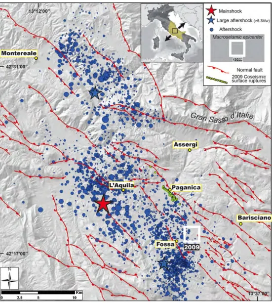
Figure 3.1 - The 2009 L’Aquila seismic sequence as recorded by the INGV Italian National Seismic Network (Chiarabba et al., 2009). Focal mechanism of the main shock and of the two largest aftershocks (Pondrelli et al., 2010) are shown (modified after Cinti et al., 2011). The macroseismic epicenter location (from damage and felt reports) of the 2009 event was computed using the Code Boxer 4.0 (Gasperini et al., 2010). The white box is the projection to the surface of the ~ 18 km-long fault modeled by Cirella et al., (2009). The white line is the expected emergence of the fault at surface. The inset in the upper right shows the direction of extension across the central Apennines (black arrows) and the regional felt area for the 6 April mainshock (colored area).
3.1.1 The Seismic sequence
The Mw 6.3 April 6, 2009 mainshock was preceded by a long seismic activity characterized by a sequence of foreshocks clustering around the main shock nucleation area. This foreshock sequencestarted in October 2008 and culminated with a Mw 4.4 event on march 30 2009 and a Mw 4.2 earthquake a few hours before the mainshock. The main shock is located just beneath the town of L’Aquila and nucleated in the upper crust at a depth of ~9.5 km.
Following the April 6 mainshock, a total area of more than 1000 km2 was interested
26 with respect to the mainshock epicenter (figure 3.1). The 2009 L’Aquila seismic sequence activated a normal fault system reaching a total length of about 50 km in the NW-trending direction. Most of the events show hypocentral depths ranging from ~15 km to ~2 km, within the typical seismogenic thickness of central Apennines. Moreover, the southern seismicity cluster was characterized by the deepest hypocentral depths, with earthquakes deeper than 20 km.
A total of seven MW ≥ 5 and numerous MW ≥ 4 aftershocks occurred during the
weeks after the mainshock, with more than 30,000 seismic events recorded during the whole sequence.
The plot in figure 3.2 shows the cumulative energy released during the 2009 L’Aquila seismic sequence (from January to July 2009). It is noticeable that the relative contribution in terms of energy related to the whole foreshock sequence is comparable to the energy released by the Mw 4.4 event of March30, while is clear that most of the energy released in the whole seismic sequence is related to the Mw 6.3 April 6, 2009 mainshock. Taking into account this information, we can expect that most of the coseismic deformation at depth and at the surface is related to the April 6 mainshock.
Figure 3.2 – Cumulative seismic energy release (joule) from January to July 2009 (after Pondrelli et al., 2010).
Looking at the focal mechanisms of the larger earthquakes, we can see that the entire seismic sequence is dominated by NE-SW oriented extension, in good agreement with geodesy and regional tectonics (figure 3.3), with only few events showing a strike-slip component (Pondrelli et al., 2010).
27
Figure 3.3 - Regional centroid moment tensors (RCMTs) with their epicenters (in red) and the smaller magnitude events of the L’Aquila 2009 seismic sequence (in yellow, Chiarabba et al. 2009). In the background (green and blue dots) previous seismicity (CSI, Castello et al. 2007) and previous available RCMTs (small focal mechanisms, Pondrelli et al. 2006; http://www.bo.ingv.it/RCMT/Italydataset.html). (Modified after http://www.bo.ingv.it/indagini-terremoto-del-06042009-in-abruzzo-laquila.html)
Although the magnitude of the mainshock is not among the largest occurred in the central Apennines in the past, the L’Aquila earthquake can be considered one of the most disastrous of the last century. The earthquake caused more than 300 deaths and left sixty thousand homeless. Severe damage was observed in the town of L’Aquila and in several villages within a radius of ~50 km. The partial or complete collapse of a significant number of old or badly maintained buildings occurred but also some reinforced concrete buildings collapsed. The very strong ground motion occurred especially close to the fault, with accelerations up to 0.63 g (Akinci et al., 2010), likely increased the damage. The effects of the shaking were recorded not only in the epicentral zone but also in distant areas like the city of Rome (~90 km from the epicenter).
The macroseismic survey performed after the main shock (Galli and Camassi 2009) shows that the largest damage is distributed in a NW-SE oriented direction, with a maximum assessed intensity of 9–10 MCS (Mercalli – Cancani - Sieberg scale) and a total of 16 localities suffering intensity larger than 8 MCS (figure 3.4).
28
Figure 3.4 – Map showing the results of the macroseismic survey. The black rectangle indicates the macroseismic box based on the distribution of macroseismic intensities. (after Galli and Camassi, 2009).
3.1.2 The earthquake causative fault: the Paganica fault
The large amount of data acquired during the sequence was used to constrain the location and the geometry of the fault system responsible for the 2009 L’Aquila mainshock. In particular the aftershocks distribution (figure 3.5), together with DInSAR analysis, body waves seismology, strong motion records and GPS observations and surface faulting all concurred to image the geometry of the fault responsible for the 6 April main shock.
Source modeling resulting from the inversion of geodetic and seismological data revealed a heterogeneous slip distribution on the fault plane (Anzidei et al., 2009; Atzori et al., 2009; Cheloni et al., 2010; Cirella et al., 2009; Pino & Di Luccio, 2009; Trasatti et al., 2011). The rupture pattern was characterized by two main slip patches: the largest slip concentration at depth was located southeastward from the hypocenter and showed a maximum slip of ~1.1 m; a second smaller patch was observed above the hypocenter and was characterized by a maximum slip of ~0.7 m. The rupture history is characterized by directivity effects, with an up-dip initial rupture propagation followed by a second rupture propagating along fault strike to the south-east (Cirella et al., 2009; Pino & Di Luccio, 2009). Slip on the fault plane is predominantly normal dip-slip (Chiarabba et al., 2009; Pondrelli et al., 2010), with a minor right-lateral component (Cirella et al., 2009; Walters et al., 2009).
All the modeling efforts (Anzidei et al., 2009; Atzori et al., 2009; Cheloni et al., 2010; Chiarabba et al., 2009; Cirella et al., 2009; Pino & Di Luccio, 2009; Trasatti et al., 2011; Walters et al., 2009) converge toward a causative fault characterized by:
29 • a NW-SE orientation;
• 15-18 km of length; • 42°- 55° dip to the SW.
Figure 3.5 – Vertical section across the Paganica Fault with aftershocks showing fault geometry.
3.2 Earthquake effects on the environment
The 2009 Mw 6.3 L’Aquila earthquake was associated with an extensive and complex set of surface coseismic deformations, involving an area of hundreds of km2.
In the following section the whole coseismic deformation pattern will be illustrated, starting from the “big picture” revealed by DInSAR and GPS analysis and then describing the most relevant surface ruptures recognized during the field survey.
3.2.1 Coseismic deformation
An important amount of information on the coseismic deformation related to the 2009 Mw 6.3 earthquake came from satellite data (DinSAR and GPS, mainly).
Differential SAR Interferometry (DInSAR) is a microwave remote sensing technique that uses the phase difference (interferogram) between two temporally separated Synthetic Aperture Radar (SAR) images of an investigated area to detect elevation
30 changes in the radar line of sight (LOS) over large areas. DInSAR is an effective technique in measuring ground deformations and provides spatially dense deformation fields with great accuracy (1 cm or less) (Gabriel et al., 1989).
After the 2009 L’Aquila earthquake several authors applied this technique to the L’Aquila area, with the aim to image the coseismic ground deformation at a large scale.
The deformation induced by the earthquake as seen by DInSAR is almost vertical and is detectable over an area of about 500 km2 extending SE from the mainshock
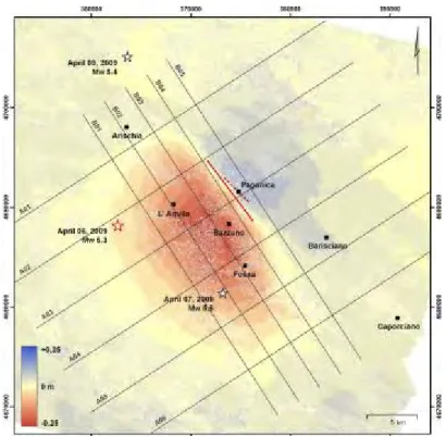
epicenter. The concentric color fringe pattern visible in the three interferograms, (figure 3.6) define the displacement field which is evident as subsiding areas (~65%) in the hangingwall of the Paganica fault and as uplifted areas (~35%) in the footwall block.
The maximum displacement (lowering) occurred between L’Aquila town and Fossa village, with values ranging from 16 to 28 cm for COSMO ascending and ENVISAT ascending and descending, respectively while the maximum footwall uplift not exceeded 10 cm (Atzori et al., 2009; Walkers et al., 2009; Papanikolaou et al., 2010; Trasatti et al., 2011).
Figure 3.6 - Differential interferograms from: (a) COSMO-SkyMed ascending, (b) Envisat ascending, (c) Envisat descending (with looking directions). The main event of the 6 April 2009 and the Paganica fault are also shown (after Atzori et al., 2009).
The spatial variability of ground deformation is highlighted by a set of cross sections drown both perpendicular and parallel to the activated fault plane (figure 3.7 - Papanikolaou et al., 2010). The abovementioned profiles revealed an asymmetric deformation pattern, with the maximum subsidence recorded near the hangingwall center (Profiles A03 and B03 in figures 3.8 and 3.9).
31
Figure 3.7 – Displacement field of the 6 and 7 April 2009 earthquakes and location of the cross-sections showing differences in the deformation field (after Papanikolaou et al., 2010).
32
Figure 3.9 – Profiles parallel to the activated fault plane (after Papanikolaou et al., 2010).
Furthermore, interesting information was derived from continuous and survey-style GPS stations located in the epicentral area of the mainshock.
The Global Positioning System (GPS) is a geodetic space technique effective in defining the relative positions of observation sites located on the Earth’s surface with centimetric precision and without the limitation of the terrestrial techniques, such as the mutual visibility between the observation sites. This technique allows to study tectonic processes both on regional and local scale and to estimate the ongoing crustal deformation within a region.
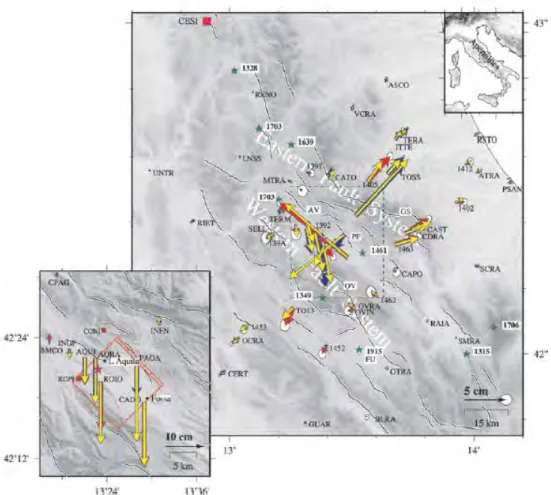
Analysis based on continuous and survey-style GPS stations that measured directly the coseismic displacement, allowed researchers estimating the deformation due to the L’Aquila earthquake (Anzidei et al., 2009; Cheloni et al., 2010) and highlighted significant horizontal and vertical permanent deformations in the epicentral area, within a radius of ~ 60 km from the mainshock (figure 3.10).
GPS sites showed clear evidence for coseismic offset, with maximum horizontal and vertical coseismic displacements of ~10 and ~ –15 cm, respectively, observed in the hangingwall of the Paganica fault, while the displacement related to the footwall motion was ~ 7 cm.
Due to the daily sampling of the GPS time-series, Cheloni et al., 2010 provided also an estimate of the afterslip occurred during the first day, that reach values between 1.0 and ~5 cm (figure 3.11).
33
Figure 3.10 - GPS coseismic displacements of the 2009 April 6th Mw 6.3 L’Aquila earthquake (pink star,
epicentre; blue vectors, continuous GPS; red, survey-style GPS; yellow, uniform slip dislocation model; error ellipses at 95 per cent C.I.; green stars, Imax > X historic earthquakes labelled with A.D. epoch). Black lines are active faults from Galli et al. (2008), Boncio et al. (2004) and Roberts & Michetti (2004). The red square indicates the position of the station CESI. The inset shows observed (blue) and calculated (yellow) vertical displacements. (after Cheloni et al., 2010)
Figure 3.11 - Time-series of PAGA and AQUI sites. The dashed line is the best-fitting exponential function. Arrows correspond to estimated coseismic offsets (red) and post-seismic cumulated displacements (blue). (after Cheloni et al., 2010)
34 3.2.2 Coseismic surface effects and ground ruptures
Immediately after the April 6 2009 mainshock and in the following weeks, a field geological survey was performed in the epicentral area by several geologists, among them the EMERGEO Working Group (INGV prompt geological survey team), in order to identify and to characterize the coseismic surface effects. During my work at the INGV, I had the opportunity to join the geological survey team and to gather observations and data regarding type, style and magnitude of the coseismic surface deformations. The data collected (about 400 sites) during the post-earthquake field campaigns evidenced a widespread and diversified set of geological surface effects (figure 3.12).
Most of the deformation at the surface was expressed as tectonic ruptures with or without throw, showing similar, if not identical strikes. These coseismic features were mostly observed on Quaternary deposits along pre-existing scarps, paralleling the Paganica fault. Other discontinuous, short, open cracks occurred along both pre-existing fault traces or on the plain and these effects may be interpreted as related mainly to triggered slip or seismic shaking. Rock falls, landslides, liquefactions, soil compactions and mobilization of loose deposits were among the other secondary surface effects observed in the epicentral area and likely related to seismic shaking and/or gravitational phenomena.
35
Figure 3.12- Map of the investigated sites for the survey of coseismic geological effects. Colors indicate sites with different types of observations: tectonic ruptures and shaking effects. The purple box includes the Paganica ruptures, which are interpreted to be primary surface faulting. We also show the sites along faults where no ruptures or other effects were observed. Stars indicate the three main events. Rose diagrams of the tectonic surface ruptures: (A) total data; (B) Paganica fault; (C) Mt. Bazzano fault and (D) Monticchio-Fossa fault. We do not report rose diagrams when the data are less than five measurements.
The observed coseismic ground effects in the epicentral area were arranged in a typical pattern for a M~6 earthquake, as described by the idealized schematic block-diagram of figure 3.13 (Dramis & Blumetti, 2005).
36
Figure 3.13 – Schematic block-diagram of a Quaternary intramontane basin associated with a ≅M 6 earthquake. Typical seismo-tectonic and seismo-gravitational landforms related to the repetition of coseismic effects along the same seismogenic structure. 1) primary surface ruptures; 2) secondary and sympathetic surface ruptures; 3) deep-seated gravitational deformation; 4) landslide; 5) ground failure; 6) liquefaction. (after Dramis and Blumetti, 2005).
Among all the surveyed coseismic effects, the most prominent tectonic ruptures were observed in the east side of the Middle Aterno Valley, along a portion of the NW-trending, SW-dipping Paganica normal fault system. Here the surface ruptures can be observed with a clear expression for a continuous extent of ~3 km in coincidence with the long-term morphological expression of the fault and are usually confined within ~30 m from the fault scarp (figure 3.14).
37
Figure 3.14 - Detail of the area of the 3 km long continuous surface ruptures along the escarpment bounding the Paganica village. Topographic color ramp derived from a 5 m resolution DEM. Contour lines interval is 25 m. (modified after Cinti et al., 2011)
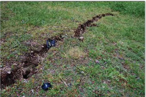
The main characteristics of the surface ruptures along the Paganica fault are: • mostly open cracks (maximum opening ~10 cm) – figure 3.16;
• vertical dislocations or flexural scarps with a maximum vertical throw of 15 cm (southwest-side down) – figure 3.15;
• the alignment of the ruptures shows a clear spatial continuity and persistent orientation of N130° - N140°;
• commonly organized in en-echelon arrangement;
• occur regardless of slope angle, the type of deposits crossed or the type of manmade feature, and thus independently from gravitational effects.
38
Figure 3.15 - Surface rupture along the Paganica fault with a maximum throw of 15 cm.
Figure 3.16 - Surface rupture along the Paganica fault with a maximum opening of 10 cm and a negligible throw.
Despite maximum vertical throws not exceeding 15 cm, the location, continuity and the consistency of the surface ruptures along the Paganica fault where not observed along any other structure within the epicentral area.
39 Both to the north and to the south of this ~ 3 km continuous section, the surface ruptures fade out and discontinuous open fissures occurred along similar trends. Depending on whether or not these discontinuous fissures are interpreted as evidence of coseismic slip on the Paganica Fault at depth, different interpretation report the length of the 6 April 2009 primary surface faulting between 3 and 19 km (Falcucci et al., 2009; Boncio et al., 2010; Emergeo Working Group, 2010; Galli et al., 2010, Vittori et al., 2011).
3.3 Summary
Summarizing, both DInSAR and GPS dataset analysis revealed the amount and spatial extent of the coseismic deformation field and allowed to model the source parameters and the slip distribution on the fault plane (Atzori et al., 2009; Cirella et al., 2009; Cheloni et al., 2010; Walters et al., 2009, Papanikoalou, 2010).
The location of the 3 km-long surface faulting zone observed during the field campaign coincides with the zone of maximum coseismic slip at depth imaged through the joint inversion of GPS and strong motion data (Cirella et al., 2009).
Moreover, the aftershocks distribution, the focal plane solutions, the geometry and kinematics of the 2009 surface ruptures along the Paganica fault and the whole coseismic displacement field are all consistent with the long-term trace of the PF. In fact, the coseismically uplifted areas coincide with the footwall block of the PF while the subsiding areas with the basin in the active hangingwall (figure 3.17).
40
Figure 3.17 - The coloured contour fringes define the displacement field from the ENVISAT differential Interferogram. The maximum lowering is ca. 0.28 m N of Monticchio. Green dots represent continuous coseismic surface ruptures, light blue triangles are discontinuous open fissures.
Taking into account all these observations, there is evidence that the Mw 6.3 April 6, 2009 earthquake occurred on the previously mapped NW-SE, SW-dipping Paganica fault (Bagnaia et al., 1992; Vezzani and Ghisetti, 1998; Boncio et al., 2004; Geological Map of Italy, scale 1:50.000, sheet 359, L’Aquila, APAT, 2006).
A detailed description of the field geological survey and of the observations of the surface geological effects in the epicentral area is available in the attached Terra Nova article “Evidence for surface rupture associated with the Mw 6.3 L’Aquila earthquake sequence of April 2009 (Central Italy)” which I co-authored.
From now on, we will refer to the 2009 earthquake causative fault as the Paganica – San Demetrio fault system (PSDFS herein) after, also according to the work of Bagnaia et al., 1992.