hyperfine coupling constants in solution
by a QM/MM approach: Interplay between
electrostatics and non-electrostatic effects
Cite as: J. Chem. Phys. 150, 124102 (2019); https://doi.org/10.1063/1.5080810Submitted: 12 November 2018 . Accepted: 25 February 2019 . Published Online: 25 March 2019 Tommaso Giovannini , Piero Lafiosca, Balasubramanian Chandramouli , Vincenzo Barone , and Chiara Cappelli
ARTICLES YOU MAY BE INTERESTED IN
Perspective: Computational chemistry software and its advancement as illustrated through
three grand challenge cases for molecular science
The Journal of Chemical Physics
149, 180901 (2018);
https://doi.org/10.1063/1.5052551
Ab initio quantum mechanics/molecular mechanics method with periodic boundaries
employing Ewald summation technique to electron-charge interaction: Treatment of the
surface-dipole term
The Journal of Chemical Physics
150, 124103 (2019);
https://doi.org/10.1063/1.5048451
An extension of the fewest switches surface hopping algorithm to complex Hamiltonians
and photophysics in magnetic fields: Berry curvature and “magnetic” forces
Effective yet reliable computation of hyperfine
coupling constants in solution by a QM/MM
approach: Interplay between electrostatics
and non-electrostatic effects
Cite as: J. Chem. Phys. 150, 124102 (2019);doi: 10.1063/1.5080810
Submitted: 12 November 2018 • Accepted: 25 February 2019 • Published Online: 25 March 2019
Tommaso Giovannini,1,a) Piero Lafiosca,1 Balasubramanian Chandramouli,1,2 Vincenzo Barone,1
and Chiara Cappelli1,b)
AFFILIATIONS
1Scuola Normale Superiore, Piazza dei Cavalieri 7, 56126 Pisa, Italy
2Compunet, Istituto Italiano di Tecnologia (IIT), Via Morego 30, 16163 Genova, Italy a)
Electronic mail:[email protected] b)Electronic mail:[email protected]
ABSTRACT
In this paper, we have extended to the calculation of hyperfine coupling constants, the model recently proposed by some of the present authors [Giovannini et al., J. Chem. Theory Comput. 13, 4854–4870 (2017)] to include Pauli repulsion and dispersion effects in Quantum Mechan-ical/Molecular Mechanics (QM/MM) approaches. The peculiarity of the proposed approach stands in the fact that repulsion/dispersion contributions are explicitly introduced in the QM Hamiltonian. Therefore, such terms not only enter the evaluation of energetic proper-ties but also propagate to molecular properproper-ties and spectra. A novel parametrization of the electrostatic fluctuating charge force field has been developed, thus allowing a quantitative reproduction of reference QM interaction energies. Such a parametrization has been then tested against the prediction of EPR parameters of prototypical nitroxide radicals in aqueous solutions.
Published under license by AIP Publishing.https://doi.org/10.1063/1.5080810
I. INTRODUCTION
In the last decades, multiscale models have been widely used for the study of molecular properties and spectra.1–11 In this
con-text, the most successful approaches fall within the class of “focused models,” which aim at accurately modeling both the physico-chemical properties of the target and its interactions with the surrounding environment. The effect of the latter is seen as a per-turbation on the target molecule and is treated at a lower com-putational level of theory, e.g., by resorting to classical physics, whereas the target molecule is described accurately, generally at the Quantum Mechanical (QM) level. Due to such a partitioning, the computational cost of a QM/classical computation is compara-ble to that of the corresponding QM isolated system. Such a fea-ture has strongly contributed to the increasing popularity of these models.
QM/Molecular Mechanics (MM) models are among the most renowned classes of QM/classical approaches,2,12–18 which have
been formalized within different physical frameworks. Beyond the basic mechanical QM/MM embedding, in the last years, much effort has been spent to define electrostatic QM/MM embedding approaches, in which a set of fixed charges is placed on the MM moi-ety (generally on MM atoms), and the interaction between QM and MM portions is modeled by resorting to the Coulomb law. Clearly, in such approaches, the QM and MM moieties do not mutually polarize. Mutual polarization, i.e., the polarization of the MM por-tion arising from the interacpor-tion with the QM density and vice versa, can be introduced by employing polarizable force-fields, which can be based on distributed multipoles,19–23induced dipoles,24–26
Drude oscillators,27or Fluctuating Charges (FQs).8,28,29
The description of the molecular properties/spectra of embed-ded systems which is obtained by resorting to polarizable embedding
is generally quite accurate.22,25,26,30–32 However, such models are
deeply based on the assumption that electrostatic energy terms dom-inate the target/environment interactions. Non-electrostatic (Pauli repulsion and dispersion) contributions between the QM and MM portions are roughly modeled by using parametrized functions, e.g., the Lennard-Jones potential,33,34 which are however completely
independent of the QM density. As a result, they are not taken into account in the QM operators so that the calculated spectro-scopic/response properties are not affected by such interactions. The reasons why such contributions are generally discarded are connected to the presumption of a numerically dominating effect of electrostatic terms. However, non-electrostatic contributions are crucial to get a physically consistent description of any embed-ded system, also in the case of target/environment interactions dominated by electrostatics.35,36
A way to include non-electrostatic energy terms is to resort to the Effective Fragment Potential (EFP).19,20,37–40The high
accu-racy of this method is essentially due to the explicit QM calcula-tion of the molecular orbitals of the environment, drifting apart from the concept at the basis of MM Force Field (FF). A simi-lar QM-based approach, namely, the Posimi-larizable Density Embed-ding (PDE), has been recently proposed to only include repulsion effects.41,42
A substantially different way of including non-electrostatic interactions in QM/MM approaches consists of exploiting a model recently developed by some of the present authors,43which
formu-lates repulsion as a function of an auxiliary density on the MM por-tion and extends the Tkatchenko-Scheffler (TS) approach to density functional theory (DFT)44–48 to treat QM/MM dispersion terms.
Notice that the formulation of repulsion contributions in terms of gaussian functions placed in the MM region has also been pro-posed in the so-called Gaussian Electrostatic Model (GEM).36,49–51
However, in both the aforementioned PDE and GEM models, repul-sion interaction is modeled as an overlap one-electron integral. Our approach instead defines repulsion contributions in terms of a two-electron exchange integral, thus physically representing the Pauli repulsion. Moreover, differently from the stand-alone approaches discussed above (EFP, PDE, GEM), our approach can easily be cou-pled to any kind of QM/MM approach because repulsion and dis-persion are formulated in a way which is totally independent of the choice of the FF to model the electrostatics (i.e., fixed-charges or polarizable embedding). Remarkably, in our model, repulsion and dispersion contributions are indeed dependent on the QM density. Thus, an explicit contribution to the QM Fock operator exists and the resulting calculated QM properties/spectra are modified by such interactions.
Our model for non-electrostatics in QM/MM has been so far only challenged on reproducing full QM non-electrostatic interac-tion energies, for which very good results have been obtained.43
In this paper, we start with the extension of the model to spec-troscopy. To this end, we report the formulation of non-electrostatic QM/MM terms for EPR, for which environmental effects substan-tially contribute to the overall observable.52–54Environmental
(sol-vent) effects on EPR are usually described by means of continuum models55–58and only in few cases by adopting electrostatic QM/MM
embedding coupled with a classical Molecular Dynamics (MD) to take into account the fluctuations of both the solute conformations and the solvent molecules.59–65
Nitroxide radicals are among the most thoroughly studied rad-icals from both experimental and computational points of view due to their remarkable stability coupled to strong sensitivity to the polarity of the surrounding and to the pyramidality of the nitro-gen atom. Given their importance, several nitroxide radicals have been synthesized to be either used as spin probes (when dispersed in an environment) or as spin labels (when chemically attached to a biological molecule, e.g., a protein).66–68 High-field EPR
spec-troscopy provides quite rich information consisting essentially of the nitrogen hyperfine and gyromagnetic tensors.66However,
interpre-tation of these experiments in structural terms strongly benefits from quantum mechanical calculations able to dissect the overall observ-ables in terms of the interplay of several subtle effects.59,60,69–75
This situation has prompted us to perform a comprehensive study of prototypical nitroxide radicals in aqueous solution coupling den-sity functional and coupled cluster quantum mechanical computa-tions to molecular dynamics simulacomputa-tions, and average of properties for a sufficient number of snapshots including electrostatic, induc-tion, repulsion, and dispersion interactions with the surrounding evaluated by effective quantum mechanical approximations.
To the best of our knowledge, this work presents the first for-mulation and application of a QM/MM approach accounting at the same time for polarization and non-electrostatic interactions on EPR Hyperfine Coupling Constant (hcc).
The paper is organized as follows: first, the theoretical model is presented. Then, the computational approach is applied to the cal-culation of hccNof two nitroxyl radicals (PROXYL and TEMPO) in
aqueous solution. Such compounds are characterized by the pres-ence of the N–O group, which has been most widely used as “spin probe” and “spin label” for the study of structure and dynamics of macromolecular systems.66–68Summary and Conclusions end the
manuscript.
II. THEORETICAL MODEL
The total energy of a system composed by two interacting moi-eties, one described at the QM level and the other at the MM level, can be expressed as76,77 EQM/MM= E ele QM/MM+ E pol QM/MM+ E ex−rep QM/MM+ E dis QM/MM, (1)
where EeleQM/MM accounts for electrostatic interactions and EpolQM/MM is the polarization contribution. Such energy terms are those mod-eled in the electrostatic embedding approach and, in particular, in polarizable QM/MM methods.2,12,24–27,78Eex−rep
QM/MMis the
exchange-repulsion contribution and EdisQM/MMarises from dispersion interac-tions.
In this work, electrostatic and polarization terms are mod-elled by exploiting the Fluctuating Charge (FQ) force field,8,30,78–82
whereas non-electrostatic interactions (i.e., the sum of Eex−repQM/MMand EdisQM/MM) are modeled by using the model described in Ref.43. In
the next paragraphs, the mathematical formulation of the different energy contributions is discussed.
A. Electrostatic and polarization interactions
In order to model electrostatic and polarization terms [see Eq.(1)], a polarizable QM/MM embedding needs to be adopted.
In such a model, the MM force field adapts to the exter-nal field/potential originating from the QM density and electro-static/polarization terms are included in the QM Hamiltonian, so as to describe the mutual interaction between the QM density and the environment.
In this work, we will resort to the FQ force field.8In the
result-ing QM/FQ model, the electrostatic potential due to the QM density together with the differences in electronegativities between different atoms in the MM region gives rise to a charge fluctuation in the MM region, up to the point that the differences in electrochemical poten-tial between the MM atoms vanish. From a mathematical point of view, this results in the following linear equation:83
Dqλ= −CQ− V(PQM), (2)
where D is a response matrix, whose diagonal terms are atomic chemical hardnesses and q is a vector containing the FQs and Lagrangian multipliers. C contains atomic electronegativities and those constraints which are needed to ensure each MM molecule has a fixed charge. V(P) is the potential due to the QM density matrix P calculated at MM charges positions. We refer the reader to Ref.84
for further details.
The interaction between FQ charges and the QM density obeys the Coulomb law,
EQM/MMele + EQM/MMpol = NFQs ∑ j=1R∫3 ρQM(r)qj ∣r − rj∣ dr. (3)
By differentiating Eq.(3)with respect to the density matrix, Pµν,
the contribution to the Fock matrix is obtained,83
Fµν= ∂E
∂Pµν = V
†
µνq. (4)
The Fock matrix defined in this way can enter a SCF proce-dure, so as to finally give a QM density mutually equilibrated with the FQs.
B. Pauli repulsion energy
The exchange-repulsion energy, Eex−repQM/MM, also known as Pauli repulsion energy, is formally due to the Pauli principle, i.e., wave-function antisymmetry. From a mathematical point of view, it can be formulated as the opposite of an exchange integral,77,85
Eex−repQM/MM=1 2 ∫
dr1dr2
r12
ρQM(r1, r2)ρMM(r2, r1). (5)
In order to define the density matrix ρMM, we localize
ficti-tious valence electron pairs for MM molecules in bond and lone pair regions and represent them by s-gaussian-type functions. The expression for ρMMbecomes
ρMM(r1, r2) = ∑ R
ξ2Re
−βR(r1−R)2⋅ e−βR(r2−R)2, (6)
where R collects the centers of the gaussian functions used to repre-sent the fictitious MM electrons. The β and ξ parameters are gener-ally different for lone-pairs or bond-pairs, their values being adjusted
to the specific kind of environment (MM portion) to be modeled. By substituting Eq.(6)in Eq.(5), the QM/MM repulsion energy reads ErepQM/MM=1 2 ∑R ∫ dr1dr2 r12 ρQM(r1, r2) ⋅ [ξ2Re −βR(r1−R)2⋅ e−βR(r2−R)2]. (7) It is worth noticing that in this formalism, QM/MM Pauli repulsion energy is calculated as a two-electron integral. Equa-tion(7)is general enough to hold for any kind of MM environment (solvents, proteins, surfaces, etc.). The nature of the external envi-ronments is specified by defining the number of different electron-pair types and the corresponding β and ξ parameters in Eq.(6). Also, the formalism is general so that it can be coupled to any kind of QM/MM approach.
By differentiating Eq.(7)with respect to the density matrix, the corresponding contribution to the Fock matrix is obtained,
Fµνrep= ∂Erep ∂Pµν = 1 2 ∫ dr1[ χµ(r1)Aν(r1) + Aµ(r1)χν(r1) 2 ], (8)
where χµare atomic basis functions and Aµare calculated as detailed
in Ref.43.
C. Quantum dispersion energy
To formulate dispersion interactions, we start from the Tkatchenko and Scheffler (TS) DFT functional. In this model, the dispersion energy can be written as
Edis= −1 2 ∑A,B
fdamp(RAB, R0A, R0B)C6ABR−6AB, (9)
where RABis the distance between atoms A and B in a given system,
C6ABis the corresponding C6coefficient, R0Aand R0Bare their van der
Waals (vdW) radii. The R−6ABsingularity at small distances is
elimi-nated by the short-range damping function fdamp(RAB, R0A, R0B).44
C6AB coefficients can be expressed in terms of homonuclear
parameters C6AA, C6BB, which in turn can be obtained through
an Hirshfeld86 partition of the density.44 Notice that alternative
partitioning approaches can in principle be exploited.87
Such an approach can be reformulated within a QM/MM formalism,43,48yielding EdisQM/MM= − 1 2 ∑A∈QMB∈MM∑ fdamp(RAB, R 0 A, R0B) ⋅ η2ACAAfreeC eff 6BB α0 B α0 Aη 2 AC free AA+ α0 A α0 BC eff 6BB R−6AB, (10)
where Ceff6BBare effective homonuclear coefficients of B (MM) atoms and C6AAfree are free homonuclear coefficients of A QM atoms. α0Aand
α0Bare static dipole polarizabilities, whereas ηAis a function
convert-ing Cfree6AAinto Ceff6AA. Further details can be found in Refs.43,44, and
48.
fdamp(RAB, R0A, R0B) in Eq.(10)is a Fermi-type damping
fdamp(RAB, R0A, R0B) =
1 1 + exp[−d( RAB
sRR0AB − 1)]
, (11)
where R0AB= R0A+ R0B, and d and sRare free parameters.
Similarly to what has already been done for electrostatic and repulsion contributions, by differentiating Eq.(10)with respect to the QM density matrix, the dispersion contribution to the Fock matrix is obtained,43 Fµνdis= − 1 2 ∑A∈QMB∈MM∑ fdamp(RAB) ⋅ 2α0A α0 BC 2 6BBCfree6AA2ηA (α0 B α0 A Ceff6AA+α0A α0 B C6BB) 2η ρ A,µνR −6 AB. (12) The complete derivation and definition of ηρA,µνcan be found in Ref.43.
D. Hyperfine coupling constant
The spin Hamiltonian describing the interaction between the electron spin (S) of a free radical containing a magnetic nucleus of spin I and an external magnetic field (B) can be written as
HS= µB⃗S ⋅ g ⋅ ⃗B + 1̷hγ I⃗S ⋅ A ⋅ ⃗µI
, (13)
where the first term is the Zeeman interaction between the electron spin and the external magnetic field through the Bohr magneton µB
and g = ge13+ ∆gcorr. ∆gcorraccounts for the correction to the free
electron value (ge= 2.0022319) due to several terms including the
relativistic mass (∆gRM), the gauge first-order corrections (∆gC), and
a term arising from the coupling of the orbital Zeeman (OZ) and the spin–orbit coupling (SOC) operator.90,91 The second term on the
rhs of Eq.(13)describes the hyperfine interaction between S and the nuclear spin I through the hyperfine coupling tensor A. The latter, which is defined for each nucleus X, can be decomposed into two terms,
A(X) = AX13+ Adip(X). (14)
The dipolar term Adip(X) is a zero-trace tensor, whose
contri-bution vanishes in isotropic media (e.g., solutions). The first term AX(Fermi-contact interaction), which is an isotropic contribution,
is also known as hyperfine coupling constant (hcc). It is related to the spin density (ρX) at nucleus X by the following relation:
AX=
4π
3 µBµXgegX⟨SZ⟩
−1
ρα−βX , (15)
where ρα−βX can be obtained as ρα−βX = ∑
µν
Pµνα−β⟨χµ(r)∣δ(r − rX)∣χν(r)⟩. (16)
Pα−β is the difference between α and β density matrices. Because in our approach both electrostatic and non-electrostatic dis-persion/repulsion interactions enter the definition of the QM Fock operators [see Eqs. (4), (8), and (12)], Pα−β is modified. There-fore, hyperfine coupling constants with the account of electrostatic, polarization, dispersion, and repulsion QM/MM interactions are obtained.
III. COMPUTATIONAL DETAILS
Molecular geometries of PROXYL and TEMPO radicals (Fig. 1) were optimized in vacuo by combining B3LYP and PBE0 hybrid density functionals with both aug-cc-pVDZ and 6-311++G(3df,2pd) basis sets. For all optimized structures, the hyperfine coupling con-stant of nitrogen atom was calculated by exploiting both B3LYP and PBE0 and the N07D basis set.92,93 For the sake of
compari-son, on the reduced structures depicted inFig. 1, which are obtained by removing ring atoms for both TEMPO and PROXYL but keep-ing fixed all the geometrical parameters, additional coupled-cluster single double (CCSD)/EPR-II94calculations were performed.
Clusters made of TEMPO and PROXYL radicals with two explicit water molecules (seeFig. 3) were optimized at the PBE0/6-311++G(3df,2pd) level, according to previous studies.57For those
structures, the interaction energy between the radicals and the two water molecules was computed by exploiting SAPT0/aug-cc-pVTZ or jun-ccp-pVDZ or N07D (as implemented in Psi4 1.195)
and CCSD(T)/aug-cc-pVTZ, jun-cc-pVDZ, and N07D. Counter-poise corrections were included in CCSD(T) calculations. QM/MM energy calculations were also performed at the PBE0/aug-cc-pVTZ, jun-cc-pVDZ, and PBE0/N07D level, by including disper-sion and repuldisper-sion energies obtained by exploiting our model.43
The QM portion was restricted to the radical, whereas the two water molecules were treated at the MM level. The MM region was described by means of a non-polarizable force field (TIP3P96)
and the polarizable FQ approach8,78 by exploiting two literature
parametrizations28,97and a new parametrization proposed in this
work. The parameters used for modeling dispersion and repulsion interactions were taken from Ref.43. On the same structures, full QM and QM/MM nitrogen hyperfine coupling constants were cal-culated by exploiting the PBE0/N07D level of theory for treating the QM portion. For the sake of comparison, on the reduced cluster structures depicted inFig. 3, which are obtained by removing ring
FIG. 1. Top: PROXYL and TEMPO structures. Bottom: reduced structures used for
atoms for both TEMPO and PROXYL but keeping fixed all the geo-metrical parameters, additional CCSD/EPR-II94 hcc
N calculations
were performed.
Classical MD simulations were performed with the Amber soft-ware (v.12) using the ff99SB force field.98,99Parameters for
nitrox-ides were obtained from a previous study by one of the present authors.59The nitroxides were embedded in a cubic box of TIP3P
water molecules, which extended to 30 Å from the solute surface. The starting systems were equilibrated following a multistep pro-tocol: (i) minimization of the whole system for 10 000 steps, (ii) heating of the system from 103 to 303 K in 100 ps with a mild restraint of 0.5 kcal/mol Å2on the solute, and (iii) equilibration in NPT ensemble at a pressure of 1 bar and 303 K for 100 ps. The production phase was then initiated in NVT ensemble and continued for 10 ns. The simulation conditions involved Periodic Boundary Condition (PBC), a 1 fs time step for numerical inte-gration, using SHAKE for constraining bonds involving hydrogen atoms,100a 10 Å cut-off for non-bonded interactions, particle mesh
ewald (PME) for evaluating the long-range electrostatics,101
tem-perature regulation with Langevin coupling using a collision fre-quency of 1.0 ps−1, and snapshot collection in the trajectory at 1 ps interval.
A total of 200 uncorrelated snapshots were extracted from the MDs (one snapshot every 50 ps). For each snapshot, a 13 Å sphere centered at the solute’s geometric center was cut. All hyperfine cou-pling constants were calculated within the QM/FQ or QM/TIP3P framework at the PBE0/N07D level. The FQ water molecules were modeled both with the SPC FQ parameters,28 the
parametriza-tion proposed by some of the present authors,97 and the
param-eters proposed in this work. The convergence of the hccN values
with increasing number of representative snapshots was checked for both radicals. Dispersion and repulsion contributions to hccN
were included by exploiting what has been explained in Secs.II B
andII C. All QM/FQ calculations were performed by using a locally modified version of Gaussian 16.102Finally, the calculated values
were compared with the experimental data taken from Refs.103
and104.
IV. NUMERICAL RESULTS
In this section, we will report the results issuing from the appli-cation of the developed methodology to the calculation of the nitro-gen hyperfine coupling constant (hccN) of PROXYL and TEMPO
radicals in aqueous solution. In order to evaluate the role of the dif-ferent terms (electrostatic/polarization/dispersion/repulsion) con-curring with the overall solvent effect, we will present the results obtained by exploiting a hierarchy of different approaches, start-ing from a simple cluster model (isolated radical plus two water molecules) to averaging over a set of representative structures extracted from MD runs, with or without the inclusion of polar-ization/dispersion/repulsion solvent contributions. In addition, to allow a direct comparison with experimental hccN, reference values
for the isolated radicals are discussed. A. hccN of isolated radicals
PROXYL and TEMPO geometries (see Fig. 1) were opti-mized in vacuo at different levels of theory. In particular, B3LYP
and PBE0 functionals in combination with aug-cc-pVDZ (BS1) or 6-311++G(3df,2pd) (BS2) basis sets were employed. Selected geometrical parameters are reported inTable I. In particular, the N-O distance, the CαNCα angle, and the improper dihedral angle
CαNOCα were taken into consideration (seeFig. 1for atom
label-ing). Additional data obtained with B3LYP-D3 and PBE0-D3 func-tionals88can be found in Table S1 given assupplementary material.
Geometries were also optimized by exploiting the B2PLYP dou-ble hybrid functional combined with the maug-cc-pVTZ-d(H) basis set (BS3), which has been reported to reliably describe molecular geometries.105 The values reported in Table I clearly show that
B3LYP/aug-cc-pVDZ and B2PLYP/maug-cc-pVTZ-d(H) perform in a similar way. However, all the considered combinations of func-tional and basis set do not differ much from the best calculated struc-ture of both radicals. It is worth pointing out that the most relevant difference between PROXYL and TEMPO stands in the value of the improper dihedral angle CαNOCα, which is related to the nitrogen
atom pyramidalization. In fact, the angle is almost zero for PROXYL and about−21○
for TEMPO.
For all the optimized structures obtained with PBE0 and B3LYP functionals in conjunction with BS1 and BS2, hccNwere calculated
by exploiting either PBE0 or B3LYP and the N07D basis sets pur-posely parametrized for both functionals (see Refs.92and93for more details). For the sake of comparison, additional hccN
calcu-lations were performed at the CCSD/EPR-II94level on the reduced
structures depicted at the bottom ofFig. 1. All results are reported in
Table II.
hccNfor the two radicals differ by about 3 gauss at all levels.
Such differences are essentially due to the different pyramidalization of the nitroxyl group. The small discrepancies which are reported for the various optimized structures are due to small fluctuations in the improper dihedral angle (seeTable I). Notice that all calculated DFT hccNare underestimated with respect to CCSD/EPR-II values.
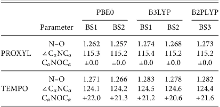
To further investigate on the role of nitrogen pyramidalization on hccN, PBE0/N07D hccNvalues for the reduced TEMPO structure
as a function of CαNOCαwere calculated. The data are graphically
reported inFig. 2.
As it can be noticed, the value computed for PROXYL and TEMPO radicals is almost recovered at zero and±20○
, respectively. For larger CαNOCαvalues, computed hccNvalues increase up to the
maximum value (22 gauss) at about±40○. Such a trend confirms
TABLE I. Selected geometrical parameters of PROXYL and TEMPO radicals at the different levels of theory. BS1: aug-cc-pVDZ; BS2: 6-311++G(3dp,2pd); BS3: maug-cc-pVTZ-d(H).
PBE0 B3LYP B2PLYP
Parameter BS1 BS2 BS1 BS2 BS3 PROXYL N–O 1.262 1.257 1.274 1.268 1.273 ∠CαNCα 115.3 115.2 115.4 115.2 115.2 CαNOCα ±0.0 ±0.0 ±0.0 ±0.0 ±0.0 TEMPO N–O 1.271 1.266 1.283 1.278 1.282 ∠CαNCα 124.1 124.2 124.5 124.6 124.4 CαNOCα ±22.0 ±21.3 ±21.2 ±20.6 ±21.6
TABLE II. Calculated hccN values (Gauss). BS1: aug-cc-pVDZ; BS2:
6-311++G(3dp,2pd).
Optimized
Radical structure PBE0/N07D B3LYP/N07D CCSD/EPR-II
PROXYL B3LYP/BS1 11.8 11.4 12.7 B3LYP/BS2 12.0 11.3 12.6 PBE0/BS1 11.8 11.1 12.4 PBE0/BS2 11.7 11.0 12.3 TEMPO B3LYP/BS1 15.0 14.4 15.9 B3LYP/BS2 14.8 14.2 15.7 PBE0/BS1 14.9 14.3 15.7 PBE0/BS2 14.7 14.0 15.4
what has already been reported by one of the present authors.60
In Fig. S1 of thesupplementary material, we report for comparison CCSD/EPR-II hccn values as a function of CαNOCα. DFT
underes-timates spin polarization (which is the only relevant contribution for the planar structure) and at the same time overestimates the singly occupied molecular orbital (SOMO) delocalization, which instead increases as the CαNOCαincreases.
B. hccN of PROXYL/TEMPO+water clusters
The most basic method to describe hydrated radicals is to resort to a cluster approach. In particular, due to the presence of the oxygen atom, a natural choice consists of saturating oxygen doublets with two water molecules (seeFig. 3).57,60According to what has already
been proposed in previous studies, all structures were optimized at the PBE0/6-311++G(3df,2pd) level.57,59
To quantify the different contributions to the radical/water interaction energy, Energy Decomposition Analysis (EDA) as for-mulated in the Symmetry-Adapted Perturbation Theory (SAPT0)106,107was performed by exploiting the aug-cc-pVTZ basis
set on the reduced structure of the PROXYL cluster (seeFig. 3).
FIG. 2. PBE0/N07D hccNvalues (Gauss) on the reduced TEMPO structure as a
function of the out of plane CαNOCαangle.
FIG. 3. PBE0/6-311++G(3df,2pd) optimized structures of clusters of PROXYL (top)
and TEMPO (bottom) with two water molecules.
Additional SAPT0 calculations were performed by exploiting both the jun-cc-pVDZ and N07D basis sets (see Table S2 given as sup-plementary material). Such additional sets were selected because jun-cc-pVDZ has been reported to provide good results for closed shell systems,108whereas N07D is exploited in this study to calculate
hccN.
SAPT0/aug-cc-pVTZ results are reported inTable III, together with the corresponding values obtained by treating the radical at the QM level (PBE0/aug-cc-pVTZ) and the two water molecules at the MM level. QM/MM electrostatic interactions were described by
TABLE III. PROXYL+2w EDA obtained by exploiting PBE0/FQ with different parametrizations and SAPT0. CCSD(T) calculations include counterpoise corrections. All data are reported in mHartree and were obtained by using the aug-cc-pVTZ basis set. FQa FQb FQc SAPT0 CCSD(T) Electrostatic −20.60 −26.80 −47.06 −31.35 ⋯ Induction ⋯ ⋯ ⋯ −11.45 ⋯ Repulsion 27.78 28.58 30.99 28.34 ⋯ Dispersion −3.28 −3.28 −3.28 −9.43 ⋯ Total 3.90 −1.50 −19.35 −23.89 −20.62 a
FQ parametrization taken from Ref.28.
bFQ parametrization taken from Ref.97. c
TABLE IV. hccNof PROXYL/TEMPO+2w clusters obtained at different levels of theory. All data are reported in gauss.
PBE0/N07D CCSD/EPR-II ∆CC/PBE0 Expt.
Electrostatic + Dispersion/
Electrostatic Repulsion
TIP3P FQa FQb FQc TIP3P FQa FQb FQc Full-QM Full-QM(red) Full-QM(red)
PROXYL 13.4 13.1 13.4 14.3 13.1 12.8 13.1 13.9 13.7 13.7 14.6 0.9 16.4
TEMPO 17.9 15.3 15.7 16.7 16.9 14.8 15.1 16.1 15.9 16.3 17.1 0.8 17.3
aFQ parametrization taken from Ref.28. b
FQ parametrization taken from Ref.97.
cFQ parametrization proposed in this work
using the FQ approach with three different parametrizations (see Table S3 in thesupplementary material), whereas QM/MM repul-sion and disperrepul-sion contributions were modeled as reported above. Additional CCSD(T)/aug-cc-pVTZ calculations including counter-poise109corrections were also performed to quantify the accuracy of
SAPT0 interaction energies.
SAPT0 values show that electrostatic interactions (i.e., the sum of electrostatic and induction terms) give larger contributions with respect to non-electrostatic (repulsion+dispersion). However, non-electrostatic interactions and in particular repulsion cannot be neglected, as it is commonly done in standard QM/MM models.
Moving to QM/FQ, we first notice that the available parametrizations (FQa and FQb inTable III) focus on modeling electrostatic interactions; however, they can indeed be inadequate whenever non-electrostatic terms are taken into consideration. This is confirmed by our results (Table III): FQa and FQb electro-static energies give a qualitatively correct description of SAPT0 or CCSD(T) total interaction energies. On the contrary, FQaand FQb total interaction energies are unsatisfactory; therefore, a novel FQ parametrization is required (labeled FQc inTable III). Differently from FQaand FQb, which were obtained to reproduce water bulk properties (FQa, Ref.28) or QM atomic charges (FQb, Ref.97), FQc is tuned to the total interaction energy at the CCSD(T) level (with an error of less than 1 kcal/mol). FQcyields an accurate description of SAPT0 electrostatic interactions. Notice that similar findings are given by both jun-cc-pVDZ and N07D basis sets (see Table S2 in thesupplementary material). To end the discussion on interaction energies, it is worth noticing that the analysis reported above is only allowed when non-electrostatic interactions are included in QM/MM calculations, i.e., it is not achievable by exploiting common purely electrostatic approaches.
Calculated hccN of the PROXYL/TEMPO+2w clusters are
reported in Table IV. QM/MM calculations were performed by exploiting both the non-polarizable TIP3P96 force field and FQ
(with different parametrizations) to describe electrostatic inter-actions. Two set of QM/MM calculations were performed. The first employs TIP3P or FQ embedding and do not include non-electrostatic interactions. The corresponding results are reported in the first four columns ofTable IV. In the second set of calcula-tions, non-electrostatic interaccalcula-tions, as obtained with our model, are included. All results are also compared with full QM calculations;
i.e., both the radicals and the two water molecules are described at the QM level (see column 9 inTable IV).
The reported data clearly show that the non-polarizable TIP3P approach gives large errors with respect to full QM calcula-tions; remarkably, the inclusion of non-electrostatic terms does not improve the results. A different picture results from polariz-able QM/FQ values. In fact, when only the electrostatic interac-tions are considered, the FQbparametrization gives values which are in fair agreement with the reference full QM data. However, the inclusion of non-electrostatic interactions shifts hccNvalues in the
wrong direction, thus increasing the absolute difference with respect to reference values. This is not surprising because EDA analysis (seeTable III) already showed underestimated electrostatic interac-tions. The same considerations are also valid for FQa, whereas the novel FQcparametrization overestimates hccN values if only
elec-trostatic interactions are considered. Remarkably, the inclusion of non-electrostatic interactions shifts FQc values in the right direc-tion, and the agreement with full QM reference data is almost perfect (0.2 G).
Furthermore, additional PBE0/N07D and CCSD/EPR-II cal-culations were performed on the reduced structures depicted in
Fig. 3 (see Table IV). Full QM DFT calculations underestimate CCSD/EPR-II hccN values by 0.9 and 0.8 G for PROXYL and
TEMPO, respectively. Notice that calculated CCSD/EPR-II hccN
are still not comparable with experimental values, especially for PROXYL. This confirms that the cluster approach is inadequate to physically describe the solvation phenomenon, which is intrinsically a dynamical process.
C. hccN of PROXYL/TEMPO from MD runs
An alternative and more accurate way of modeling solvation is to combine our approach with classical MD.Table Vreports selected TABLE V. Mean values and standard deviations (in brackets) of selected geometrical parameters of PROXYL and TEMPO structures extracted from MD runs.
⟨PROXYL⟩ ⟨TEMPO⟩
N–O 1.27 (0.03) 1.27 (0.03)
∠CαNCα 115.3 (2.5) 123.6 (2.7)
geometrical parameters (and their standard deviation) obtained by averaging 200 representative snapshots extracted from MD runs performed on PROXYL and TEMPO in aqueous solution. The improper dihedral angle CαNOCα, which as stated before plays a
crucial role in determining EPR parameters, is drastically different with respect to what has been reported for the isolated radicals, espe-cially for TEMPO. Furthermore, due to the dynamical picture given by the MD, the geometrical parameters are accompanied by stan-dard deviations (in brackets), which are large in the case of this angle.
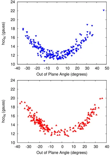
In order to show how the variability in the improper dihedral affects calculated hccNvalues, two different set of calculations were
performed. First, all solvent molecules in all snapshots were removed and hccNwere calculated on the resulting structures. Second, all
sol-vent molecules were indeed included and treated at the FQ level, with the sole inclusion of electrostatic effects (c parametrization). In
Figs. 4and5, the resulting hccNvalues are reported as a function of
the out-of-plane CαNOCαangle.
As expected, the same picture as already reported for the isolated radicals emerges.
FIG. 4. PBE0/N07D calculated hccN (gauss) on the solute-only structures
extracted from MD runs as a function of the out of plane CαNOCαangle. (Top:
PROXYL; bottom: TEMPO).
FIG. 5. PBE0/N07D QM/FQ calculated hccN (gauss) on the entire snapshots
extracted from MD runs as a function of the out of plane CαNOCαangle. (Top:
PROXYL; bottom: TEMPO).
Due to the large variability of hccNvalues as a function of the
out of plane angle, the convergence of average values needs to be carefully checked. InFig. 6, QM/FQ hccNaverage values as a
func-tion of the number of snapshots are depicted for the two radicals. Clearly, hccNis well converged by using 200 snapshots.
Let us now compare our computed data with their experi-mental counterparts.Table VIcollects hccNvalues computed with
different approaches. QM indicates calculations performed on the solute-only structures extracted from MD (see above). QM/FQ data were obtained by using the purely electrostatic polarizable FQ with the c parametrization (the results obtained by exploit-ing the a, b parametrizations are reported in Table S4 in the
supplementary material). The contribution to hccN due to
repul-sion interactions is denoted as ∆rep, whereas the contribution to
hccN of both repulsion and dispersion interactions is denoted
as ∆dis-rep.
We first notice that, due to the different structural sampling given by the MD, the QM data inTable VIdiffer from what was reported for the isolated radicals (seeTable II). The dynamical sam-pling increases PROXYL and TEMPO hccN values by about 2.4
FIG. 6. QM/FQ hccN mean value as a function of the number of snapshots
extracted from MD runs. (Top: PROXYL; bottom: TEMPO) All data are reported in gauss.
and 2.2 gauss, respectively. As a result, the difference between hccN
values of the two radicals (1.1 gauss) is in good agreement with experimental data (0.9 G).103,104 When full solvent effects are
included at the purely electrostatic FQ level (2nd column), hccN
values are increased by about 2.3 gauss on average for both
TABLE VI. PBE0/N07D hccNmean values calculated on 200 snapshots extracted
from MD runs. QM indicates the calculation performed on solute-only structures. FQ refers to the purely electrostatic QM/FQ with c parametrization.∆repand∆dis-repare
differences between FQ and hccNdata obtained with our method. Best QM/MM data
are obtained by summing FQ,∆dis-rep, and∆CC/PBE 0(seeTable IV). All values are
reported in gauss.
Best QM/MM
QM FQ ∆rep ∆dis-rep FQ+∆dis-rep+∆CC/PBE0 Expt.
PROXYL 13.5 15.9 −0.4 −0.4 16.4± 0.1 16.4103
TEMPO 14.6 16.8 −0.5 −0.5 17.1± 0.1 17.3104
radicals. This means that attractive interactions increase the com-puted property. As a result, the inclusion of repulsive interaction terms is expected to decrease computed values, and this is indeed confirmed by the values reported in the third column. In particular, for both radicals, hccNdecreases by 0.4 and 0.5 G, respectively, i.e., of
about 17% and 23% of the whole solvent effect. The further inclusion of dispersion terms does not affect the difference with FQ average values.
In order to best compare the results of our approach with experimental findings, DFT values were also corrected to account for some intrinsic deficiency. To this end, the difference between full DFT and full CCSD data obtained for clusters (∆CC/PBE0, see
Table IV) was added to the calculated QM/MM value. The result-ing values are labeled “Best QM/MM” inTable VI. Remarkably, our best computed values are in excellent agreement with experimental data for both radicals, thus confirming the accuracy and reliability of our approach.
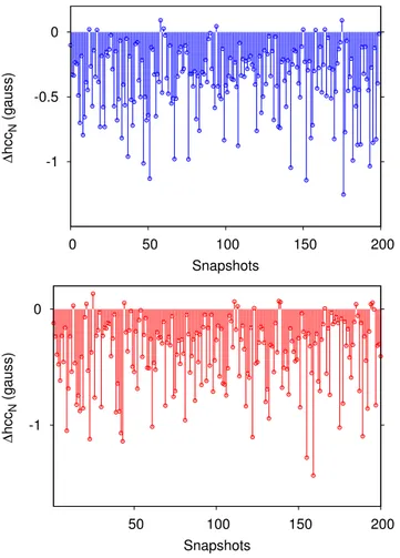
To get further insight into solvent effects on hccNvalues,
dif-ferences between FQ and QM values are reported as a function of the snapshot inFig. 7. As it can be noticed, for both PROXYL (top)
FIG. 7. Calculated solvent effects (see text) on hccNas a function of the snapshot
extracted from MD runs (Top: PROXYL; bottom: TEMPO). All data are reported in Gauss.
FIG. 8. Difference between FQ and QM/FQ+repulsion solvent effects as a function
of the snapshot extracted from the MD (Top: PROXYL; bottom: TEMPO). All data are reported in Gauss.
and TEMPO (bottom), the electrostatic solvent contribution to hccN
is always positive (only in one case, a small negative contribution is reported for TEMPO). Notice that this is different from what has been reported for electric properties of higher order.84
InFig. 8, the difference between calculated solvent effects on hccN as obtained with the purely electrostatic FQ approach or
with the further inclusion of the repulsion contribution is reported. Remarkably, repulsion contributions increase or decrease the hccN
value depending on the selected snapshot, thus showing that clus-ter approaches do not guarantee an adequate modeling of solvent effects. In fact, although repulsion effects give on average a nega-tive contribution to hccN, by taking a random snapshot (cluster), a
completely different picture could emerge. V. SUMMARY AND CONCLUSIONS
In this paper, we have extended to the calculation of hyper-fine coupling constants, the model proposed in Ref.43to include Pauli repulsion and dispersion effects in QM/MM approaches. The peculiarity of the proposed approach stands in the fact that repul-sion/dispersion contributions are explicitly introduced in the QM
Hamiltonian. Therefore, such terms not only enter the evaluation of energetic properties but also, remarkably, propagate to molecular properties and spectra. The account of such contributions has per-mitted a quantitative analysis of QM/MM interaction energies, and this has also required a novel parametrization of the FQ force field, which has been then tested against the prediction of EPR hccN of
PROXYL and TEMPO in aqueous solutions.
Numerical applications to the two radicals in vacuo, solvated within the so-called cluster approach or as modeled through MD, confirm the well known relevance of solvent effects and a proper account of their dynamical aspects. The further inclusion of dis-persion and especially repulsion solute-solvent interactions gives, remarkably, an almost perfect agreement between calculated and experimental values. Therefore, although electrostatic effects have been invoked as dominating the solvation phenomenon in aqueous solution, we found that non-electrostatic effects are indeed relevant, contributing to 17% and 23% of the entire solvent effects on hccN
for PROXYL and TEMPO, respectively. Remarkably, dispersion interactions seem not to play a crucial role.
To end the discussion, we remark that our model is general enough to be applied to any kind of solvent/environment, pending a reliable parametrization of both electrostatic and non-electrostatic interactions. Also, due to the inclusion of all terms in the molecular Hamiltonian, our approach can be extended to any kind of molec-ular properties and spectroscopies; this will be the topic of future communications.
SUPPLEMENTARY MATERIAL
Seesupplementary materialfor PBE0/N07D and CCSD/EPR-II reduced TEMPO hccN values as a function of the out of plane
CαNOCαangle. PROXYL and TEMPO selected geometrical
param-eters at different levels of theory with the inclusion of Grimme empirical dispersion D3. PROXYL+2w interaction energies calcu-lated at the QM/FQ, SAPT0, and CCSD(T) level. O and H parame-ters for FQ calculations. PROXYL and TEMPO hccNcalculated on
200 snapshots extracted from MD runs.
ACKNOWLEDGMENTS
We are thankful for the computer resources provided by the high performance computer facilities of the SMART Labora-tory (http://smart.sns.it/). C.C. gratefully acknowledges the support of H2020-MSCA-ITN-2017 European Training Network “Com-putational Spectroscopy In Natural sciences and Engineering” (COSINE), Grant No. 765739.
REFERENCES
1
J. Tomasi, B. Mennucci, and R. Cammi, “Quantum mechanical continuum solvation models,”Chem. Rev.105, 2999–3094 (2005).
2H. M. Senn and W. Thiel, “QM/MM methods for biomolecular systems,”Angew.
Chem., Int. Ed.48, 1198–1229 (2009).
3
J. R. Cheeseman, M. S. Shaik, P. L. Popelier, and E. W. Blanch, “Calculation of Raman optical activity spectra of methyl-β-d-glucose incorporating a full molecu-lar dynamics simulation of hydration effects,”J. Am. Chem. Soc.133, 4991–4997 (2011).
4B. Mennucci, “Modeling environment effects on spectroscopies through
5
K. H. Hopmann, K. Ruud, M. Pecul, A. Kudelski, M. Draˇcínský, and P. Bour, “Explicit versus implicit solvent modeling of Raman optical activity spectra,” J. Phys. Chem. B115, 4128–4137 (2011).
6
C. Cappelli, F. Lipparini, J. Bloino, and V. Barone, “Towards an accurate descrip-tion of anharmonic infrared spectra in soludescrip-tion within the polarizable continuum model: Reaction field, cavity field and nonequilibrium effects,”J. Chem. Phys.135, 104505 (2011).
7
F. Egidi, T. Giovannini, M. Piccardo, J. Bloino, C. Cappelli, and V. Barone, “Stereoelectronic, vibrational, and environmental contributions to polarizabili-ties of large molecular systems: A feasible anharmonic protocol,”J. Chem. Theory Comput.10, 2456–2464 (2014).
8
C. Cappelli, “Integrated QM/polarizable MM/continuum approaches to model chiroptical properties of strongly interacting solute-solvent systems,”Int. J. Quan-tum Chem.116, 1532–1542 (2016).
9
E. Boulanger and J. N. Harvey, “QM/MM methods for free energies and photo-chemistry,”Curr. Opin. Struct. Biol.49, 72–76 (2018).
10
P. Lahiri, K. B. Wiberg, P. H. Vaccaro, M. Caricato, and T. D. Crawford, “Large solvation effect in the optical rotatory dispersion of norbornenone,” Angew. Chem.126, 1410–1413 (2014).
11
D. Loco, S. Jurinovich, L. Cupellini, M. F. Menger, and B. Mennucci, “The modeling of the absorption lineshape for embedded molecules through a polarizable QM/MM approach,” Photochem. Photobiol. Sci. 17, 552–560 (2018).
12
A. Warshel and M. Levitt, “Theoretical studies of enzymic reactions: Dielec-tric, electrostatic and steric stabilization of the carbonium ion in the reaction of lysozyme,”J. Mol. Biol.103, 227–249 (1976).
13
M. J. Field, P. A. Bash, and M. Karplus, “A combined quantum mechanical and molecular mechanical potential for molecular dynamics simulations,”J. Comput. Chem.11, 700–733 (1990).
14
J. Gao, “Hybrid quantum and molecular mechanical simulations: An alterna-tive avenue to solvent effects in organic chemistry,”Acc. Chem. Res.29, 298–305 (1996).
15
R. A. Friesner and V. Guallar, “Ab initio quantum chemical and mixed quan-tum mechanics/molecular mechanics (QM/MM) methods for studying enzymatic catalysis,”Annu. Rev. Phys. Chem.56, 389–427 (2005).
16
H. Lin and D. G. Truhlar, “QM/MM: What have we learned, where are we, and where do we go from here?,” Theor. Chem. Acc. 117, 185–199 (2007).
17
A. Monari, J.-L. Rivail, and X. Assfeld, “Theoretical modeling of large molec-ular systems. Advances in the local self consistent field method for mixed quan-tum mechanics/molecular mechanics calculations,”Acc. Chem. Res.46, 596–603 (2012).
18A. Monari, T. Very, J.-L. Rivail, and X. Assfeld, “A QM/MM study on the
spinach plastocyanin: Redox properties and absorption spectra,”Comput. Theor. Chem.990, 119–125 (2012).
19P. N. Day, J. H. Jensen, M. S. Gordon, S. P. Webb, W. J. Stevens, M. Krauss,
D. Garmer, H. Basch, and D. Cohen, “An effective fragment method for modeling solvent effects in quantum mechanical calculations,”J. Chem. Phys.105, 1968– 1986 (1996).
20
V. Kairys and J. H. Jensen, “QM/MM boundaries across covalent bonds: A frozen localized molecular orbital-based approach for the effective fragment potential method,”J. Phys. Chem. A104, 6656–6665 (2000).
21
Y. Mao, O. Demerdash, M. Head-Gordon, and T. Head-Gordon, “Assessing ion–water interactions in the amoeba force field using energy decomposition anal-ysis of electronic structure calculations,”J. Chem. Theory Comput.12, 5422–5437 (2016).
22D. Loco, É. Polack, S. Caprasecca, L. Lagardere, F. Lipparini, J.-P. Piquemal, and
B. Mennucci, “A QM/MM approach using the amoeba polarizable embedding: From ground state energies to electronic excitations,”J. Chem. Theory Comput. 12, 3654–3661 (2016).
23
D. Loco and L. Cupellini, “Modeling the absorption lineshape of embedded sys-tems from molecular dynamics: A tutorial review,”Int. J. Quantum Chem.119, e25726 (2019).
24
B. T. Thole, “Molecular polarizabilities calculated with a modified dipole inter-action,”Chem. Phys.59, 341–350 (1981).
25
A. H. Steindal, K. Ruud, L. Frediani, K. Aidas, and J. Kongsted, “Excitation ener-gies in solution: The fully polarizable QM/MM/PCM method,”J. Phys. Chem. B 115, 3027–3037 (2011).
26
S. Jurinovich, C. Curutchet, and B. Mennucci, “The Fenna–Matthews– Olson protein revisited: A fully polarizable (TD) DFT/MM description,” ChemPhysChem15, 3194–3204 (2014).
27
E. Boulanger and W. Thiel, “Solvent boundary potentials for hybrid QM/MM computations using classical drude oscillators: A fully polarizable model,” J. Chem. Theory Comput.8, 4527–4538 (2012).
28
S. W. Rick, S. J. Stuart, and B. J. Berne, “Dynamical fluctuating charge force fields: Application to liquid water,” J. Chem. Phys. 101, 6141–6156 (1994).
29
S. W. Rick and B. J. Berne, “Dynamical fluctuating charge force fields: The aqueous solvation of amides,”J. Am. Chem. Soc.118, 672–679 (1996).
30
T. Giovannini, M. Olszòwka, F. Egidi, J. R. Cheeseman, G. Scalmani, and C. Cappelli, “Polarizable embedding approach for the analytical calculation of Raman and Raman optical activity spectra of solvated systems,”J. Chem. Theory Comput.13, 4421–4435 (2017).
31
F. Lipparini, F. Egidi, C. Cappelli, and V. Barone, “The optical rotation of methyloxirane in aqueous solution: A never ending story?,”J. Chem. Theory Comput.9, 1880–1884 (2013).
32
D. Loco, F. Buda, J. Lugtenburg, and B. Mennucci, “The dynamic origin of color tuning in proteins revealed by a carotenoid pigment,”J. Phys. Chem. Lett.9, 2404– 2410 (2018).
33
J. E. Lennard-Jones, “Cohesion,”Proc. Phys. Soc.43, 461 (1931).
34
E. Boulanger, L. Huang, C. Rupakheti, A. D. MacKerell, Jr., and B. Roux, “Opti-mized Lennard-Jones parameters for druglike small molecules,”J. Chem. Theory Comput.14, 3121–3131 (2018).
35
M. S. Gordon, Q. A. Smith, P. Xu, and L. V. Slipchenko, “Accurate first prin-ciples model potentials for intermolecular interactions,”Annu. Rev. Phys. Chem. 64, 553–578 (2013).
36
H. Gokcan, E. G. Kratz, T. A. Darden, J.-P. Piquemal, and G. A. Cisneros, “QM/MM simulations with the Gaussian electrostatic model, a density-based polarizable potential,”J. Phys. Chem. Lett.9, 3062–3067 (2018).
37
M. S. Gordon, L. Slipchenko, H. Li, and J. H. Jensen, “The effective fragment potential: A general method for predicting intermolecular interactions,”Annu. Rep. Comput. Chem.3, 177–193 (2007).
38
M. S. Gordon, M. A. Freitag, P. Bandyopadhyay, J. H. Jensen, V. Kairys, and W. J. Stevens, “The effective fragment potential method: A QM-based MM approach to modeling environmental effects in chemistry,”J. Phys. Chem. A105, 293–307 (2001).
39I. Adamovic and M. S. Gordon, “Dynamic polarizability, dispersion coefficient
C6and dispersion energy in the effective fragment potential method,”Mol. Phys.
103, 379–387 (2005).
40L. V. Slipchenko, “Effective fragment potential method,” in Many-Body Effects
and Electrostatics in Biomolecules (Pan Stanford, 2016), pp. 147–187.
41
J. M. H. Olsen, C. Steinmann, K. Ruud, and J. Kongsted, “Polarizable density embedding: A new QM/QM/MM-based computational strategy,”J. Phys. Chem. A119, 5344–5355 (2015).
42
P. Reinholdt, J. Kongsted, and J. M. H. Olsen, “Polarizable density embedding: A solution to the electron spill-out problem in multiscale modeling,”J. Phys. Chem. Lett.8, 5949–5958 (2017).
43
T. Giovannini, P. Lafiosca, and C. Cappelli, “A general route to include Pauli repulsion and quantum dispersion effects in QM/MM approaches,”J. Chem. Theory Comput.13, 4854–4870 (2017).
44
A. Tkatchenko and M. Scheffler, “Accurate molecular van der Waals interac-tions from ground-state electron density and free-atom reference data,”Phys. Rev. Lett.102, 073005 (2009).
45
A. Tkatchenko, L. Romaner, O. T. Hofmann, E. Zojer, C. Ambrosch-Draxl, and M. Scheffler, “Van der Waals interactions between organic adsorbates and at organic/inorganic interfaces,” MRS Bull. 35, 435–442 (2010).
46A. Tkatchenko, R. A. DiStasio, Jr., R. Car, and M. Scheffler, “Accurate and
effi-cient method for many-body van der Waals interactions,”Phys. Rev. Lett.108, 236402 (2012).
47
J. Hermann, R. A. DiStasio, and A. Tkatchenko, “First-principles models for van der Waals interactions in molecules and materials: Concepts, theory, and applications,”Chem. Rev.117, 4714–4758 (2017).
48C. Curutchet, L. Cupellini, J. Kongsted, S. Corni, L. Frediani, A. H.
Stein-dal, C. A. Guido, G. Scalmani, and B. Mennucci, “Density-dependent formula-tion of dispersion–repulsion interacformula-tions in hybrid multiscale quantum/molecular mechanics (QM/MM) models,”J. Chem. Theory Comput.14, 1671–1681 (2018).
49
G. A. Cisneros, J.-P. Piquemal, and T. A. Darden, “Intermolecular electrostatic energies using density fitting,”J. Chem. Phys.123, 044109 (2005).
50
J.-P. Piquemal, G. A. Cisneros, P. Reinhardt, N. Gresh, and T. A. Darden, “Towards a force field based on density fitting,”J. Chem. Phys.124, 104101 (2006).
51
G. A. Cisneros, J.-P. Piquemal, and T. A. Darden, “Generalization of the Gaus-sian electrostatic model: Extension to arbitrary angular momentum, distributed multipoles, and speedup with reciprocal space methods,”J. Chem. Phys.125, 184101 (2006).
52
M. Pavone, P. Cimino, F. De Angelis, and V. Barone, “Interplay of stereoelec-tronic and environmental effects in tuning the structural and magnetic properties of a prototypical spin probe: Further insights from a first principle dynamical approach,”J. Am. Chem. Soc.128, 4338–4347 (2006).
53
V. Barone, “Electronic, vibrational and environmental effects on the hyperfine coupling constants of nitroxide radicals. H2NO as a case study,”Chem. Phys. Lett.
262, 201–206 (1996).
54
R. Improta and V. Barone, “Interplay of electronic, environmental, and vibra-tional effects in determining the hyperfine coupling constants of organic free radicals,”Chem. Rev.104, 1231–1254 (2004).
55
M. Pavone, P. Cimino, O. Crescenzi, A. Sillanpaeae, and V. Barone, “Interplay of intrinsic, environmental, and dynamic effects in tuning the EPR parameters of nitroxides: Further insights from an integrated computational approach,”J. Phys. Chem. B111, 8928–8939 (2007).
56
V. Barone, P. Cimino, O. Crescenzi, and M. Pavone, “Ab initio computation of spectroscopic parameters as a tool for the structural elucidation of organic systems,”J. Mol. Struct.: THEOCHEM811, 323–335 (2007).
57
M. Pavone, A. Sillanpää, P. Cimino, O. Crescenzi, and V. Barone, “Evidence of variable H-bond network for nitroxide radicals in protic solvents,”J. Phys. Chem. B110, 16189–16192 (2006).
58
V. Barone, M. Brustolon, P. Cimino, A. Polimeno, M. Zerbetto, and A. Zoleo, “Development and validation of an integrated computational approach for the modeling of cw-ESR spectra of free radicals in solution: p-(methylthio) phenyl nitronylnitroxide in toluene as a case study,”J. Am. Chem. Soc.128, 15865–15873 (2006).
59
E. Stendardo, A. Pedone, P. Cimino, M. C. Menziani, O. Crescenzi, and V. Barone, “Extension of the amber force-field for the study of large nitroxides in condensed phases: An ab initio parameterization,”Phys. Chem. Chem. Phys. 12, 11697–11709 (2010).
60
V. Barone, P. Cimino, and A. Pedone, “An integrated computational protocol for the accurate prediction of EPR and PNMR parameters of aminoxyl radicals in solution,”Magn. Reson. Chem.48, S11–S22 (2010).
61
J. C. Schöneboom, F. Neese, and W. Thiel, “Toward identification of the com-pound I reactive intermediate in cytochrome P450 chemistry: A QM/MM study of its EPR and Mössbauer parameters,”J. Am. Chem. Soc.127, 5840–5853 (2005).
62
S. Sinnecker and F. Neese, “QM/MM calculations with DFT for taking into account protein effects on the EPR and optical spectra of metalloproteins. Plas-tocyanin as a case study,”J. Comput. Chem.27, 1463–1475 (2006).
63
S. Moon, S. Patchkovskii, and D. R. Salahub, “QM/MM calculations of EPR hyperfine coupling constants in blue copper proteins,” J. Mol. Struct.: THEOCHEM632, 287–295 (2003).
64
H. M. Senn and W. Thiel, “QM/MM studies of enzymes,”Curr. Opin. Chem. Biol.11, 182–187 (2007).
65
V. Barone, A. Bencini, M. Cossi, A. D. Matteo, M. Mattesini, and F. Totti, “Assessment of a combined QM/MM approach for the study of large nitroxide systems in vacuo and in condensed phases,”J. Am. Chem. Soc.120, 7069–7078 (1998).
66
L. J. Berliner, Spin Labeling: Theory and Applications (Academic, New York, 1976).
67
N. Kocherginsky and H. M. Swartz, Nitroxide Spin Labels: Reactions in Biology and Chemistry (CRC Press, New York, 1995).
68
A. H. Buchaklian and C. S. Klug, “Characterization of the walker a motif of MsbA using site-directed spin labeling electron paramagnetic resonance spec-troscopy,”Biochemistry44, 5503–5509 (2005).
69
M. Engström, O. Vahtras, and H.Ågren, “MCSCF and DFT calculations of EPR parameters of sulfur centered radicals,”Chem. Phys. Lett.328, 483–491 (2000).
70
Z. Rinkevicius, B. Frecus, N. A. Murugan, O. Vahtras, J. Kongsted, and H.Ågren, “Encapsulation influence on EPR parameters of spin-labels: 2, 2, 6, 6-tetramethyl-4-methoxypiperidine-1-oxyl in cucurbit[8]uril,”J. Chem. Theory Comput.8, 257–263 (2011).
71
K. J. de Almeida, Z. Rinkevicius, H. W. Hugosson, A. C. Ferreira, and H.Ågren, “Modeling of EPR parameters of copper (II) aqua complexes,”Chem. Phys.332, 176–187 (2007).
72
C. Di Valentin, G. Pacchioni, A. Selloni, S. Livraghi, and E. Giamello, “Charac-terization of paramagnetic species in N-doped TiO2powders by EPR spectroscopy
and DFT calculations,”J. Phys. Chem. B109, 11414–11419 (2005).
73
M. Anpo, Y. Shioya, H. Yamashita, E. Giamello, C. Morterra, M. Che, H. H. Patterson, S. Webber, and S. Ouellette, “Preparation and characterization of the Cu+/zsm-5 catalyst and its reaction with NO under UV irradiation at 275 K. In situ photoluminescence, EPR, and FT-IR investigations,”J. Phys. Chem.98, 5744– 5750 (1994).
74J.-L. Clément, N. Ferré, D. Siri, H. Karoui, A. Rockenbauer, and P. Tordo,
“Assignment of the EPR spectrum of 5, 5-dimethyl-1-pyrroline N-oxide (DMPO) superoxide spin adduct,”J. Org. Chem.70, 1198–1203 (2005).
75E. Giner, L. Tenti, C. Angeli, and N. Ferré, “Computation of the isotropic
hyper-fine coupling constant: Efficiency and insights from a new approach based on wave function theory,”J. Chem. Theory Comput.13, 475–487 (2017).
76C. Amovilli and R. McWeeny, “A matrix partitioning approach to the
calcu-lation of intermolecular potentials. General theory and some examples,”Chem. Phys.140, 343–361 (1990).
77R. McWeeny, Methods of Molecular Quantum Mechanics (Academic Press,
London, 1992).
78
F. Lipparini and V. Barone, “Polarizable force fields and polarizable continuum model: A fluctuating charges/PCM approach. 1. Theory and implementation,” J. Chem. Theory Comput.7, 3711–3724 (2011).
79
F. Lipparini, C. Cappelli, G. Scalmani, N. De Mitri, and V. Barone, “Analyti-cal first and second derivatives for a fully polarizable QM/classi“Analyti-cal Hamiltonian,” J. Chem. Theory Comput.8, 4270–4278 (2012).
80
T. Giovannini, M. Olszowka, and C. Cappelli, “Effective fully polarizable QM/MM approach to model vibrational circular dichroism spectra of systems in aqueous solution,”J. Chem. Theory Comput.12, 5483–5492 (2016).
81
T. Giovannini, G. Del Frate, P. Lafiosca, and C. Cappelli, “Effective compu-tational route towards vibrational optical activity spectra of chiral molecules in aqueous solution,”Phys. Chem. Chem. Phys.20, 9181–9197 (2018).
82
T. Giovannini, M. Macchiagodena, M. Ambrosetti, A. Puglisi, P. Lafiosca, G. Lo Gerfo, F. Egidi, and C. Cappelli, “Simulating vertical excitation energies of solvated dyes: From continuum to polarizable discrete modeling,”Int. J. Quantum Chem. 119, e25684 (2019).
83F. Lipparini, C. Cappelli, and V. Barone, “Linear response theory and electronic
transition energies for a fully polarizable QM/classical Hamiltonian,”J. Chem. Theory Comput.8, 4153–4165 (2012).
84T. Giovannini, M. Ambrosetti, and C. Cappelli, “A polarizable embedding
approach to second harmonic generation (SHG) of molecular systems in aqueous solutions,”Theor. Chem. Acc.137, 74 (2018).
85C. Amovilli and B. Mennucci, “Self-consistent-field calculation of Pauli
repul-sion and disperrepul-sion contributions to the solvation free energy in the polarizable continuum model,”J. Phys. Chem. B101, 1051–1057 (1997).
86F. L. Hirshfeld, “Bonded-atom fragments for describing molecular charge
densities,”Theor. Chem. Acc.44, 129–138 (1977).
87
I. Harczuk, B. Nagy, F. Jensen, O. Vahtras, and H.Ågren, “Local decomposi-tion of imaginary polarizabilities and dispersion coefficients,”Phys. Chem. Chem. Phys.19, 20241–20250 (2017).
88
S. Grimme, “Density functional theory with London dispersion corrections,” Wiley Interdiscip. Rev.: Comput. Mol. Sci1, 211–228 (2011).
89
S. Grimme, J. Antony, S. Ehrlich, and H. Krieg, “A consistent and accurate ab initio parametrization of density functional dispersion correction (DFT-D) for the 94 elements H-Pu,”J. Chem. Phys.132, 154104 (2010).
90
O. L. Malkina, J. Vaara, B. Schimmelpfennig, M. Munzarová, V. G. Malkin, and M. Kaupp, “Density functional calculations of electronic g-tensors using spin-orbit pseudopotentials and mean-field all-electron spin-spin-orbit operators,”J. Am. Chem. Soc.122, 9206–9218 (2000).
91
M. Kaupp, C. Remenyi, J. Vaara, O. L. Malkina, and V. G. Malkin, “Density functional calculations of electronic g-tensors for semiquinone radical anions. The role of hydrogen bonding and substituent effects,”J. Am. Chem. Soc.124, 2709– 2722 (2002).
92
V. Barone and P. Cimino, “Accurate and feasible computations of structural and magnetic properties of large free radicals: The PBE0/N07D model,”Chem. Phys. Lett.454, 139–143 (2008).
93
V. Barone, P. Cimino, and E. Stendardo, “Development and validation of the B3LYP/N07D computational model for structural parameter and mag-netic tensors of large free radicals,” J. Chem. Theory Comput. 4, 751–764 (2008).
94
V. Barone, “Structure, magnetic properties and reactivities of open-shell species from density functional and self-consistent hybrid methods,” in Recent Advances in Density Functional Methods: Part I (World Scientific, 1995), pp. 287–334.
95
R. M. Parrish, L. A. Burns, D. G. A. Smith, A. C. Simmonett, A. E. DePrince, E. G. Hohenstein, U. Bozkaya, A. Y. Sokolov, R. Di Remigio, R. M. Richard, J. F. Gonthier, A. M. James, H. R. McAlexander, A. Kumar, M. Saitow, X. Wang, B. P. Pritchard, P. Verma, H. F. Schaefer, K. Patkowski, R. A. King, E. F. Valeev, F. A. Evangelista, J. M. Turney, T. D. Crawford, and C. D. Sherrill, “Psi4 1.1: An open-source electronic structure program emphasizing automation, advanced libraries, and interoperability,”J. Chem. Theory Comput.13, 3185–3197 (2017).
96
P. Mark and L. Nilsson, “Structure and dynamics of the TIP3P, SPC, and SPC/E water models at 298 K,”J. Phys. Chem. A105, 9954–9960 (2001).
97I. Carnimeo, C. Cappelli, and V. Barone, “Analytical gradients for MP2,
dou-ble hybrid functionals, and TD-DFT with polarizadou-ble embedding described by fluctuating charges,”J. Comput. Chem.36, 2271–2290 (2015).
98V. Hornak, R. Abel, A. Okur, B. Strockbine, A. Roitberg, and C. Simmerling,
“Comparison of multiple amber force fields and development of improved protein backbone parameters,”Proteins65, 712–725 (2006).
99D. A. Case, T. E. Cheatham, T. Darden, H. Gohlke, R. Luo, K. M. Merz,
A. Onufriev, C. Simmerling, B. Wang, and R. J. Woods, “The amber biomolecular simulation programs,”J. Comput. Chem.26, 1668–1688 (2005).
100
J.-P. Ryckaert, G. Ciccotti, and H. J. Berendsen, “Numerical integration of the Cartesian equations of motion of a system with constraints: Molecular dynamics of n-alkanes,”J. Comput. Phys.23, 327–341 (1977).
101T. Darden, D. York, and L. Pedersen, “Particle mesh Ewald: An N log(N)
method for Ewald sums in large systems,”J. Chem. Phys.98, 10089–10092 (1993).
102
M. J. Frisch, G. W. Trucks, H. B. Schlegel, G. E. Scuseria, M. A. Robb, J. R. Cheeseman, G. Scalmani, V. Barone, G. A. Petersson, H. Nakatsuji, X. Li, M. Cari-cato, A. V. Marenich, J. Bloino, B. G. Janesko, R. Gomperts, B. Mennucci, H. P. Hratchian, J. V. Ortiz, A. F. Izmaylov, J. L. Sonnenberg, D. Williams-Young, F. Ding, F. Lipparini, F. Egidi, J. Goings, B. Peng, A. Petrone, T. Henderson, D. Ranasinghe, V. G. Zakrzewski, J. Gao, N. Rega, G. Zheng, W. Liang, M. Hada, M. Ehara, K. Toyota, R. Fukuda, J. Hasegawa, M. Ishida, T. Nakajima, Y. Honda, O. Kitao, H. Nakai, T. Vreven, K. Throssell, J. A. Montgomery, Jr., J. E. Peralta, F. Ogliaro, M. J. Bearpark, J. J. Heyd, E. N. Brothers, K. N. Kudin, V. N. Staroverov, T. A. Keith, R. Kobayashi, J. Normand, K. Raghavachari, A. P. Rendell, J. C. Burant, S. S. Iyengar, J. Tomasi, M. Cossi, J. M. Millam, M. Klene, C. Adamo, R. Cammi, J. W. Ochterski, R. L. Martin, K. Morokuma, O. Farkas, J. B. Fores-man, and D. J. Fox, Gaussian 16, Revision A.03, Gaussian Inc., Wallingford, CT, 2016.
103
J. F. Keana, T. D. Lee, and E. M. Bernard, “Side-chain substituted 2, 2, 5, 5-tetramethylpyrrolidine-N-oxyl (proxyl) nitroxides. A new series of lipid spin labels showing improved properties for the study of biological membranes,”J. Am. Chem. Soc.98, 3052–3053 (1976).
104A. Rockenbauer, L. Korecz, and K. Hideg, “Ring pseudorotation in pyrrolidine
N-oxyl radicals: An analysis of 13C-hyperfine structure of EPR spectra,”J. Chem. Soc., Perkin Trans. 20(11), 2149–2156 (1993).
105C. Puzzarini and V. Barone, “Diving for accurate structures in the ocean of
molecular systems with the help of spectroscopy and quantum chemistry,”Acc. Chem. Res.51, 548–556 (2018).
106K. Szalewicz, “Symmetry-adapted perturbation theory of intermolecular
forces,”Wiley Interdiscip. Rev.: Comput. Mol. Sci.2, 254–272 (2012).
107
E. G. Hohenstein and C. D. Sherrill, “Wavefunction methods for non-covalent interactions,”Wiley Interdiscip. Rev.: Comput. Mol. Sci2, 304–326 (2012).
108
T. M. Parker, L. A. Burns, R. M. Parrish, A. G. Ryno, and C. D. Sherrill, “Levels of symmetry adapted perturbation theory (SAPT). I. Efficiency and performance for interaction energies,”J. Chem. Phys.140, 094106 (2014).
109
S. F. Boys and F. d. Bernardi, “The calculation of small molecular interac-tions by the differences of separate total energies. Some procedures with reduced errors,”Mol. Phys.19, 553–566 (1970).