Universit`
a degli Studi di Pisa
Technische Universiteit Delft
Facolt`
a di Ingegneria
Corso di Laurea Specialistica in
Ingegneria dei Veicoli Terrestri
Tesi di Laurea
“Feasibility Study of Yaw Control by
active 4-Wheel Drive”
Marco Ghelardoni
Relatori:
Prof. Ing. Massimo Guiggiani (Universit`a degli Studi di Pisa)
Prof. Ing. Giuseppe Forasassi (Universit`a degli Studi di Pisa)
Ir. Edwin J. H. de Vries (Delft University of Technology)
28 Ottobre 2004 Anno Accademico 2003/2004
Abstract
In this research we analyze the feasibility of an Active Yaw Control whose working principle is based on the engine torque distribution between the front and the rear axle of the vehicle. In addition we compare our system with a traditional ESP (Electronic Stability Program) and we study the possibility to make these systems cooperate. We simulated the car motion in several different conditions, for example in case of high cornering speed or during an avoidance manoeuvre. The vehicle behavior is evaluated in terms of stability, handling, performance and comfort. The models of the vehicle and of the other devices are built using the software “Simulink”. It was concluded that providing a vehicle that is normally rear-wheel drive with our system we can create contra-cornering yaw moments. To produce a pro-cornering yaw moment is possible when our Active Yaw Control is applied on a front-wheel drive car. Therefore the redistribution of torque system is not able to prevent both oversteer and understeer on the same vehicle. On the contrary the ESP can correct both of these undesired motions. Moreover the ESP proved to be more powerful than our method but even more uncomfortable and, whereas it acts on the brake system, it makes the car performance worse. In the end we established that the ESP and the redistribution of torque strategy can work together without interfering negatively, improving the effectiveness of the Active Yaw Control interventions.
Contents
0.1 List of Symbols . . . iii
1 Introduction 1 1.1 Electronic Control Systems History . . . 2
2 Vehicle Model 5 2.1 Vehicle Model . . . 5 2.1.1 Vehicle equations . . . 6 2.1.2 Vertical Load . . . 7 2.1.3 On Demand Drive . . . 8 2.2 Tyre Model . . . 12 2.2.1 Reference Frame . . . 12 2.2.2 Slip Quantities . . . 13 2.2.3 Semi-Empirical Model . . . 14 3 Simulink Model 17 3.1 Simulink Model . . . 17 3.1.1 Vehicle Subsystem . . . 17 3.1.2 Tyre Subsystem . . . 19 3.1.3 Engine Model . . . 23
3.1.4 Haldex Coupling Model . . . 24
4 Active Yaw Control 26 4.1 ESP . . . 26
4.1.1 ESP Working Principles . . . 26
4.1.2 ESP Simulink Model . . . 27
4.1.3 “Reference Yaw Rate” Value . . . 27
4.1.4 “Lateral Acceleration” Difference . . . 32
4.1.5 ESP Strategy . . . 33
5 Redistribution of Torque 37 5.1 Drive Torque Control . . . 39
6 Rear-Wheel Drive Car simulations 41
6.1 High Speed A . . . 41
6.2 High Speed B . . . 55
6.3 External Disturbance . . . 57
6.4 Avoidance Manoeuvre . . . 60
7 Front-Wheel Drive Car Simulations 63 7.1 High Speed . . . 63
7.2 External Disturbance . . . 65
7.3 Avoidance Manoeuvre A . . . 68
7.4 Avoidance Manoeuvre B . . . 69
8 Conclusions 72 A Rear-Wheel Drive Car Simulations II 74 A.1 External Disturbance (Understeer, 195/65-R15) . . . 74
A.2 External Disturbance (195/65-R15) . . . 77
A.3 High Speed (205/55-R15) . . . 81
A.4 External Disturbance (205/55-R15) . . . 86
A.5 Avoidance Manoeuvre (205/55-R15) . . . 91
B Front-Wheel Drive Car Simulations II 95 B.1 External Disturbance (Oversteer, 195/65-R15) . . . 95
B.2 High Speed (205/55-R15) . . . 99
B.3 Avoidance Manoeuvre (205/55-R15) . . . 102
C Simulink Model Parameters 107 C.1 M-File . . . 108
C.2 Controllers . . . 110
C.2.1 Rear-Wheel Drive Vehicle . . . 110
0.1
List of Symbols
Symbol Name Unit
————- ——————————————————————————– ———–
a Distance center of gravity - front axle m
a1 Magic Formula coefficient, Dy N−1
a2 Magic Formula coefficient, Dy
-a3 Magic Formula coefficient, BCDy N
a4 Magic Formula coefficient, BCDy N
a6 Magic Formula coefficient, Ey N−1
a7 Magic Formula coefficient, Ey
-B Stiffness factor, Magic Formula
-b Distance center of gravity - rear axle m
b1 Magic Formula coefficient, Dx N−1
b2 Magic Formula coefficient, Dx
-b3 Magic Formula coefficient, BCDx N−1
b4 Magic Formula coefficient, BCDx
-b5 Magic Formula coefficient, BCDx N−1
b6 Magic Formula coefficient, Ex N−2
b7 Magic Formula coefficient, Ex N−1
b8 Magic Formula coefficient, Ex
-C Shape factor, Magic Formula
-Ci Cornering stiffness, front and rear axle N/rad
Cx Drag coefficient, car
-D Peak factor, Magic Formula N
d Roll center height, front and rear axle m
d1 Roll axis height under the center of gravity m
E Curvature Factor, Magic Formula
-e Distance external lateral force m
FL Lateral external force N
Fx(nm) Longitudinal force, tyre N
Fx0(nm) Longitudinal force in pure longitudinal slip conditions, tyre N
Fy(nm) Side force, tyre N
Fy0(nm) Side force in pure side slip conditions, tyre N
Fz Vertical load N
Hnm Distance between the wheel slip axis and the street m
h Center of gravity height m
J Moment of inertia around z axis, car kg m2
Jω(n,m) Moment of inertia around spin axis, wheel kg m2
k Longitudinal slip
Symbol Name Unit
————- ——————————————————————————— ———–
kφi Rolling stiffness, front and rear axle N/rad
L Relaxation length m
l Wheelbase m
Mcl Drive torque provided by the central coupling Nm
Men Drive torque provided by the engine Nm
Mnm Drive torque applied to the wheel Nm
Mb,nm Brake torque Nm
m Mass, car kg
N Total yaw moment Nm
R Corner radius m
Rest Estimated corner radius m
Rref Reference corner radius m
r Yaw rate, car rad/s
rref Reference yaw rate rad/s
re Rolling radius in free rolling conditions, tyre m
Tf0 Maximum drive torque transferrable Nm
by means of the “Haldex” coupling
t Track m
u Longitudinal speed, car m/s
u Estimated longitudinal speed m/s
VG Center of gravity speed, car m/s
Vx X-direction speed, tyre m/s
v Lateral speed, car m/s
X Total longitudinal force N
Y Total lateral force N
δ Steer angle rad
µx Longitudinal friction coefficient
-µy Side friction coefficient
-αnm Slip angle, tyre rad
β Slip angle, car rad
σ Total theoretical slip
-σx Theoretical longitudinal slip
-σy Theoretical side slip
-τd Transmission ratio, differential
-φ Roll angle rad
ω Rotational speed, wheel rad/s
ω0 Rotational speed in free rolling conditions, wheel rad/s
Chapter 1
Introduction
Nowadays many cars are provided with electronic systems able to prevent dangerous
vehi-cle motions (oversteer or understeer1) in order to improve vehicle handling and stability.
Several reasons can cause an unforeseen vehicle behavior, for example the excessive cor-nering speed or the unexpected change of the road grip. These systems, called Active Yaw Control [8], can introduce a yaw moment using various actuator concepts. The stability system intervention in fact can be directed towards the brake system (ESP), the steer angle (of both front and rear wheels), the active suspensions (dynamic drive). In any case the most common among these systems is surely the “ESP” (Electronic Stability Program). This system is very safe, but its action can be uncomfortable or even disappointing for some particular applications, as for example when installed in sport cars. Since the distribution of the engine torque between the front and the rear axle affects the vehicle handling we analyzed the opportunity to exploit this phenomenon in order to increase vehicle safety. In this research, made in cooperation with the “Delft University of Technology” (The Netherlands) within the “Socrates” project 2003-2004, we studied both the possibility to substitute a traditional ESP with a new generation of stability systems, based on the re-distribution of drive torque, and the possibility to use these systems together.
We analyzed the effects caused by the action of these systems in terms of safety, perfor-mance and comfort.
In the second chapter of this report the theoretical vehicle model we used is illustrated and in the third chapter the principal aspects of the “Simulink” model we built to simulate the car behavior are described. The fourth and the fifth chapters deal with the ESP and
1
With the terms oversteer and understeer we will not refer to rigorous definitions but we want to indicate a car behavior which makes the car drive along respectively a wider or a smaller curve radius than the corner radius the driver is used to expect.
the “Redistribution of Torque System” respectively. In the sixth and seventh chapter we illustrate the results obtained by means of the simulations, and in the end we present our conclusions in the eighth chapter.
1.1
Electronic Control Systems History
Until the second half of the 70’s the car motion was controlled just by the driver’s skills. No active-safety devices had been designed before and only the quality of the mechanical project influenced the vehicle safety and stability.
In fact the main contribution to the development of the systems which currently are very common as the “ABS” (Anti Brake-locking System), the “ASR” (Acceleration Skid Control) or the “ESP” (fig. 1.1) was given by the incredibly fast improvement of the electronic components.
Figure 1.1: Main safe systems installed on the vehicles
The first application of this spreading technology was the “ABS”, installed at first on the Mercedes S Class in the 1978 and subsequently on the BMW Series 7. In 25 years this system has been improved very much and it has become a standard equipment for almost the 70% of the production cars.
Year Weight [kg] Number of components Memory [kByte]
1978 6.7 140 2
1995 4.9 40 8
1999 2.6 25 24
2003 1.6 16 128
The second step was the “ASR”, which is a system that does not allow the tyres to slip in case of excessive acceleration. This device, which is interfaced with the “ABS” CPU was thrown on the market in the 1986.
In the end the modern state of art of the electronic control systems is the “ESP”. It was installed at first on a Mercedes in the 1995.
Figure 1.2: Evolution of the electronic systems
By means of this device it is possible to control directly the vehicle motion, the car trajectory, not only the tyre grip. The ESP is spreading very quickly, even faster than the ABS did. In the 2003 it was already installed on almost the 30% of the new vehicles in Europe, however with very different percentages in each country. For example in Germany the 50% of the production vehicles are currently provided with the ESP, but this value decreases at 30% in France, 25% in Spain, 20% in UK and only the 14% in Italy. This last statistical information is very disappointing if we take into account the fact that several studies demonstrate that the ESP can prevent many accidents.
Figure 1.3: Estimated influence of the ESP on the number of accidents
The ESP can be very helpful in order to achieve the target, intended by the UE, to halve the number of victims caused by the car accidents (currently in Europe there are 1.3 millon of accidents each year and the victims are almost 40000).
In the near future the ESP will be interfaced with the active steer system (Bosch is developing this system in cooperation with BMW, which is already providing its luxury vehicles with this device), such a way to make the stability control system faster, safer and more comfortable.
Chapter 2
Vehicle Model
2.1
Vehicle Model
To examine car behavior a vehicle model was built using the software “Simulink”. In this chapter the theoretical aspects are described, but in the next one we focus more specifically on the model actually built.
The model is a four wheeled model, in fact to consider only a simpler and surely more common “Single Track Model” ( [6], [11]) is not possible on account of several reasons
• Some simplifications used to justify the “Single Track Model” are not valid if only
one wheel is braked1, as occurs when the ESP is acting.
• To find a strategy to control the distribution of torque and to model the ESP it is necessary to analyze individual wheel speeds.
• We were interested in studying vehicle behavior in critical conditions (for example a car that is spinning around).
The vehicle is modeled as a rigid body in 2-D; car motions are possible in the horizontal x − y plane, the wheels have no mass but an inertia moment different from zero. The steer axes are considered exactly vertical and passing through the wheel symmetry planes and the wheel spin axes.
The street is schematized like perfectly flat (no slope and roughness). the model is characterized by 7 d.o.f.
More details are shown subsequently.
1
Indeed in the “Single Track Model” the left and the right tyre of an axle must transfer the same longitudinal force
2.1.1
Vehicle equations
Considering the simplifications mentioned above it is possible to build a model based on the subsequent system of equations [6] (see also fig. 2.1):
Figure 2.1: Representation of the principal model quantities
m( ˙u − vr) = X = (Fx11+ Fx12) cos δ − (Fy11+ Fy12) sin δ + (Fx21+ Fx22) −
1 2rCxu
2 (2.1)
m( ˙v + ur) = Y = (Fx11+ Fx12) sin δ + (Fy11+ Fy12) cos δ + (Fy21+ Fy22) + FL (2.2)
J ˙r = N = ((Fx11+ Fx12) sin δ + (Fy11+ Fy12) cos δ)a − (Fy21+ Fy22)b+
−((Fx11− Fx12) cos δ + (Fx21− Fx22) − (Fy11− Fy12) sin δ)t2 + FLe
(2.3)
Jw,nm˙ωnm = Mnm− Fx,nmHnm− Mb,nm, n, m = 1, 2. (2.4)
Although the equations are quite general and not linearized, they present some simpli-fications, for example
• The drag force is applied along the car symmetry axis, without considering lateral actions.
• The external force FL is a pure side force (it does not have drag component).
• The vertical deformations of the tyres are ignored.
• The center of gravity is placed on the car symmetry axis.
2.1.2
Vertical Load
To describe correctly the tyre behavior, knowing the vertical load acting on each wheel, is essential for our problem. In our model only the effect of lateral load transfer is modelled, ignoring modest effects of longitudinal load transfer. We used the following relations, in which we consider the vehicle in a steady state, not to make the problem uselessly compli-cated.
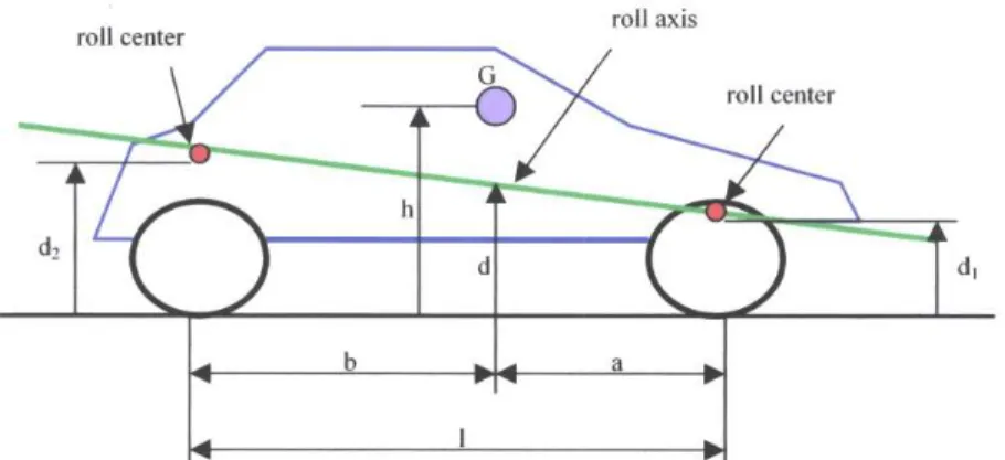
Figure 2.2: Lateral view of the vehicle scheme For the lateral balance of the whole vehicle
Fy1+ Fy2+ FL = Y = mur (2.5)
Fy(1,2) are the global side forces respectively of the front and the rear axle.
For the rotational balance of suspended mass with respect to the roll axis (supposed
horizontal and at a distance d = bd1+ad2
l from the ground)
Figure 2.3: Frontal view of the vehicle scheme
The lateral force (FL), that for example can be considered a representation of lateral
wind, is applied at the same height of the center of gravity. Also this assumption is a simplification.
For rotational balance of each axle (considered with mass equal to zero), with respect to the rolling axis
−∆Fziti+ Fyidi+ kφiφ = 0 (2.7)
Using the previous system of equations, calling Y −FL= ¯Y , we can obtain the following
results ∆Fz1 = (Fy1d1+ kφ1 ¯ Y (h − d) kφ )1 t (2.8) ∆Fz2 = (Fy2d2+ kφ2 ¯ Y (h − d) kφ )1 t (2.9)
Where kφ1,2 are the front and rear axle rolling stiffnesses, kφ is the sum of the two
stiffnesses, d1,2 are the heights of the front and the rear axle roll centers, d is the roll axis
height under the mass center, and in the end h is the mass center height, as shown in fig.2.2 and fig.2.3.
2.1.3
On Demand Drive
Our model represents an on demand drive car. In this kind of vehicles the engine torque is normally directed towards the front or the rear axle but by means of some devices we can split it, such a way to provide torque to all the wheels. It can be really useful in
some situations, for example if the driver is speeding up so hard to make the tyres slip. In fact during a transitory like that we waste uselessly part of the engine power then we do not obtain the maximum possible acceleration and in the same time we can have an excessive wear and tear of the tyres. Sharing the drive torque between the two axles we can avoid these phenomena and improve the vehicle performances. Moreover also the car handling is affected by the drive torque flow. These considerations make us understand that we would like to choose the torque distribution just depending on the configuration which allows the best vehicle performances. Unfortunately this is not possible, at least using conventional apparatuses. Indeed to realize an on demand drive we must equip the vehicle with a central coupling (for example it can be a clutch or a viscous coupling) and they are able just to transfer a part of the whole drive torque. For example, considering a rear-wheel drive vehicle (which torque distribution is 0% − 100%), we can imagine to be allowed to reach a situation in which we have 50% − 50%, but in normal friction conditions we cannot obtain a total inversion of the torque, that is to say 100% − 0%.
We modelled a car provided with an “Haldex” coupling, which is similar to a central clutch, but it can be controlled to regulate the torque flow.
Haldex Coupling
The “Haldex” central coupling is schematically represented in fig.2.4. There is a housing,
connected with the right shaft, which is in turn connected with one of the two differentials installed on the car. This housing has inside the external discs of a wet multi-plate clutch through which torque can be transmitted from the front axle to the rear (or vice versa), a little hydraulic circuit, a valve to control the liquid pressure, a little hydraulic piston pump and a clutch piston that can press the clutch plates each other. The left shaft (linked with the other differential) is connected with the internal clutch plates. At its end, inside the housing, a cam that activates the pump is realized. The pump will only be active when the front and the rear axles rotate at a different speed. The liquid pressure pushes the clutch piston, which engages the clutch. In this way a certain amount of torque is transmitted from the shaft which receives directly the engine torque to the other one. By means of the valve, controlled by a CPU receiving information from several sensors installed on the vehicle (steering wheel position, wheel speeds, lateral acceleration, etc.), it is possible to control the pressure inside the hydraulic circuit, such a way to arrange the amount of transferred torque. For example this valve nullifies the pressure if the car is moving very slow, not to compromise the handling, or while some electronic devices (for example the ABS) are acting. The valve is also a safety system as it limits pressure in case the amount of transmitted torque is too high and it can damage the coupling.
Coupling Model
To model the “Haldex” coupling the subsequent equations are used (see also fig.2.5)
ωr = ω212τ+ω22
d
ωf = ω112τ+ωd12
(2.10)
τd is the differential transmission ratio, ωf,r are respectively the front and the rear drive
shaft rotational speeds.
ωr − ωf is the input to calculate Tf0 by a function like that represented in fig. 2.62.
Tf0 is the transmitted torque in case the valve is completely closed. To simulate the valve
Figure 2.6: “Haldex” coupling characteristic
chocking Tf0 is multiplied by a coefficient included between 0 and 1.
In our model we did not take into account the fact that when the shaft speeds are such a way to produce a transferred torque, this effect cannot be instantaneous. For example one of the causes of this delay is the fact that the liquid pressure must increase to engage the clutch, then to transfer torque, and this phenomenon takes some time. However, as reported in ( [7], [5]), this delay is so short that it can be ignored. Moreover it is possible to notice that the shaft inertiae were neglected, but the system dynamics is influenced by the wheel inertiae.
2
The description of the Haldex coupling refers to a rear-wheel drive car, but to model a front-wheel drive car is sufficient to exchange ωrfor ωf in (2.10).
2.2
Tyre Model
Capturing the tyre behavior is probably the most difficult and important problem to tackle while building a vehicle model as realistic as possible. In the past a lot of different models have been created to try to solve this problem. The most realistic models are the most complicated but probably they are not useful in every kind of research. On account of our objectives a too simple model (for example the linear model suggested in [6]) is not applicable because it can provide correct results only if the slip angles are very small, but it cannot represent for example the forces that tyres transfer during a spin manoeuvre. For these reasons we chose the Semi-Empirical model suggested in [10], which proved to be a good model but not too complicated.
2.2.1
Reference Frame
To define the reference frame and some others quantities is useful to understand the fol-lowing description of the model.
As shown in figure 2.7 we consider a levorotatory set of three perpendicular axes in which the x axis is the intersection of the wheel symmetry plane with the ground (the positive direction is the wheel center longitudinal speed direction), the y axis is the projec-tion of the wheel spin axis on the ground, and the z axis as a consequence (with upwards positive direction).
2.2.2
Slip Quantities
Longitudinal Slip
The longitudinal slip (k) is defined as
k = −Vx− rV eω
x = −
ω0− ω
ω0
, (2.11)
Where re is the effective rolling radius in free rolling conditions, ω is the instantaneous
wheel rotational speed and ω0 is the wheel rotational speed in free rolling condition at the
given Vx.
Slip Angles Equations and Lateral Slip
We define the slip angle (α) as the angle formed between the wheel x axis and the wheel center speed vector. It is positive if we need to rotate the x axis in clockwise turn (see fig.2.8) to put it over the speed vector. Also interesting is to realize that in our reference frame a positive slip angle matches with a positive lateral force. To calculate the slip angles the following equations reported in [6] are used. We want to remark the fact that these equations are obtained just by simple kinematic relations and they are independent from any specific tyre model. Nevertheless they are useful only if connected with a tyre scheme.
Figure 2.8: Definition of slip angle (top view)
tan (δ − α11) = v + ra u − rt 2 (2.12) tan (δ − α12) = v + ra u + rt 2 (2.13)
tan (−α21) = v − rb u − rt 2 (2.14) tan (−α22) = v − rb u + rt 2 (2.15) Also these equations have been used without applying the simplifications usually con-sidered since we want to build a model which can represent vehicle dynamics even during critical manoeuvre.
The lateral slip is defined as “ tan α”.
We want to point out the fact that all the relations exposed in this paragraph are valid considering for each wheel a reference frame in which the x axis has every instant the same positive direction as the longitudinal wheel center speed vector. To take this fact into account the real model presents some differences with respect to theoretical relations. Theoretical slip quantities
It will prove to be useful also to define the theoretical slip quantities
σx= k 1 + k (2.16) σy = tan α 1 + k (2.17) σ∗ =qσ2 x+ σ2y (2.18)
2.2.3
Semi-Empirical Model
The most famous and general expression for this model is the following function, usually called “Magic Formula” ( [6], [10], [11])
y(x) = D sin (C arctan (Bx − E(Bx − arctan (Bx)))) (2.19)
Where y(x) is Fx or Fy respectively if x is k or α. A typical curve shape obtained by the
Magic Formula is shown in figure 2.9.
The parameters which appear in the Magic Formula are respectively B : stiffness factor
C : shape factor D : peak factor
0 0.1 0.2 0.3 0.4 0.5 0.6 0.7 0.8 0.9 1 0 0.5 1 1.5 2 2.5 x y (kN)
Figure 2.9: Curve obtained by Magic Formula (D = 2.5kN, C = 1.6, BCD = 30kN, E = 0) E : curvature factor
These factors can be constant values or they can be in turn functions of some others variables (vertical load, camber angle, etc.).
We considered only the influence of vertical load on wheel forces, using the following relations ( [6], [10])3: Dy = µyFz = (a1Fz+ a2)Fz (2.20) BCDy = a3sin (2 arctan ( Fz a4 )) (2.21) Ey = (a6Fz+ a7) (2.22) Dx = µxFz = (b1Fz+ b2)Fz (2.23) BCDx = (b3Fz2+ b4Fz) exp (−b5Fz) (2.24) Ex = (b6Fz2+ b7Fz+ b8) (2.25)
(a1,2,3,4,6,7 and b1,2,3,4,5,6,7,8 are suitable constant values.)
Values obtained by (2.19) however are not correct to represent the tyre behavior in com-bined slip conditions. The fact that longitudinal and lateral forces influence each other is well-known, and for this reason to improve the tyre model such a way to build an ellipse of grip is necessary (fig.2.10).
3
Figure 2.10: Ellipse of grip
A possible way to modify the model is suggested in [11]. This method is very practical because it needs just the force functions the tyre produces in pure slip conditions (they are represented by means of a function as (2.19)). In fact, starting from the global theoretical
slip (σ∗) we calculate, by means of the inverse formulae, the slip quantities k and α which
would produce σ∗ in pure slip conditions. Then, considering this two values as inputs in
the pure slip force functions we calculate Fx0 and Fy0. In the end we estimate Fx and Fy
through the following equations (in (2.26) and (2.27) σxand σy are the actual instantaneous
theoretical slips). Fx = σx σ∗Fx0(σ ∗) (2.26) Fy = σy σ∗Fy0(σ ∗) (2.27)
To represent better tyre behavior during transitories to insert a first order filter was considered useful, as suggested in [6]:
L Vx
d ˜f
dt + ˜f = f (2.28)
L is the tyre relaxation length and f can be k or tan α.
Actually the input to calculate F(x,y)0 is ˜σ∗(t), obtained using in (2.18) ˜k(t) and ]tan α(t).
We want to stress that ˜k(t) and ]tan α(t) are functions depending on the time. In this
manner the tyre performance does not present any discontinuities. This kind of response is more realistic whereas a tyre needs to be deformed to transfer forces and this phenomenon cannot be instantaneous, hence tyre forces do not present any discontinuities.
Chapter 3
Simulink Model
3.1
Simulink Model
The principal aspects of the model we built using the software “Simulink” are presented in this chapter. In particular the next paragraphs are focused on the inevitable little differences existing between theoretical and real model.
3.1.1
Vehicle Subsystem
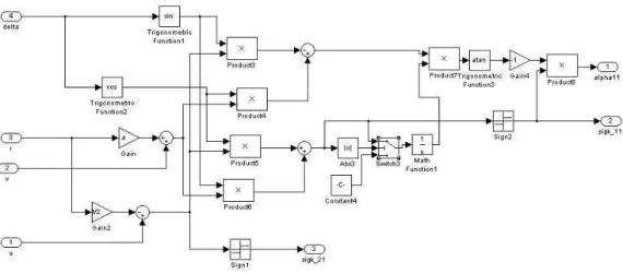
This subsystem is in turn made up of eleven subsystems (fig.3.1). We can observe on the left three subsystems in which the equations (2.1, 2.2, 2.3, 2.8, 2.9) are solved, and eight subsystems on the right in which the slip angles, the magnitudes of the wheel center speeds, and the signs of their x-components are calculated. In particular it is interesting to notice that the slip angles are not computed as in (2.12, 2.13, 2.14, 2.15), in fact we needed to improve these relations for two different reasons
1. Considering a turned wheel in particular conditions the slip angle calculated through the theoretical relation can be greater than 90 deg, and it is not correct. To un-derstand this fact we can think about two locked wheels, moving as represented in fig.3.2. The lateral forces must be the same, but without correcting the theoretical equation we work out two different slip angles, then different forces. For this reason actually we do not calculate (δ − α) (2.12 and 2.13) but (−α). The first two relations were obtained just through the analysis of the chassis motion (u, v, r), without taking into account the wheel position. On the contrary in our improved model we consider the rotation of each wheel reference frame, arriving at the following equations
Figure 3.1: Vehicle subsystem
tan (−α11) = −(u − r
t
2) sin δ + (v + ra) cos δ (u − rt
2) cos δ + (v + ra) sin δ
(3.1)
tan (−α12) = −(u + r
t
2) sin δ + (v + ra) cos δ (u + rt
2) cos δ + (v + ra) sin δ
(3.2) To take account of the position of each wheel reference frame is useful also in case we wanted to improve the tyre scheme in future. Indeed more complex models cannot
disregard the individual tyre position since the tyre motion can become too complex to analyze considering just the global vehicle reference frame (i, j, k).
2. As mentioned in the paragraph 2.2.2 a slip angle calculated by means of the the-oretical relations can represent correctly the direction of the side force only if the wheel reference frame changes depending on the x-speed direction. Nevertheless in our model we consider a “fixed” wheel reference frame, or better a reference frame rotating together with the wheel but in which the x axis keeps its initial positive di-rection independently of the x-speed didi-rection. Then we built a subsystem in which the slip angle computed through the theoretical formula is multiplied by the sign of the x-component of the wheel center speed (with respect to our “fixed” reference frame), as shown in figure 3.3.
Figure 3.3: Example of subsystem built to calculate the slip angles
In this way the direction of lateral forces is correctly represented even if the mentioned above speed changes its sign (fig.3.4).
3.1.2
Tyre Subsystem
The model is obviously provided with four of these subsystems, but since they are almost equal, we present just only one here.
This subsystem is made up of several subsystems in which the values obtained through (2.4, 2.19, 2.20 or 2.23, 2.21 or 2.24, 2.26, 2.27, 2.28) are calculated. In this block we can notice some differences in comparison with the theoretical equations.
Figure 3.4: Reference frame used to calculate the tyre forces
• The longitudinal slip k presents a problem similar to the slip angle α and, to solve it, to multiply the values worked out through the theoretical definition (2.11) by the x-speed sign would be necessary. However in our model we do not calculate k using the theoretical formula, but we compute
ˆ
k = −| Vx | −reΩ
| Vx |
To obtain the desired value, we can multiply by the Vx sign just the |Vx| that is on
the numerator (fig.3.5).
• Since we were interested in building a model that could represent the vehicle during
critical manoeuvre, we had, to calculate Fx0, to limit σ∗ at a value lower than 1.
In fact, observing (2.17) we can notice that within admissible limits for k (k ∈
[−1, +∞)), σx ∈ (−∞, 1]. However using (2.18) we can compute, for example if the
slip angle is very wide, σx values greater than 1. Then, applying the inverse formula
keq = σ
∗
1−σ∗ we can obtain keq < 0 even if σx > 0, and it obviously is not correct
Figure 3.5: First order filter subsystem
Figure 3.6: Limitation of σ∗
• To use the first order filter we preferred to multiply the equation (2.28) by |Vx|, such
a way to avoid to have a denominator that can be equal to zero (fig.3.5).
• To take into account load transfer in the “Magic Formula” created an algebraical loop which did not allow to solve the equations, and to solve this trouble a “Delay Block” was inserted in this subsystem. A “Delay Block” gives as output the value received in input a certain defined time before. We put one of them in each “Magic Formula
Subsystem”, and its input (and output) is the stiffness factor (Bx,y, see par.2.2.3).
It is simple to understand the fact that this block needs a value to give as output during first instants of simulation, for a time equal to the delay time. Obviously we
fixed this value equal to the stiffness value calculated considering Fz0 (fig.3.7). In this manner we managed to make the solver complete simulations.
Figure 3.7: Magic Formula subsystem
• The brake torque applied while the ESP is acting does not have a constant direction, but its sign depends on the sign of the wheel rotational speed. For example this fact does not occur as for the drive torque. Indeed a brake torque has every instant the direction opposite to the wheel rotational speed. To represent this phenomenon we multiply the magnitude of the brake torque, provided by the ESP subsystem, by a value obtained through the subsequent function (fig.3.8), where in abscissa we find the wheel rotational speed. This function is very similar to a “sign”. We used it in order to avoid that some problems arose during the simulations if a wheel had been close to lock. Indeed contrary to a “sign” it does not have any discontinuities and the solver can easily compute the solution.
Figure 3.8: Function used to determine the brake torque direction
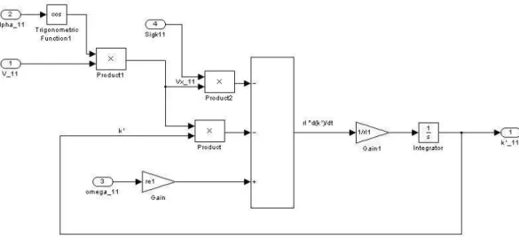
3.1.3
Engine Model
In this block we calculate the torque provided by the engine. We have the wheel rotational speeds as inputs and, by means of a switch, we can choose to use the front wheel velocities (in case of front-wheel drive car) or the rear wheel speeds (in case of rear-wheel drive car) to work out the engine rotational velocity. Clearly to determine the crankshaft rotational speed we need to know the gear and the differential transmission ratios. Giving this value in input to the “Function Block” on the right we obtain the drive torque as output. This block is very flexible in fact, defining opportunely this function it is possible to keep constant torque, constant power, otherwise using an experimental curve we can simulate for example a constant engine load condition (fig. 3.9).
If the “Function Block” represents a real torque curve the output is the torque provided by the engine in full power conditions and, to simulate the choking of gas we multiply the output by a coefficient included between 0 and 1. We inserted in this subsystem also a controller which is able to make the engine provide a torque such to keep an almost constant vehicle speed (if the engine characteristic allows this), acting on a virtual throttle pedal.
Figure 3.9: Engine subsystem
3.1.4
Haldex Coupling Model
This subsystem (fig.3.10) realizes the equations (2.10) and to represent the coupling char-acteristic (fig.2.6) we used a “Look Up Table”. The output of the “Look up Table” is multiplied by a value (controlled by an external system described in Cap 5) representing the valve position . The result is the torque going towards the front axle (if the car is normally rear-wheel drive, or vice versa) before the differential (the torque that each wheel receives depends also on the differential transmission ratio). In any case the torque trans-mitted by the “Haldex” coupling is limited at a maximum value, usually included between 2000N m and 3000N m, because a greater value can damage the drive line components. In the real coupling this safety system is realized opening a pressure relief valve but in our model we just limited the maximum value by a “Minimum Block” without simulating the valve opening. Subtracting the transmitted torque from the total torque provided by the engine (after the gear-box) we calculate the torque going towards the driving axle. Also in this subsystem, as in the “Engine Subsystem”, to choose to simulate a front-wheel drive car or a rear-wheel drive car is possible simply controlling a shift.
Chapter 4
Active Yaw Control
4.1
ESP
As already mentioned in the introduction, nowadays many cars are provided with stability control systems. Now we describe when and how these kind of devices act, focusing on the ESP and on our innovative system.
4.1.1
ESP Working Principles
The ESP is an Active Yaw Control studied in order to increase vehicle safety, avoiding excessive oversteering or understeering behavior. This system receives information from several sensors installed on the vehicle (steering wheel angle, yaw-rate, yaw-acceleration, wheel speeds, etc.), and through these signals a software is able to estimate instant by instant the car motion. Comparing the “real” estimated motion with an ideal behavior provided by software it is possible to understand if the car is behaving in a stable, foresee-able and controllforesee-able way, or if the driver is probably loosing control.
Considering for example a left-hand curve, if an excessive oversteer is detected the system
activates the front-right brake, such a way to create a negative longitudinal force (Fx12),
and in the same time to decrease the lateral force (Fy21). Both these effects contribute to
decrease the yaw-acceleration (2.3), such a way to avoid that the car begins to spin around or anyhow to prevent an undesired behavior that, if not controlled by a professional driver, can be dangerous (fig.4.1).
By a similar principle if an excessive understeer was detected the ESP would activate the rear-left brake, to generate a pro-cornering yaw moment (fig.4.1).
Figure 4.1: Effects of the ESP on vehicle motion
4.1.2
ESP Simulink Model
In our model we designed an ESP which is represented in fig.4.2. Our ESP receives as inputs: the instantaneous yaw rate, a reference yaw rate, the vehicle lateral acceleration, an estimated lateral acceleration, the front and rear drive torques, and the steer angle. Now we illustrate how these signals are obtained and afterwards we describe how our ESP processes them to recognize a dangerous situation.
4.1.3
“Reference Yaw Rate” Value
The “Reference Yaw Rate” value is one of the inputs used to decide whether to activate or not to activate the ESP. This input is worked out by the following expression
YR= r − r
ref |rref|
sign(r) (4.1)
The yaw rate (r) is a quantity that can be measured by a sensor, and rref is the reference
yaw rate.
To calculate the reference yaw rate our ESP needs, we built a “sub-model” of car. This is a “Single Track Model” ( [6], [11]) provided with linear tyres. In this case we
are allowed to use this model because it is not affected by the ESP intervention1. The
1
Actually the brake action influences the wheel speeds then ,as explained further on, the estimated ve-hicle longitudinal speed. However we can neglect this phenomenon since it proved not to have a substantial effect.
Figure 4.2: ESP subsystem
internal “sub-system” in fact just provides the reference motion we want the “real” car to follow (if necessary by means of the Active Yaw Control), but we do not apply to this any brake torque. In addition the ideal motion is surely characterized by a longitudinal speed much higher than both the side velocity and the speeds produced by the yaw rate. These conditions assure that the “Single Track Model” represents correctly the “reference vehicle” behavior.
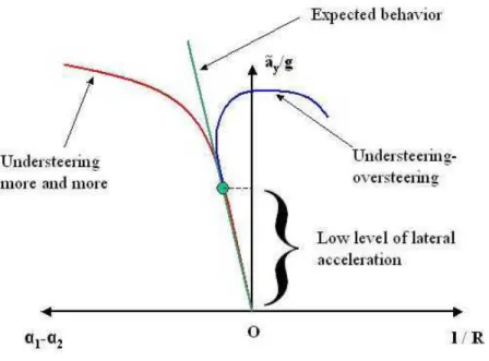
We modelled linear tyres because a non professional driver, if for example a car is understeering when the lateral acceleration is low (situation which occurs when the tyres are working in their linear zone), probably he expects a similar understeering behavior also when the lateral acceleration increases. It means that the driver is prepared for the motion that the vehicle would have if the whole tyre characteristic was linear. For these reasons he could be annoyed by a vehicle with highly non linear behavior, or for example he could be not able to control the car that suddenly becomes oversteering if the lateral acceleration exceeds a threshold value (fig.4.3). Our “sub-model” calculates the yaw-rate which the
Figure 4.3: Expected vehicle behavior in comparison with two possible real handling dia-grams
“reference car” would be going to reach in steady state conditions by the relation [6] rss= rref =
C1C2lu
C1C2l2 − mu2(C1a − C2b)
δ (4.2)
C1,2 are the cornering stiffnesses of the front and the rear axle. Whereas a linear tyre
is representative of low lateral forces, hence low lateral acceleration conditions, we are
allowed not to take into account the lateral load transfer to estimate C1,2. To evaluate
them we calculate BCDy1,2 considering the static vertical load, then using the following
relation C1,2 = 2BCDy1,2, as explained in [6].
However we have to consider that the longitudinal speed is not a value provided by sensors
on a real car, therefore to work out rref we had to find out a way to approximate it.
We observed that to estimate u we could measure just the wheel speeds, and to use the subsequent formula
uest=
re(ω11+ ω12+ ω21+ ω22)
4 (4.3)
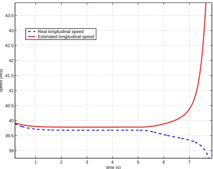
For example in fig.4.4 the real speed and the estimated speed are compared during a manoeuver that makes the car spin around because a wheel suddenly looses grip (after 5
s). We can notice that the speed value computed by (4.3) is rather similar to the real value
during the first 7 seconds, during which β2 is quite little (indicatively smaller than 10 deg).
Considering that to keep stability an ESP system must start acting within few instants after the loss of grip it is easy to understand that our estimated value can be an acceptable approximation of the longitudinal speed in order to detect a dangerous condition in time.
1 2 3 4 5 6 7 39 39.5 40 40.5 41 41.5 42 42.5 43 43.5 time (s) speed (m/s)
Real longitudinal speed Estimated longitudinal speed
Figure 4.4: Comparison between the real longitudinal speed and the estimated longitudinal speed
To estimate u some problems arise in case the ESP acts for a long time, but without succeeding in holding β in a small range. Further on we illustrate how we solved these problems.
Obviously we want to keep “YR” as close to zero as possible, in fact “YR” −→ 0 =⇒
r −→ rref. It means also to try to keep the estimated instantaneous “R” distance, defined
as the distance between the vehicle instantaneous center of velocity and the longitudinal symmetry axis of the car (fig.4.5), close to the “R” distance of the ideal trajectory. In fact,
as mentioned in [6] we can obtain the simple kinematic relation R = u
r and, considering
u ≈ uest, if r = rref also R ≈ Rest= Rref.
Unfortunately we found out that an ESP strategy based only on the “YR” value could
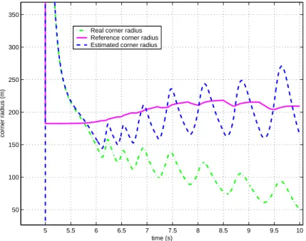
fail in particular cases, usually in oversteering conditions. In fact some simulations provided results like those shown in fig.4.6.
2
β is the body slip angle, defined as β = arctanv
Figure 4.5: Definition of “R” distance
The estimated curve radius remains quite close to the reference radius during the whole simulation, but the real radius deviates from the reference input. We also noticed that this behavior matched with a β angle decreasing more and more (fig.4.7), and when the |β|
angle was quite wide the uest began to overestimate u too much, in such a way that the
estimated car behavior differed notably from the real behavior. Clearly this fact causes an ESP action that is insufficient, and for this reason we needed to improve our system
5 5.5 6 6.5 7 7.5 8 8.5 9 9.5 10 50 100 150 200 250 300 350 time (s) corner radius (m)
Real corner radius Reference corner radius Estimated corner radius
Figure 4.6: Real, estimated and reference “R” distance in case of inefficacious ESP inter-vention
Figure 4.7: Body slip angle in case of inefficacious ESP intervention adding another parameter to control.
4.1.4
“Lateral Acceleration” Difference
The second parameter we decided to keep under control was the “AL” (Lateral
Accelera-tion) difference, defined as
AL = (˜ay − ay) sign(r) = (uestr − ( ˙v + ur)) sign(r) (4.4)
In steady state conditions ˙v is equal to zero, or in any case also during a transitory, apart from the first instants after a steering action, ˙v can be usually considered negligible with
respect to ur. Thus to hold AL close to zero means to keep uest close to u. In this way
we managed to hold β within a small range. We also want to point out the fact that,
neglecting ˙v, a dangerous oversteer matches with an AL > 0 but even if an oversteering
manoeuver is very violent, and ˙v cannot be ignored for example it is negative (considering
a left-hand curve) and it contributes to increase AL without interfering negatively on the
ESP control strategy (we deal with the ESP strategy in the next paragraph). Moreover
we found out that to control only AL could be sufficient to prevent oversteer, but we kept
4.1.5
ESP Strategy
The brake torque to apply to dominate the vehicle motion is provided by a PI controller
which arranges it to keep the two inputs (YR and AL) close to zero, as schematically
illustrated in fig.4.8. If the controller output is positive (situation corresponding to a detected understeer) the brake torque is applied to a rear wheel, if it is negative (oversteer) it is applied to a front wheel (clearly with positive sign). We select to activate the left or right brake depending on “sign(r)”. For example, referring to the front axle, we brake the left wheel if r is positive, and we brake the right wheel if r is negative. The opposite occurs with regard to the rear axle.
eYR = YR,ref− YR eAL = AL,ref− AL Mb(t) = PYReYR+ IYR Z t 0 eYRdt | {z } P IYR + PALeAL+ IAL Z t 0 eALdt | {z } P IAL (4.5)
However a normal PI controller is not suitable to represent an ESP since the ESP acts only when a really dangerous condition arises, but the PI provides an output generally different from zero every instant, that is to say it would activate the brake system con-tinuously. Then, in order to make our system more realistic, we decided to activate the brake system only in case the output provided by the controller had exceeded an upper threshold, or a lower threshold. More exactly we do not activate a brake as soon as the controller output is bigger (or smaller) than a threshold but we check that the output exceeds the limit also some hundredths of second later, before deciding to act. We created this loop in order to avoid to activate a brake when the situation does not really require an ESP intervention but somehow the PI inputs present a peak, for example because the steer angle suddenly passes from zero to a different value, hence the PI output is great. Furthermore, in some critical manoeuvres, for example if in a rear-wheel drive car the steer angle is very wide (obviously it depends on the speed), it can occur that the two inputs would need opposite outputs to be brought closer to zero. This fact causes a system
response which is unsatisfactory for both YR and AL. We decided that the most important
between the two inputs is AL. We prefer to obtain a β angle quite little, even if the car
takes the bend wider than the “reference curve”, rather than to have a car which follows a trajectory closer to the reference, but with an excessive body slip angle. This kind of motion in fact makes the driver perceive the situation as dangerous. In addition, as
men-tioned above, to consider only YR can cause a car which actually drives along a trajectory
very different from the estimated trajectory, such a way to make inefficacious the Active Yaw Control. To avoid that the controller behaves in this wrong way we multiply the
output of the PIYR controller by a coefficient between 1 and 0, which starts decreasing if
PIAL exceeds a lower threshold, following a curve like that shown in fig.4.9.
We want to point out the fact that until now we did not limit the maximum brake torque the ESP system can apply, and it is unrealistic (the ESP systems in production do not exploit the maximum longitudinal force a tyre can transfer) and it is dangerous because if the applied brake torque is excessive it causes the wheel lock. For these reasons we want to determine the maximum acceptable brake torque. Therefore the lateral load transfer is estimated using a simple linear relation (mentioned in [6]).
∆Fz1 = b ld1+ kφ1 kφ(h − d) t Y (4.6)
−900 −800 −700 −600 −500 −400 −300 −200 −100 0 −0.2 0 0.2 0.4 0.6 0.8 1 ←Table data PILA output weight coefficient
Annotations denote column breakpoints
Figure 4.9: Weight coefficient the PIYR output is multiplied by
∆Fz2 = a ld2+ kφ2 kφ(h − d) t Y (4.7)
The total side force (Y ) is calculated multiplying the lateral acceleration ay (measured
through sensors) by the vehicle mass (m). Then, we have all the elements to calculate an
approximation of Dx (2.23) (it is the peak force in pure longitudinal slip conditions) and
we multiply this value by the distance between the ground and the slip wheel axis (H) and by a safety factor (in general close to 0.5). This is the maximum brake torque applicable at a non driven wheel. Obviously an eventual drive torque affects the forces a tyre transfers to the street. To consider this fact we sum the drive torque applied to the wheel we want to brake to the brake torque previously calculated. In this way we obtain the maximum brake torque we really wish to apply. Clearly on our car we need a model of “Haldex” coupling to take into account the effects of the redistribution of torque, to estimate the drive torque.
Moreover, in order to build an ESP model as realistic as possible we created a system that checks the controller output ten times per second (in fact a real system does not receive signals from sensors continuously, and the CPU needs time to process the inputs), and it keeps the output constant during the time between two subsequent checks (obviously it may be zero).
In the end, in order to have a more realistic performance with reference to the brake torque, and to limit unrealistic peaks, for example in the vehicle speeds, due to the fact that the software calculates a numerical solution of the equations and it is negatively affected by discontinuities in the inputs, we do not use in the balance equation (2.4) the brake torque calculated as mentioned above, but we filter it by means of a simple first order filter, which equation is
Kd˜x
dt + ˜x = x (4.8)
Chapter 5
Redistribution of Torque
In our model we analyzed the effects of the engine torque redistribution between rear and front axle to study the feasibility of a new stability control system, or to improve perfor-mance of traditional ESP’ s. The natural oversteer-understeer of a vehicle is due to many different factors: vertical load distribution between front and rear axle, tyre characteristic, engine torque flow, suspension geometry and stiffness, etc. In particular the drive torque flow, on account of the typical tyre behavior, makes the vehicle inclined to be oversteering if the torque is directed towards the rear axle. On the other hand a front-wheel drive car is inclined to be understeering. This fact does not mean that necessarily a front-wheel drive vehicle is oversteering and the contrary for a rear-wheel drive car, by reason of the several factors affecting the vehicle behavior. However considering two cars which are different just in the drive torque distribution (as we did in our research) we can say that the front-wheel drive vehicle is “more understeering” than the rear-wheel drive car (but for example both of them can be oversteering). In order to give an intuitive explanation of the reason of the different behavior we illustrate a simple, but not rigorous demonstration.
We consider a “Single Track Model” (5.1) with linear tyres ( [6], [11]), in order to schema-tize a front-wheel drive car and a rear-wheel drive car, both with the same characteristic dimensions.
Starting from the balance equations we can calculate the curve radius the car drives along in steady state conditions
Rss= u rp = 1 δ(l − ( C1a − C2b C1C2 )mu 2 l ) 1 (5.1) 1
This equation (as remarked in [6]) is valid for a rear-wheel drive car, but can be acceptable to model a front-wheel drive car if the steer angle is small enough, so in the following demonstration we accept this simplification.
Figure 5.1: “Single Track Model” scheme
C1,2 are the equivalent cornering stiffnesses of the front and rear axles. As explained in
the second chapter the longitudinal forces transferred by a tyre influence the lateral forces, but the linear model does not take this fact into account. We can imagine to approximate combined slip conditions reducing the cornering stiffness, multiplying it by a positive factor lower than 1 ((1 − ε) and (1 − γ)). Considering a car equipped with the same type of tyre in the front and in the rear axle, producing an axle cornering stiffness equal to C we obtain (with the subscript f we refer to the front-wheel drive car and with the subscript r we refer to the rear-wheel drive car)
Rss,f = u rp = 1 δ(l − ( C(1 − ε)a − Cb (C(1 − ε))C ) mu2 l ), 0 < ε < 1 (5.2) Rss,r = u rp = 1 δ(l − ( Ca − C(1 − γ)b C(C(1 − γ)) ) mu2 l ), 0 < γ < 1 (5.3)
Considering for both the cars the same longitudinal speed (u) and the same steer angle
(δ), we calculate Rf − Rr, and we achieve the following result
Rf − Rr = mu2 l (− C(1 − ε)a − Cb C2(1 − ε) + Ca − C(1 − γ)b C2(1 − γ) ) = = mu 2 l ( b(1 − γ)ε + a(1 − ε)γ C(1 − ε)(1 − γ) ) (5.4)
In (5.4) both the numerator and the denominator are greater than zero, then Rf−Rr >
means Rf > Rr, that is to say the front wheel drive car drives along a wider bend than the rear-wheel drive car.
We can try to understand the reason of the different behavior also during a transitory, for example considering a manoeuvre in which the steer angle follows a step function with null initial value. In fact when it passes from zero to another value only the front wheel
has a slip angle different from zero (exactly equal to the steer angle), but α2 = 0, hence
Fy2 = 0. For the balance equation
J ˙r = Fy1a − Fy2b (5.5)
We obtain (giving the two cars the same steer angle also in this case) a front wheel-drive car that has a yaw acceleration lower than the rear-wheel wheel-drive car. It means that, supposing the two cars running at the same longitudinal speed, at least during the first
instants Rf will be wider than Rr.
Our idea was to try to transfer torque to the front axle in case of excessive oversteer, and contrary to provide torque to the rear axle if an excessive understeer is detected. This system cannot replace an ESP system completely because for example if it is applied on a front-wheel drive car, it can be able only to correct understeer, but to correct an oversteering behavior a traditional ESP remains necessary. The opposite occurs for a rear-wheel drive vehicle.
5.1
Drive Torque Control
Since the vehicle we modelled is supplied with an “Haldex” coupling we can only intervene on the internal valve position to govern the engine torque flow.
5.1.1
Controller
To control the valve we used the same quantities as in the ESP. If the PI controller output exceeds a threshold value we close completely the valve, therefore we transfer the maximum possible amount of torque (depending on the working point on the coupling characteristic), otherwise we keep the valve open, and no torque is transferred (fig.5.2). The threshold magnitude for the valve controller is lower than the correspondent value for the ESP. Initially we want to control the car motion acting on the distribution of torque, and only if this intervention is not effective we activate the brake system. As long as possible in fact we
want to avoid to apply a brake torque. The simulations confirm that the ESP intervention is very powerful but also uncomfortable, and it makes the vehicle performances worse.
Figure 5.2: “Redistribution of Torque” controller subsystem
We prefer to use a control which opens or closes completely the valve without any possible intermediate position because the redistribution of torque exploits an amount of drive torque, and whereas its value is not usually very big (in comparison for example with the brake torque applied by the ESP), the whole available torque must be applied to obtain performances as strong and quick as possible, without risking to overcompensate the undesired behavior.
Chapter 6
Rear-Wheel Drive Car simulations
In this chapter we present the results provided by the simulations, with regard to a rear-wheel drive car, in the next chapter we deal with a front-rear-wheel drive car. In all the simulations we impose open-loop steer angles; we define the steer functions before running the simulations, and they are not affected by the vehicle motion. Therefore the driver in-puts depend on the instantaneous vehicle behavior whereas man-car-external environment constituted a closed-loop system.
In this report we refer to a vehicle equipped with tyres which size is 195/65-R15. The vehicle model we analyzed to define the Active Yaw Control set-up was provided with a set of tyre parameters obtained testing this tyre. We simulated also a car supplied with tyres 205/55-R15, without changing the PI controller, in order to understand if an ESP and redistribution of torque controller allows to obtain good results even if its set-up is at first developed for another type of tyre. Some simulations regarding the car provided with the sport tyres are illustrated in the “Appendix A” and in the “Appendix B”. The M-file in which are included the tyre and car parameters is reported in “Appendix C”.
6.1
High Speed A
The first simulation illustrates condition in which the driver wants to drive along a too sharp curve, considering the car speed. The speed in fact is, before starting the cornering
manoeuvre, close to 55 m
s (almost 200
km
h ), and the steer angle follows a step function,
represented in fig.6.1. The final value is 0.5 deg, and supposing a steer transmission ratio equal to 1:20, it corresponds to an angle, applied by the driver to the steering wheel, equal to 10 deg.
0 1 2 3 4 5 6 7 8 9 10 −0.1 0 0.1 0.2 0.3 0.4 0.5 0.6 time (s)
steering angle (deg)
Steering angle
Figure 6.1: Steer angle function
with the ESP, and provided with the “Haldex” coupling. We tried also to simulate the combined effects of the ESP and redistribution of torque but in that case the ESP system does not act.
Analyzing the trajectories the cars drive along (fig.6.2) we can understand that our stability control detects an oversteering manoeuvre. The trajectories which the two cars provided with the stability systems follow in fact are wider than the bend driven along by the uncontrolled vehicle. However we can realize better the real effect of the stability systems comparing the “R” distance and the body slip angles (β) in the three cases (fig.6.3 and fig.6.4)
If the car is not provided with any Active Yaw Control it looses stability and it spins around. We can understand this fact since the “R” distance decreases too much, approach-ing zero, and |β| becomes bigger and bigger. Observapproach-ing fig.6.3 we want to point out that using a stability system we manage to keep an average curve radius close to the reference radius, but we do not reach a stable steady state condition. Also the β angle remains quite small, and it does not exceed -10 deg (if the body slip angle becomes lower we decided to consider the simulation failed because in a car following that motion a driver would not feel safe). In order to achieve this goal we activate the brake system and the central coupling in the way shown in fig.6.5, 6.6, 6.7.
300 320 340 360 380 400 420 440 460 480 0 5 10 15 20 25 30 35 40 45 distance (m) distance (m) Redistribution ESP NO Control
Figure 6.2: Trajectories driven by the three vehicles
5 5.5 6 6.5 7 7.5 8 8.5 9 100 200 300 400 500 600 time (s) corner radius (m) Redistribution Reference radius ESP NO control Figure 6.3: “R” distances
5 5.5 6 6.5 7 7.5 8 8.5 9 −60 −50 −40 −30 −20 −10 0 time (s) beta (deg) Redistribution ESP NO Control
Figure 6.4: Body slip angle
5 5.5 6 6.5 7 7.5 8 8.5 9 0 100 200 300 400 500 600 700 800 time (s) Mb 12 (N*m)
5 5.5 6 6.5 7 7.5 8 8.5 9 0 50 100 150 200 250 300 350 400 450 500 time (s) Mb 21 (N*m)
Figure 6.6: Brake torque applied to the rear inner wheel
4.5 5 5.5 6 6.5 7 7.5 8 8.5 9 0 0.1 0.2 0.3 0.4 0.5 0.6 0.7 0.8 0.9 1 time (s)
valve (1 closed; 0 open)
We want to remark the fact that both an ESP action (with regard to the front outer brake (fig.6.5)) and a redistribution of torque action (fig.6.7) match with a “R” distance and a β angle that increases. In reference to the rear inner brake (fig.6.6) we can notice that it is never activated simultaneously with the front brake, and the brake torque is lower and lower during the simulation, and after few time it becomes null. The effect of this braking action is to damp oscillations that the ESP would trigger during the first instants of the manoeuvre if it acted on only one brake.
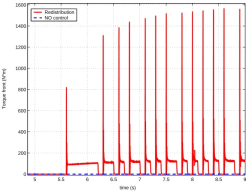
The intervention of the “Haldex” system causes a torque directed towards the front axle which is reported in fig.6.8 (this is the torque provided by the coupling, before the differential gear box).
5 5.5 6 6.5 7 7.5 8 8.5 9 0 200 400 600 800 1000 1200 1400 1600 time (s) Torque front (N*m) Redistribution NO control
Figure 6.8: Drive torque provided to the front axle
Except for the first instants after the valve closing, during which we have very high peaks, that in any case decrease so quickly not to have significant effects on tyre perfor-mances, the car reaches a condition in which the amount of transferred torque is almost constant while the valve is closed.
In this first simulation we illustrate also the tyre performances, to stress the effects of this two stability systems on the forces which the car motion is due to.
Without using any control system we can notice the fact that the forces transmitted by the inner tyres become zero after almost 7 s (fig.6.11, 6.13, 6.15), and it means that the
4 4.5 5 5.5 6 6.5 7 7.5 8 8.5 9 0 50 100 150 200 250 300 350 400 450 500 time (s) Fx 11 (N) Redistribution ESP NO control
Figure 6.9: Longitudinal force transferred by the front inner tyre
4.5 5 5.5 6 6.5 7 7.5 8 8.5 9 −3000 −2500 −2000 −1500 −1000 −500 0 500 1000 time (s) Fx 12 (N) Redistribution ESP NO control
4.5 5 5.5 6 6.5 7 7.5 8 8.5 9 −800 −600 −400 −200 0 200 400 600 800 1000 time (s) Fx 21 (N) Redistribution ESP NO control
Figure 6.11: Longitudinal force transferred by the rear inner tyre
4 4.5 5 5.5 6 6.5 7 7.5 8 8.5 9 −200 0 200 400 600 800 1000 time (s) Fx 22 (N) Redistribution ESP NO control
4 4.5 5 5.5 6 6.5 7 7.5 8 8.5 9 0 200 400 600 800 1000 time (s) Fy 11 (N) Redistribution ESP NO control
Figure 6.13: Lateral force transferred by the front inner tyre
5 5.5 6 6.5 7 7.5 8 8.5 9 0 500 1000 1500 2000 2500 3000 3500 4000 4500 5000 time (s) Fy 12 (N) Redistribution ESP NO control
4 5 6 7 8 9 0 100 200 300 400 500 600 700 800 time (s) Fy 21 (N) Redistribution ESP NO control
Figure 6.15: Lateral force transferred by the rear inner tyre
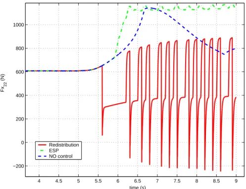
4.5 5 5.5 6 6.5 7 7.5 8 8.5 9 0 500 1000 1500 2000 2500 3000 3500 4000 4500 time (s) Fy 22 (N) Redistribution ESP NO control
vertical load acting on these wheels is null. On the contrary we can observe the side forces transferred by the outer tyres which reach very high values on account of the considerable vertical load and because the slip angles are surely quite wide (the global effect of this set of force is in fact a car which spins around).
With regard to the car provided with the central coupling we can see the effects of the redistribution of torque on the forces. Obviously the longitudinal forces due to the front wheels increase (fig.6.9 and fig.6.10) and contrary the forces transmitted by the rear wheels decrease (fig.6.11 and fig.6.12) when this system is intervening. While the coupling is acting we obtain four tyres which produce longitudinal forces different from zero and both the inner and the outer wheels of the same axle transfer almost the same force (not exactly the same because of the different vertical load which does not allow the inner wheels to exploit the whole drive torque). The global effect is in any case positive to decrease the yaw rate, compared to the situation occurring without using any stability control system. After few seconds only one outer wheel transmitted a significant longitudinal force (fig.6.12), and it causes a positive yaw acceleration. The lateral forces have a more constant value in the previous case, and the effect of the ellipse of grip is clear, in fact when a longitudinal force increases, in the same time the corresponding lateral force decreases (see for example fig.6.9 and fig.6.13). In this way, when we close the valve we decrease the front lateral forces and we increase the rear lateral force, and this fact causes a change in yaw acceleration.
The vehicle which uses the ESP keeps stability exploiting the tyre forces in a different manner. In fig.6.10 and in fig.6.14 we can observe the effects of the brake torque respectively on the longitudinal and lateral force. The longitudinal force reaches significant negative peaks and, being applied on the front outer wheel, it produces a contra-cornering yaw moment. In the same time, when we apply the brake torque the lateral force decreases on account of the tyre behavior in combined slip conditions, and also this fact contributes to avoid oversteer. The performance of the rear inner tyre (fig.6.11 and fig.6.15) is very influenced by the oscillating vertical load and for this reason it presents a not very regular trend both on longitudinal and lateral forces.
In fig.6.17 the yaw acceleration in the three different cases is presented. The graph displays that the non controlled vehicle has a positive yaw acceleration during the whole simulation, hence the yaw rate is continuously increasing. In particular during the last instants the acceleration has a a very high positive slope and it reaches a very high peak. At that moment the car is totally out of control and it is starting spinning around.
4 6 8 0 0.1 0.2 0.3 0.4 0.5 time (s)
Yaw accel. (rad/s
2) 5 6 7 8 9 0 0.1 0.2 0.3 0.4 0.5 time (s)
Yaw accel. (rad/s
2) 5 6 7 8 9 −1 −0.8 −0.6 −0.4 −0.2 0 0.2 0.4 0.6 time (s)
Yaw accel. (rad/s
2)
NO control Redistribution ESP
Figure 6.17: Vehicle yaw acceleration in the three different cases
acceleration oscillate around zero, to limit the yaw rate. The redistribution of torque produces a more regular performance than the ESP, in fact the positive and negative peaks remain closer to zero. This fact is positive because, as we can observe in fig.6.3, the bend radius does not deviate from the reference radius as much as using the ESP. However considering that we are transferring the maximum amount of torque allowed by the central coupling it means that using the brake system it is possible to create a much stronger contra-cornering yaw moment.
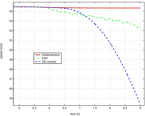
Now we want to analyze the effects of these systems on the car performance. In all the simulations we used the virtual pedal gas trying to keep constant speed (see par. 3.1.3), and the redistribution of torque system exhibited a good potential also in order to maintain an high velocity. In fig.6.18 we can see that, since the ESP acts on the brake system it obviously makes the vehicle slow down, contrary to the redistribution of torque system, which allows to keep an almost constant speed.
In the end of the simulation the difference between the two speeds of the center of
gravity (VG =
√
u2+ v2) is almost 2 m
s, and even if it is not a significant difference for a
normal car, it could be very important for a competition vehicle.
In reference to the vehicle comfort in fig.6.19 we compare the center of gravity
5 5.5 6 6.5 7 7.5 8 8.5 9 45 46 47 48 49 50 51 52 53 54 time (s)
speed (m/s) RedistributionESP
NO control
Figure 6.18: Center of gravity speed
4 4.5 5 5.5 6 6.5 7 7.5 8 8.5 9 −2 −1.5 −1 −0.5 0 0.5 1 time (s) long. acc. (m/s 2) Redistribution ESP
level of longitudinal acceleration the passengers are subjected to. Also in this case we want to remark the negative effect of the strong action of the ESP, which produces a much more variable level of acceleration than the redistribution of torque, with very high positive and negative peaks. For this reason the ESP intervention is surely more annoying and uncomfortable than the “Haldex” coupling action.