Chapter 2
Efficient Evaluation of the Matrix Elements in the Context of the MoM
A novel technique is developed for an efficient derivation of MoM matrix elements for scattering problems. The proposed method is intended for overcoming some of the limits of the conventional MoM formulation, leading to a robust as well as efficient MoM-based approach. The Chapter will begin by introducing the basic formulation along with the closed-form expressions utilized to describe the fields radiated by the employed basis functions. Both the EFIE and the CFIE will be solved through the method for deriving the current distribution and the fields scattered by conducting and dielectric bodies. Some numerical examples validating the accuracy at low frequencies as well as the numerical efficiency of the proposed technique in comparison to conventional MoM formulation are included.
2.1. Limitations in the conventional MoM formulation
Formulating integral equations via the use of the Green’s function is a well-established and universally accepted method [18], [20], [51], [52], which has been a staple for CEM problems in the past. Potential theory as well as all the formulations based on it are on solid footing and related matters as the numerical treatment of the GFs’ singularities have been researched very thoroughly over many decades. However, some deficiencies related to the conventional MoM formulation cannot be overcome by using the methods that have already been well developed.
On the basis of our experience with the conventional Green’s-function-based MoM formulation, we can identify the following areas of concern:
i Dealing with singular and hypersingular behaviour of the Green’s function when generating the MoM matrix elements
ii Handling thin wires and/or sheets, with or without finite losses
iii Dealing with the low-frequency breakdown problem introduced by the dominance of the scalar potential term over the vector potential as the frequency approaches zero
iv Accurately modeling multi-scale geometries
v Deriving a universal approach for PEC, dielectric and inhomogeneous bodies
vi Accurately integrating the Green’s function for curved geometries
The objective of this chapter is to introduce an approach that circumvents some of the issues listed above. In particular, the proposed technique will be demonstrated to be able to bypass the numerical treatment of the GF’s singularities. Furthermore, since the formulation deals with the electric fields generated by the basis functions directly, as opposed to vector and
scalar potentials typically employed in the conventional MoM formulation, the so-called ‘low frequency’ problem, which plagues the latter owing to the presence of the 1/ω factor in the scalar potential term, is no longer a concern in the presented technique, and a uniform formulation can be employed for the entire frequency range without having to resort to special basis functions.
2.1.1. Low-frequency breakdown
Moment method solutions of the electric-field integral equation using RWGs suffer from the so-called low-frequency breakdown. As a consequence of the decoupling of the electric and magnetic fields in Maxwell’s equations at zero frequency, their numerical solution at low frequencies is plagued with numerous problems. Also, the electric and magnetic fields become curl free at zero frequency outside the source region:
0 0, lim , 0 E H J E J j E ω ε ρ ω µ → ∇ × = ∇ × = ∇ ⋅ = = ∇ ⋅ ∇ ⋅ = (2.1)
This decoupling of the electrostatic and magnetostatic fields manifests itself in the current by separating into a solenoidal (divergence-free) and a complementary, irrotational (curl-free) component. At zero frequency the two components decouple completely, that is the divergence-free current produces a magnetic field while the irrotational one gives rise to an electric field. Therefore, the current undergoes a natural Helmholtz decomposition [53]. It is apparent from (2.1) that the curl-free current requires a divergence that goes to zero with vanishing frequency to produce a physically finite charge. Therefore, J=Jirr+Jsol
where the irrotational component Jirr vanishes with ω as it tends to zero. It is important to underline that no such frequency scaling is required for the solenoidal component Jsol.
Due to the diverse frequency dependence of the two components of the current with vanishing ω, a working numerical method needs to account for this Helmholtz decomposition. This has been achieved by the loop-tree and the loop star method in the contest of iterative-solvers convergence [28], [29].
When solving Maxwell’s equations via the potential method, the following expression for the produced electric fields arises:
scat
E = −j Aω− ∇φ (2.2)
in which the scalar potential φ represents the contribution from the charge ρ while the vector potential A that from the current J.
When the electric field integral equation is solved through the MoM with rooftops or RWG [28] basis functions, the contribution from the vector potential to the impedance matrix becomes much smaller than that of the scalar potential as the frequency approaches zero.
2.1.2. Numerical treatment of the Green’s functions singularities 31
This, if the frequency scaling of the curl-free component of the current is not adjusted as mentioned above.
This can be additionally inferred by studying this integral representation:
( ) ( , ) ( ) 1 ( , ) ( ) s S s S E r j G r r J r dS G r r J r dS j ωµ ωε ′ ′ = − ′ ′ ′ − ∇ ⋅
∫
∫
(2.3)Due to the finite machine precision, the first term (contribution from the vector potential) will be lost during the numerical process with vanishing ω. Moreover, the second term in (2.3) has a null space because of its divergence operator. This makes the impedance matrix nearly singular and difficult to invert at low frequencies [28], [29]; that is the loss of the contribution from the vector potential makes the solution inaccurate.
These problems can be overcome, in the context of iterative solvers, by introducing the loop-star and loop-tree decompositions [28]-[34]. These basis functions separate the contributions from the vector and scalar potentials in the impedance matrix. This way, the contribution from the vector potential is preserved in comparison to that of the scalar potential, the matrix is no longer nearly singular and the solutions are much more accurate.
The use of loop-star or loop-tree basis followed by frequency normalization, though, solves the problem of having to deal with singular matrices partially at very low frequencies. The matrix, in fact, still results ill-conditioned and if an iterative solver is used, the iteration count is usually very large and may even diverge for some problems.
2.1.2. Numerical treatment of the Green’s functions singularities
The filling of the impedance matrix for problems involving the use of the conventional potential formulation, is a computational expensive process.
By considering as an example the numerical solution of the Combined Field Integral Equations though the MoM:
[
]
[
]
1 2 1 2 1 2 1 2 1 2 1 2 1 2 1 2 ( ) ( ) ( ) ( ) ( ) ( ) ( ) ( ) ( ) ( ) ( ) ( ) ( ) ( ) i t t i t t F r F r E r j A r A r V r V r A r A r H r j F r F r U r U r ω ε ε ω ε ε = + + ∇ + ∇ + ∇ × + ′ ′ = + + ∇ + ∇ − ∇ × ′ + ′ (2.4)Testing equations (2.4) with testing functions
{ }
Bn yields: 1 2 1 2 1 2 1 2 , ( , ) ( , ) , ) i m m m m F F E B jω
A A B V V B Bε
ε
〈 〉 = 〈 + 〉 + 〈 ∇ +∇ 〉 + 〈∇× + 〉 ′ ′ (2.5) 1 2 1 2 1 2 1 2 , ( , ) ( , ) , ) i m m m m A A H B jω F F B U U B B ε ε 〈 〉 = 〈 + 〉 + 〈 ∇ +∇ 〉 + 〈∇× + 〉 ′ ′ (2.6)on surface of the generic scatterer S.
As previously shown in the last section of Chapter 1, the vector and scalar potential integrals for the example at hand take the following form:
, , ( ) 1 ( ) ( , ) ( ) 4 n n c i m n n i m i m n T T A B r G r r dS r F
π
+ − ± ± ± + ′ ′ ′ =∫∫
= (2.7) , , ( ) 1 ( ) ( , ) ( ) 4 n n c i m n s n i m i m n T T B r G r r dS rφ
ψ
π
+ − ± ± ± + ′ ′ ′ ′ =∫∫
∇ ⋅ = (2.8) , , ( ) 1 ( ) ( , ) ( ) ( ) 4 2 m n n m i m n m n i m i m n m T T T l P B r G r r dS r dS r Q A ±ρ π + − ± ± ± ± ± + ′ ′ ′ ′ ′ = ⋅ ×∇ = ∫∫
∫∫
(2.9) where: ( , ) i jk R i m e G r r R ± − ± ± ′ = (2.10) 3 ( , ) ( )(1 ) ( ) i jk R i m m i e G r r r r jk R R ± − ± ± ± ± ′ ′ ′ ∇ = − + (2.11) and R |rm r | ±= ±−′represents the distance between the source and the testing basis functions. The reaction integrals arising from the curl of the vector potentials (2.9), involve the integration of the gradient of the Green’s functions. In particular, when the field point is in the vicinity of the source, a numerical intensive process is required to accurately evaluate the reaction integrals for the impedance matrix elements owing to the singularity of the Green’s functions at the source point.
The dynamic potential integral relative to the linear nodal RWG function Ni (i = 1, 3) can be
expressed as follows:
( ) ( , )
i anl num
T
2.1.2. Numerical treatment of the Green’s functions singularities 33 with 1 ( ) anl i T I N r dT R ′ ′ =
∫
(2.13) 1 ( ) jkR num i T e I N r dT R − − ′ ′ =∫
(2.14)Integral (2.14) can be integrated numerically, by using Gaussian quadrature formulas [54], since its integrand is bounded for every observation point:
0 1 lim jkR R e j R − → − = − (2.15)
while integral (2.13) requires analytical evaluation [26].
Similarly, when the kernel is the gradient of the scalar Green’s function, the potential integral can be seen as a summation of an integral evaluated analytically Ianl
∇ and num I∇ to be integrated numerically: ( ) ( , ) i anl num T N r′∇G r r dT′ ′=I∇ +I∇
∫
(2.16)which take the form:
1 ( ) anl i T I N r dT R ∇ = ′∇ ′
∫
(2.17) 1 ( ) jkR num i T e I N r dT R − ∇ = ′∇ − ′ ∫
(2.18)2.2. Fields radiated by a rectangular basis function
In this section, a novel numerical technique is applied to compute the matrix elements in the context of the Method of Moments (MoM). The method is based on the concept of bypassing the use of the potential formulation to connect the currents with the produced fields. For this purpose, the fields radiated by sinusoidal current distributions residing on rectangular basis functions are expressed in a closed-form.
Given the particular expressions for the fields which are generated by spherical wave sources with fixed locations [55], the testing procedure can be carried out directly on the surface of the basis avoiding the numerical treatment of singularities as would happen by employing conventional MoM formulation. Furthermore, since the use of the potential formulation in deriving the fields is bypassed, the matrix doesn’t suffer from frequency scaling and can be efficiently inverted in the low frequency regime.
2.2.1. Closed form expressions for the fields radiated by a sinusoidal current
distribution
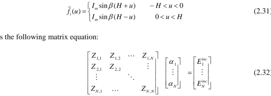
Consider a wire structure extending along the z-axis, in a spherical coordinate system as shown in Fig. 2.1.
Figure 2.1. Geometry for fields near the antenna.
Relating to the figure, the following relations will hold:
(
)
(
)
(
)
2 2 2 2 2 2 2 1 2 2 y z r y H z R y H z R y h z R + = + + = + − = + − = (2.19)2.2.1. Closed form expressions for the fields radiated by a sinusoidal current distribution 35
Assuming a sinusoidal distribution of current on the wire:
(
H h)
I
I= msinβ − (2.20)
the expression for vector potential at point P will be:
(
)
(
)
+ + − =∫
∫
− − − H H R j R j m z dh R e h H dh R e h H I A 0 0 sin sin 4 β β β β π µ (2.21)Through simple algebraic manipulations [55], the magnetic field strength at point P lying in the y-z plane can be expressed as:
( ) ( ) ( ) ( ) 0 0 0 0 8 z x H j R h H j R h j H j H m j R h j R h j H j H H H A H H y I e e H e dh e dh j y R y R e e e dh e dh y R y R φ β β β β φ β β β β µ µ π − + − − − − − − + − − − ∂ = − = − ∂ ∂ ∂ = − − ∂ ∂ ∂ ∂ + ∂ − ∂
∫
∫
∫
∫
(2.22)Given the current distribution to be sinusoidal, the integrands in (2.22) turn out to be perfect differentials. Integrating and summing up all terms yields for magnetic field strength:
− + − = − − − y He y e y e j I H r j R j R j m β β β φ π 2cosβ 4 2 1 (2.23)
The E-field can be obtained by recalling the H-field in free space:
H j E= ∇× ωε 1 (2.24)
In the y-z plane:
(
φ φ)
ωε( )
φ ωε H j y y yH j Ez z ∂ ∂ = × ∇ = 1 ˆ 1 (2.25)(
φ φ)
ωε( )
φ ωε H j z H j E y y ∂ ∂ − = × ∇ = 1 ˆ 1 (2.26)Substituting the expression for Hφ into (2.25), (2.26) yields: 1 2 1 2 2cos 4 j R j R j r m z I e e e E j H R R r β β β η β π − − − = − + − (2.27) 1 2 1 2 2 cos 4 j R j R j r m y I z H e z H e z H e E j y R y R y r β β β η β π − − − − + = + − (2.28)
and rewriting the expression for magnetic field strength:
(
1 2 2cos)
. 4 j R j R j r m I H j e e H e y β β β φ= π − + − − β − (2.29)Equations (2.27-2.29) give the electric and magnetic field strengths both near to and far from an antenna carrying a sinusoidal current distribution.
The first two terms of the parallel component (2.27) can be interpreted as two spherical waves of equal amplitude originating from the two ends of the wire [55]. The third term represents a wave originating at the centre of the wire whose amplitude depends upon H. The above expressions can be used to solve a wire scattering problem through the MoM. Consider a plane wave at the operating frequency of 10 GHz, incident upon a z-directed, λ/2 in length PEC wire, which measures λ/80 in diameter. Consider the wire is partitioned into 9 overlapping regions, λ/10 in length (Fig. 2.2).
A sinusoidal variation of the current over a short length (typically ≤ λ/10) is closely equivalent to a triangular distribution on the dipole. Therefore, if each partitioning segment is intended as a source wire carrying a sinusoidal current distribution, expressions (2.27-2.29) can be used to calculate the scattered fields.
Figure 2.2. Perfectly conducting wire λ/2 in length partitioned into 9, λ/10 segments.
The total tangential electric fields should be zero on the surface of the wire. It is made up of the contributions from all the source dipoles, located at the wire centre, radiating on the wire surface S and the incident plane wave at the wire surface. Testing the boundary equation:
tan tan
( ) ( )
s i
2.2.1. Closed form expressions for the fields radiated by a sinusoidal current distribution 37
with testing functions:
sin ( ) 0 ( ) sin ( ) 0 m i m I H u H u f u I H u u H β β + − < < = − < < (2.31)
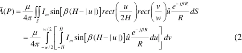
yields the following matrix equation:
1,1 1, 2 1, 1 1 2,1 2, 2 ,1 , N inc inc N N N N N Z Z Z E Z Z E Z Z α α = (2.32) where inc i
E represents the field incident at i-th dipole location, αi the generic current weight
coefficient to be derived. The generic impedance matrix element is expressed as:
( ) ( ) ( ) , 1 1 ( ) M N j i i i j n m m m n Z E R f = = =
∑∑
(2.33)where N represents the number of radiating wires, M the number of observation points for each segment and ( )j
n
E the field radiated from j-th source at i-th segment location.
By solving the above system of equations the following numerical results are obtained for the current distribution on the wire (Fig. 2.3(a)) and the scattered near fields (Fig. 2.4).
(a) (b)
Figure 2.3. Current distribution on the wire derived through conventional MoM and our method (a); the accuracy is tested by increasing the number of samples used for the discrete integration (b).
(a) (b)
Figure 2.4. Amplitude (a) and phase (b) distributions of the fields scattered by a λ/2 in length PEC wire along y (x=0, z=0). A plane wave propagating along y with a z-polarized E-field is incident on the structure.
A good correspondence is achieved between conventional MoM and the proposed technique for the current distribution and the fields scattered by the analyzed structure. The accuracy can be enhanced by employing an increased number of sampling points for the testing functions (Fig. 2.3(a)).
2.2.2. Fields radiated by a rooftop basis function
A current distribution, piecewise-sinusoidal along the uˆ direction and uniform along vˆ, over a rectangular domain (Fig. 2.5) can be represented as:
[
]
( , ) sin ( | |) 2 u m u v J u v I H u rect rect H w β = − (2.34)where 2H and w are the patch dimensions along uˆ and vˆ respectively.
2.2.2. Fields radiated by a rooftop basis function 39
The vector potential of (2.34) at point P can be expressed as:
[
]
ˆ ( ) sin ( | |) 4 2 j R m S u v e A P I H u rect rect u dS H w R β µ β π − = − ∫∫
[
]
/ 2 / 2 ˆ sin ( | |) 4 w H j R m w H e I H u u du dv R β µ β π − − − = − ∫ ∫
(2.35)where β represents the propagation constant and R the distance between the source and generic observation point P. The computation of the integral in (2.35) can be simplified, provided that the current does not vary significantly along the transverse direction vˆ:
[
]
ˆ ( ) sin ( | |) 4 H j R m H I e A P w H u u du R β µ β π − − =∫
− (2.36)which represents the potential associated to a uˆ−oriented straight dipole carrying a sinusoidal current distribution, multiplied by the rooftop width w. Therefore, since the radiated fields are expressed in terms of A, the field produced by a rooftop-like current distribution can be seen as that radiated by a straight dipole, multiplied by the rooftop width
w (Fig. 2.5) [56], [57].
In the process of employing the method for the solution of the scattering from a flat plate, the geometry is first partitioned into rectangular patches overlapping in the uˆ and vˆ directions (Fig. 2.6).
Figure 2.6. Flat conducting sheet partitioned via overlapping ˆu− and ˆv − directed rectangular basis
The parallel and perpendicular components of the fields produced by the sinusoidal basis functions are calculated through (2.27), (2.28). The summation of the tangential components of the scattered and incident fields has to vanish on the surface S of the perfect conductor. Only the parallel contribution will concur to the uˆ−uˆ and vˆ−vˆ impedance matrix field interactions, while the perpendicular contribution will have effect for uˆ−vˆ, vˆ−uˆ field interactions calculation only (Fig. 2.7).
(a) (b)
Figure 2.7 Scheme co-planar for ˆu− directed bases radiating over ˆu − directed (a) and for co-planar
ˆ
u− directed bases radiating over ˆv − directed.
The system of equations is built as in (2.32), with the generic impedance matrix element defined as:
(
, , ,)
1 ( ) ( ) ( ) M ij j i i j i m i m i m m m S Z E R f dS E R f R S = =∫∫
⋅ =∑
⋅ ∆ (2.37) where f Ri( )i represents testing function (2.31) evaluated at field points Ri
and E R j( )i is the field contribution along the test base direction:
1 2 0 1 2 2cos 4 j R j R j r m j I e e e E H R R r β β β β β πωε − − − − = + − (2.38) 1 2 0 1 2 2 cos 4 j R j R j r m I u H e u H e u H e E j v R v R v r β β β β β πωε − − − ⊥ − + = + − (2.39)
It is useful to underline that field expressions (2.38), (2.39), represent spherical waves originating at three well defined locations (top, bottom and wire centre). Therefore, all the observation points including those for self-term calculation can be located right on the patch surface (Fig. 2.8), avoiding numerical treatment of the singularity.
2.2.3. Generalized field expressions 41
surfaces and in the near field region we can improve the accuracy by employing an increased number of radiating dipoles as well as testing points when the separation distance between the basis and testing functions is below a threshold value.
Figure 2.8. Scheme for source and test sinusoidal bases with equivalent radiating dipole and observation points.
2.2.3. Generalized field expressions
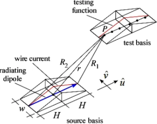
The formulation can be generalized to handle either a two- or three-dimensional structure, discretized by using arbitrarily oriented patches in space (see Fig. 2.9).
This is done by considering two independent monopoles discretizing the two half-patches of the basis function as depicted in Fig. 2.10(b). The radiating dipole representing the basis function is in general a bent wire with its two branches oriented along directions uˆ+ and uˆ−
(see Fig. 2.10(a)) arbitrary that can be. The expressions for the radiated fields can be derived by evaluating the two integrals from 0 to H1 and from –H2 to 0 (2.22) and summing up the two contributions separately.
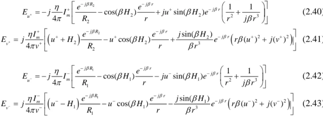
The following expressions read for the parallel and perpendicular components of the electric fields radiated by uˆ+− and uˆ−−directed branches:
2 2 2 2 3 2 1 1 cos( ) sin( ) 4 j R j r j r m u e e E j I H ju H e R r r j r β β β η β β π β + − − + + − = − − + + (2.40)
(
)
2(
)
2 2 2 2 2 3 2 sin( ) cos( ) ( ) ( ) 4 j R j r j r m v I e e j H E j u H u H e r u j v v R r r β β β η β β β π β + − + − + + − + + + = + − + + (2.41) 1 1 1 2 3 1 1 1 cos( ) sin( ) 4 j R j r j r m u e e E j I H ju H e R r r j r β β β η β β π β − − − − − − = − − − + (2.42)(
)
1(
)
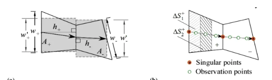
2 2 1 1 1 3 1 sin( ) cos( ) ( ) ( ) 4 j R j r j r m v I e e j H E j u H u H e r u j v v R r r β β β η β β β π β − − − − − − − − − − = − − − + (2.43)If the rooftop footprint is not rectangular, i.e. if it is a trapezoid instead, the field radiated by the basis function is approximated by employing an equivalent width w′, derived from the area A± and height h± of the trapezoid (see Fig. 2.11(a)). Again the employed field expressions describe three spherical waves originating at the top, the bottom and at the centre of the dipole. As a consequence, for calculating the self-term interactions, the observation points can be located directly on the physical surface as in Fig. 2.10(b), avoiding numerical treatment of the singularity.
(a) (b)
Figure 2.10. Geometry and reference system for a bent dipole with different branches lengths H1, H2
2.2.3. Generalized field expressions 43
(a) (b)
Figure 2.11. Scheme for deriving the basis equivalent width (a); singular and observation points for self-term calculation (b).
The generic impedance matrix element is expressed as:
(
, ,)
1 , , , , , 1 1 ( ) ( ) ( ) 1 ( ) ( ) M ij j i i j i i m i m m m S M N i m i m m j n j n i m m n Z E R f dS E R f R S f R S w E R N ± ± ± ± ± = ± ± ± ± ± ± = = = ⋅ = ⋅ ∆ ′ = ∆ ∑
∫∫
∑
∑
(2.44)where N represents the number of radiating dipoles used to calculate the fields Ej n, ± , Ri m, ± is the distance between the source and the M field points, and Sm
±
∆ is an area element (see Fig. 2.11(b)). The field Ej n±, radiated by the basis function is expressed as:
(
) (
ˆ)
ˆj u v u v
E±= E±+E± t++ E±+E± t− (2.45)
where ˆt+and ˆt− represent the directions of +/- test trapezoids respectively. The testing functions fi± are defined by:
2 2 1 1 sin ( ) 0 ( ) sin ( ) 0 m i m I H u H u f u I H u u H β β + ± − + − < < = − < < (2.46)
To avoid charge accumulation at the edges we impose the continuity of the normal component of the current across the common edge (Fig. 2.10(a)) as follows:
1 2 sin sin m m I H I H h h β β − + − = + (2.47)
2.2.4. Numerical solution to the CFIE
As previously shown in section 1.4.2, in the conventional CFIE formulation the EFIE for the field outside the object is combined with the EFIE inside the object to form a combined equation (EFIE-I + EFIE-O). Similarly, the MFIE inside and outside the object are combined in the same way (MFIE-I + MFIE-O).
Let us consider the original problem of EM scattering by an arbitrarily shaped and homogeneous body characterized by (ε2, μ2) (region 2), embedded in an infinite and homogeneous medium having permittivity and permeability ε1 and μ1 respectively (region 1, see Fig. 2.12). The permittivity and permeability can in general be complex to account for losses.
(a) (b) (c)
Figure 2.12. Original scattering problem (a), and equivalent sub-problems in exterior and interior regions R1 (b) and R2 (c) respectively.
The total electric and magnetic fields in R2 are denoted by (E H2, 2)
while in R1 we have 1 1
(E H , ). The normal vector nˆi points into region Ri and S denotes the boundary surface
between R1 and R2.
By applying the equivalence principle, we can derive two equivalent sub-problems to describe the original one: the first sub-problem, equivalent to the original one in region 1 (Fig. 2.12(b)) and the second sub-problem equivalent to the original problem in region 2 (Fig. 2.12(c)). In the null field regions the constitutive parameters are the same as in the non-null field regions, so the equivalent currents ( ,J M i i) radiate into an unbounded homogeneous medium.
The two sub-problems can be related to each other by enforcing the boundary conditions on the tangential components of the electric and magnetic fields, that must be continuous across S. Since nˆ2= −nˆ1 on S, this implies:
2 1 2 1 S S S S J J J M M M = − = = − = (2.48)
For each equivalent representation, the scattered fields produced by the equivalent electric and magnetic currents can be expressed in mixed-potential form as in (1.58), (1.59).
2.2.4. Numerical solution to the CFIE 45
By following this formulation the fields can be directly obtained in closed-form; in particular, the electric and magnetic fields produced by J equivalent in region 1 read:
(
)
(
)
1 2 (1) 1 1 1 2 (1) 1 1 1 1 2(1) 1 2(1) 2 3 2(1) 1 1 2(1) 2 2 1 2(1) 1 2(1) 3 1 2(1) 1 1 1 cos( ) sin( ) 4 sin( ) cos( ) ( ) ( ) 4 i j R j r j r m u j R j r j r m v e e E j I H ju H e R r r j r j H j I e e E u H u H e r u j v v R r β β β β β β η β β π β β η β β π β ± ± ± − − − ± − − ± − ± ± ± ± ± = − − ± + = ± − ± + 1 2 (1) 1 1 2(1) 1 2(1) cos( ) sin( ) 4 j R j r m p j I u H e e H j H v r β β β β π ± ± ± − − ± = − (2.49)where +/- represents the radiating half trapezoid with half length H2(1). The fields scattered by
J equivalent in region 2:
(
)
(
)
2 2 (1) 2 2 2 2 (1) 2 2 2 2 2(1) 2 2(1) 2 3 2(1) 2 2 2(1) 2 2 2 2(1) 2 2(1) 3 2 2(1) 2 1 1 cos( ) sin( ) 4 sin( ) cos( ) ( ) ( ) 4 j R j r j r m u j R j r j r m v e e E j I H ju H e R r r j r j H j I e e E u H u H e r u j v v R r β β β β β β η β β π β β η β β π β ± ± ± − − − ± − − ± − ± ± ± ± ± = − ± + = − ± − ± + 2 2 (1) 2 2 2(1) 2 2(1) cos( ) sin( ) 4 j R j r m p j I u H e e H j H v r β β β β π ± ± ± − − ± = − − (2.50)In order to derive the EM fields radiated by mathematical magnetic currents, the duality relationships: J M E H H E ε µ µ ε → → → − → → (2.51)
are applied to the previous equations and it is obtained, for the fields produced by equivalent M in region 1:
(
)
(
)
1 2 (1) 1 1 2 (1) 1 1 1 2(1) 1 2(1) 2 3 1 2(1) 1 1 2(1) 2 2 2(1) 1 2(1) 3 1 1 2(1) 1 1 1 cos( ) sin( ) 4 sin( ) cos( ) ( ) ( ) 4 i j R j r j r m u j R j r j r m v I e e H j H ju H e R r r j r j H j I e e H u H u H e r u j v v R r E β β β β β β β β πη β β β β πη β ± ± ± − − − ± − ± − − ± ± ± ± ± = − − ± + = ± − ± + 1 2 (1) 1 1 2(1) 1 2(1) cos( ) sin( ) 4 j R j r m p j I u e e H j H v r β β β β π ± ± ± − − ± = − − (2.52)and the fields scattered in region 2:
(
)
(
)
2 2 (1) 2 2 2 (1) 2 2 2 2(1) 2 2(1) 2 3 2 2(1) 2 2 2(1) 2 2 2(1) 2 2(1) 3 2 2 2(1) 2 1 1 cos( ) sin( ) 4 sin( ) cos( ) ( ) ( ) 4 i j R j r j r m u j R j r j r m v I e e H j H ju H e R r r j r j H j I e e H u H u H e r u j v v R r E β β β β β β β β πη β β β β πη β ± ± ± − − − ± − ± − − ± ± ± ± ± = − ± + = − ± − ± + 2 2 (1) 2 2 2(1) 2 2(1) cos( ) sin( ) 4 j R j r m p j I u e e H j H v r β β β β π ± ± ± − − ± = − (2.53)By applying the equivalence principle twice, considering once the currents radiating in an unbounded homogeneous medium with dielectric characteristics ε1, μ1 and then radiating in an homogeneous medium with ε2, μ2; enforcing the continuity of the tangential components of electric and magnetic fields across S it is obtained:
{
}
{
}
2 1 2 1 2 1 2 1 2 1 2 1 tan tan 2 1 2 1 tan tan ( ) ( ) ( ) ( ) ( ) ( ) ( ) ( ) i s s s s i s s s s E E J E J E M E M H H J H J H M H M = − + − = − + − (2.54)and the following matrix equation is derived:
[ ]
[ ]
( ) ( ) ( ) ( ) JJ JM inc E II I E II I i MJ MM inc H II I H II I i Z C E D Y H α β − − − − = (2.55)where the sub-block element of ( ) JJ E II I Z − is defined as: 2 1 , , , , , ( ) 2 , ( ) 1 1 1 1 ( ) ( ) ( ) M N JJ i j i m i m m j n j n R j n R m n Z f R S w E J E J N ± ± ± ± ± ± = = ′ = ∆ −
∑
∑
(2.56) with Ej n R, ( 2)(J2) ± defined in (2.50) and Ej n R, (1)( )J1 ± in (2.49).2.3.1. 3λ square conducting plate 47
2.3. Numerical results
The proposed method uses a type of basis function whose radiated field is expressible in a convenient closed-form. This circumvents the need to use the Green’s function to formulate the problem and having to deal with the singularities of the same. As a consequence, a time advantage in the impedance matrix fill-time is achieved by avoiding the repeated numerical treatment of the integrals involving the Green’s function.
Furthermore, since the formulation deals with the electric fields generated by the basis functions directly, as opposed to vector and scalar potentials typically employed in the conventional MoM formulation, the so called ‘low frequency’ problem, which plagues the latter owing to the presence of the 1/ω factor in the scalar potential term, is no longer a concern in the presented technique, and it is possible to use a uniform formulation for the entire frequency range without having to resort to special basis functions, e.g. the loop-stars. Therefore, the impedance matrix does not suffer from frequency scaling and can be efficiently inverted in the low frequency regime.
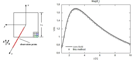
2.3.1. 3
λ square conducting plate
Numerical results for the fields scattered by a flat conducting plate, 3λ on the side under normal plane wave illumination are presented in Figs. 2.13 and 2.14. The magnitude and phase variations of the scattered dominant component are computed varying z from λ to 10 λ.
Figure 2.13. Magnitude variation of scattered Ex computed varying z from λ to 10 λ is compared
Figure 2.14. Phase variation of scattered Ex computed varying z from λ to 10 λ is compared against
conventional MoM result.
Numerical results for the bistatic Radar Cross Section (RCS) for the same test example under normal plane wave illumination are presented on the elevation (Fig. 2.15) and azimuth (Fig. 2.16) planes.
Figure 2.15. Bistatic RCS on the elevation plane for normally incident plane wave on a 3λ square conducting plate.
2.3.1. 3λ square conducting plate 49
Figure 2.16. Bistatic RCS on the azimuth plane for normally incident plane wave on a 3λ square conducting plate.
The results obtained by the present approach agree well with those computed by using the conventional MoM formulation both in the near- and far-field regions.
The time performance in filling the impedance matrix by using conventional techniques and the present approach is reported in Fig. 2.17 as a function of the number of unknowns. The same average edge length of λ/10 is used in the conventional MoM and the proposed method while the number of unknowns is progressively increased.
(a) (b)
Figure 2.17. Comparison of impedance matrix fill-time by using the proposed method and conventional MoM as a function of the number of unknowns (a) and % relative time (b).
The percentage relative time, defined as (Tthis method/Tconv MoM)*100 is plotted in Fig. 2.17(b). It is apparent from the graph that the time advantage in filling the impedance matrix grows as a function of the number of unknowns.
2.3.2. λ conducting cube
The second test example comprises a λ on the side conducting cube on which a plane wave which propagates along -z with E polarized along x is incident. For this example the accuracy is tested by increasing the number of dipoles used to compute the fields radiated by the basis functions. In particular, an augmented number of radiating dipoles as well as testing points is employed to calculate the matrix elements when the separation distance between the basis and testing functions is below the threshold value of 0.2 λ (Fig. 2.18(b)).
(b)
(a) (c)
Figure 2.18. Distance r between source and test basis functions (a); number of dipoles and testing points used when the distance is below (b) or above (c) the threshold value.
Figure 2.19. Bistatic RCS on the azimuth plane for a λ on the side conducting cube. The dipoles used to calculate the fields below the threshold distance are increased from 1 to 3.
2.3.3. λ/2 conducting cylinder 51
Figure 2.20. Bistatic RCS on the elevation plane for a λ on the side conducting cube. The dipoles used to calculate the fields when distance between the basis functions is below the threshold are increased from 1 to 3.
The results obtained by employing one dipole and two testing points per basis everywhere are compared with those obtained by employing three dipoles and six test points per basis when | |r < 0.2 λ. It can be noted that the accuracy is enhanced by using an increased number
of dipoles for the near field interactions.
2.3.3. λ/2 conducting cylinder
In this test example a λ/2 in height and diameter conducting cylinder is analyzed. In Figs. 2.21 and 2.22, we first consider a plane wave incident along the z-direction with the E-field polarized along x and then change the polarization to z and the direction of propagation to x. The bistatic RCS on the elevation plane (φ=0 cut) for the two incident directions is computed and compared against conventional MoM formulation.
The accuracy is tested by increasing the number of radiating dipoles employed to generate the impedance matrix elements associated with the near-field interactions from 1 to 3 (distance between source and test bases | |r < 0.2 λ). As can be noted from Figs. 2.21 and
2.22 an excellent correspondence is achieved against conventional MoM formulation while the accuracy is increased by employing 3 radiating dipoles.
Figure 2.21. Bistatic RCS on the elevation plane for a λ/2 conducting cylinder. The dipoles used to calculate the fields are increased from 1 to 3. The incident electric field is z-polarized.
Figure 2.22. Bistatic RCS on the elevation plane for a λ/2 conducting cylinder. The dipoles used to calculate the fields are increased from 1 to 3. The incident electric field is x-polarized.
2.3.4. 90° corner reflector 53
2.3.4. 90° corner reflector
In the following example we consider a 90° aperture corner reflector λ in length. A plane wave at the frequency of 1 GHz impinges on the structure from θ = 45°, φ = 0°.The bistatic RCS on the elevation plane, φ = 0° (Fig. 2.23) and φ = 90° (Fig. 2.24) cuts is compared against conventional MoM. The accuracy is tested by increasing the number of radiating dipoles employed to generate the impedance matrix elements associated with the near-field interactions from 1 to 3 (distance between source and test bases | |r < 0.2 λ).
Figure 2.23. Bistatic RCS on the elevation plane (φ=0°cut) for a λ conducting corner reflector at oblique incidence. The dipoles used to calculate the fields are increased from 1 to 3.
Figure 2.24. Bistatic RCS on the elevation plane (φ=90°cut) for a λ conducting corner reflector at oblique incidence. The dipoles used to calculate the fields are increased from 1 to 3.
2.3.5. λ/4 dielectric cube
In the next example we consider a λ/4 on the side dielectric cube (εr = 4). A plane wave at the operating frequency of 5 GHz is incident on the structure from θ = 0°, φ = 0°.The bistatic RCS on the elevation (Fig. 2.25) and azimuth (Fig. 2.26) planes is reported below. The scattered electric and magnetic fields and the boundary conditions on the surface of the structure have been formulated as in section 2.3.4.
Figure 2.25. Bistatic RCS on the elevation plane (φ = 0°cut) for a λ/4 dielectric cube at normal incidence.
2.3.6. Low frequency performance 55
2.3.6. Low-frequency performance
A system of equations is defined ill-conditioned when a small change in the system coefficient matrix or a small change in the right hand side results in a large change in the solution vector. The condition number of a system can be measured as the ratio between the relative change in the norm of the solution vector and the relative change in the norm of the right hand side vector. For the system of equations:
x c
Α = (2.57)
the row sum norm of matrix A is defined as:
max 1 1 n i m ij j a < < ∞ = Α =
∑
(2.58)that is, the maximum among the sum of the absolute value of each row of matrix A. By performing a small change in the right hand side vector c of (2.56) a new system of equations is obtained:
x′ c′
Α = (2.59)
Being ∆ = − the change in the right hand side vector, the ratio between the relative c c′ c
change in the norm of the solution vector and the relative change in the norm of the right hand side vector can be expressed as:
x x c c ∞ ∞ ∞ ∞ ∆ ∆ (2.60)
Since it can be shown that:
1 x c x x c − ∆ ∆ ≤ Α Α + ∆ (2.61) and: 1 x x − ∆ ∆Α ≤ Α Α Α (2.62)
are valid, then it is true that the relative change in the norm of the right hand side vector or the coefficient matrix can be amplified by as much as 1
( )
κ Α = Α Α−
, that is called the
This parameter gauges the transfer of error from the matrix A and the vector c to the solution
x. The rule of thumb is that, if κ Α =( ) 10k, then one can expect to lose at least k digits of precision in solving system (2.57) [58].
To demonstrate the applicability of the proposed method over a wide frequency band in a seamless manner we consider the canonical problem of plane wave scattering by a conducting plate whose side is 30 cm and by a conducting sphere whose radius is 15 cm. In the first example a square PEC plate which is λ on the side at the operating frequency of 1 GHz is considered to be invested by a normally incident plane wave with same frequency. The frequency of the incident field is then progressively lowered from 1 GHz down to 1 kHz to reduce the electrical dimensions of the structure.
What we expect is a progressive deterioration of the condition number of the MoM matrix due to a frequency scaling introduced among vector and scalar potentials in calculating the matrix elements as ω→0. The condition number of the matrices computed through the conventional MoM formulation and the presented technique are compared in Fig. 2.27 as a function of frequency.
Figure 2.27. Comparison of impedance matrix condition numbers for the conventional MoM and the proposed method as a function of frequency.
As may be seen from Fig. 2.27, the matrix built by using conventional MoM technique begins to become ill-conditioned from 1 MHz, therefore from 1 MHz down to 1 kHz the conventional MoM solution cannot be trusted.
To demonstrate the reliability of the solution obtained by using our technique compared to that derived through conventional formulations, the canonical problem of scattering from a conducting sphere for which an analytical solution is available, has been analyzed. The matrices condition number obtained through the two formulations have been compared in Fig. 2.28 as a function of frequency.
2.3.6. Low frequency performance 57
Figure 2.28. Comparison of impedance matrix condition number derived through the conventional MoM formulation and the proposed method as a function of frequency.
Again the matrix derived through conventional techniques begins to show an ill-conditioned behavior from 1 MHz. To verify the accuracy of the proposed technique over a wide frequency band, the bistatic RCS on the elevation plane derived through the Mie series, our code and conventional MoM have been compared at some sample frequencies.
In particular, two groups of frequencies have been analyzed; the first group for which the related conventional MoM matrix results well-conditioned (Fig. 2.29) and the other one for which the matrix is ill-conditioned (Fig. 2.30).
Note that while the results obtained from the present approach agree well with those computed by using the Mie series for all frequencies (see Figs. 2.29, 2.30), the MoM solution begins to be inaccurate at 1 MHz (sphere diameter = λ/1000), as may be seen from Fig. 2.30(a), when its impedance matrix begins to become ill-conditioned (Fig. 2.28).
We have introduced a technique for efficient evaluation of MoM matrix elements which leads to well conditioned matrices and also shown that its range of applicability spans over a wide bandwidth covering low frequencies as well.
58 Chapter 2
(a) (b)
(c)
Figure 2.29. Bistatic RCS (elevation) for a R=15cm PEC sphere at 1GHz (a), 750MHz (b) and 250MHz (c).
(a) (b)
Figure 2.30. Bistatic RCS (Elevation) for a R = 15cm conducting sphere at 1MHz (a) and 1 kHz (b). The Mie series, conventional MoM and the results derived through the proposed method are compared.