Università degli Studi di Salerno
Facoltà di Scienze Matematiche Fisiche e Naturali
IN SILICO STUDY OF
PROTEIN-PROTEIN
INTERACTIONS
Philosophiae Doctor Thesis
in
Scienza e Tecnologie dell’Industria Chimica,
Alimentare e Farmaceutica – Indirizzo Chimico
Ciclo XI
Supervisor Contro-relatori
Prof. Luigi Cavallo Prof. Gianluca Sbardella
Prof. Daniele Sblattero
(Università Piemonte Orientale)
Co-supervisor Coordinatore
Dr. Romina Oliva Prof. Gaetano Guerra
(Università Parthenope)
PhD candidate
Anna Vangone
2009-2012
INDEX
ABSTRACT ... 8
CHAPTER 1 - Protein-protein interactions and molecular docking ... 10
1.1 - Introduction to the protein-protein interaction ... 10
Biological complexes: preliminary remarks ... 10
Structure of protein complexes ... 13
1.2 - Approaches to the docking problem ... 15
Step 1: sampling the conformational space ... 17
Step2: scoring and ranking docking decoys ... 18
Biological information ... 20
1.3 - The CAPRI experiment: what is the state of protein-protein docking ... 21
1.4 - The PhD project ... 24
CHAPTER 2 - COCOMAPS: a web tool for analyzing, visualizing and comparing the interface in protein-protein and protein-nucleic acid complexes 25 2.1 - Introduction ... 25
2.2 - Methods ... 26
2.3 - Results and Discussion ... 26
Description of the tool ... 26
The example ... 29
CHAPTER 3 - CONS-COCOMAPS: a novel web tool to measure and visualize
the conservation of inter-residue contact in multiple docking solutions ... 32
3.1 - Introduction ... 32
3.2 - Methods ... 34
3.3. CAPRI models ... 36
3.4 - Results and Discussion ... 37
Inter-residue conservation versus L_rmsd ... 37
Conservation and Consensus maps for the multiple solutions submitted by each predictor ... 38
Consensus maps for the multiple solutions submitted by all the predictors ... 41
3.5 - Conclusions ... 47
CHAPTER 4 - CONS-RANK: a novel tool to rank multiple docking solutions based on the conservation of inter-residue contacts ... 49
4.1 - Introduction ... 49
4.2 - Methods ... 51
RosettaDock benchmark ... 52
DOCKGROUND benchmark ... 52
CAPRI models ... 52
4.3 - Results and Discussion ... 53
Ranking of decoys in the Global-Unbound RosettaDock benchmark ... 54
Ranking of decoys in the DOCKGROUND benchmark ... 58
Ranking of CAPRI targets ... 61
Dependence of the method performance on the percentage of native-like solutions ... 63
Analysis of merged decoys from RosettaDock and DOCKGROUND ... 64
4. Conclusions ... 66
CHAPTER 5 - Study of the interaction between celiac auto-antibodies and the auto-antigen Tissue Transglutaminase (TG2) ... 76
5.1 - Introduction ... 76
The immune system ... 76
The autoimmunity and celiac disease ... 78
Experimental studies ... 80
5.2 - Methods ... 82
Abs and TG2 strucutres ... 82
Docking simulations ... 82
Analysis... 82
5.3 - Results and Discussion ... 82
Abs/TG2 open systems ... 87
Abs/TG2 closed systems ... 87
Finding the key-residues for the interaction ... 87
Simulations on the mutants ... 90
5.4 - Conclusion ... 93
CHAPTER 6 - Prediction and analysis of an idiotype - anti-idiotype antibody complex associated to celiac disease ... 94
6.1 - Introduction ... 94
The idiotypic network ... 94
Anti-idiotypic antibody for cancer immunotherapy ... 97
The role of the anti-idiotypic antibodies in autoimmune diseases ... 98
6.2 - Methods ... 101
Abs modeling ... 101
Docking ... 101
Analysis... 101
6.3 - Results and Discussion ... 102
‘Blind docking’ ... 102
6.4 - Study of experimental cases from literature: comparison with other Ab1-Ab2 X-ray structures ... 106
6.5 - Searching for structural similarities between Ab2 and Ag ... 108
6.6 - Conclusion ... 109
CHAPTER 7 - Dynamic properties of a pathogenic mutant of the blood coagulation Factor X activated (FXa) and their effect on the substrate recognition and the catalytic efficiency ... 110
7.1 - Introduction ... 110
Factor X ... 110
7.2 - Methods ... 113
Molecular dynamics simulations and electrostatic potential calculations ... 113
7.3 - Results ... 115
RMSD and RMSF analysis ... 115
Catalytic hydrogen bonds ... 118
Essential dynamics ... 120
7.4 - Discussion ... 122
7.5 - Conclusion ... 125
APPENDIX 1 - Differences between membrane and soluble protein loop structures ... 126
Introduction ... 126
Methods ... 128
Test set ... 128
Loop angle θ ... 128
Contact number Ncontact ... 129
Results and Discussion ... 130
Conclusion ... 133
APPENDIX 2 - Docking technique: details ... 134
Docking tecnique ... 134
Docking steps ... 134
Fast Fourier Transform ... 136
Monte Carlo method ... 136
Scoring and ranking docking decoys ... 137
The flexibility problem ... 138
Critical Assessment of Prediction of Interactions (CAPRI) ... 139
Docking programs ... 141
RosettaDock ... 141
ZDOCK ... 141
ClusPro ... 143
Conclusive notes ... 143
CONCLUSIONS ... 144
REFERENCES ... 147
LIST OF PUBBLICATIONS AND CONFERENCES ... 162
ABSTRACT
Protein-protein interactions are at the basis of many of the most important molecular processes in the cell, which explains the constantly growing interest within the scientific community for the structural characterization of protein complexes.1 However, experimental knowledge of the 3D structure of the great majority of such complexes is missing, and this spurred their accurate prediction through molecular docking simulations, one of the major challenges in the field of structural computational biology and bioinformatics.2,3
My PhD work aims to contribute to the field, by providing novel computational instruments and giving useful insight on specific case studies in the field. In particular, in the first part of my PhD thesis, I present novel methods I developed: i) for analysing and comparing the 3D structure of protein complexes, to immediately extract useful information on the interaction based on a contact map visualization (COCOMAPS4 web tool, Chapter 2), and ii) for analysing a set of multiple docking solutions, to single out the key inter-residue contacts and to distinguish native-like solutions from the incorrect ones (CONS-COCOMAPS5 web tool and CONS-RANK program, Chapter 3 and 4, respectively).
In the second part of the thesis, these methods have been applied, in combination with classical state-of-art computational biology techniques, to predict and analyse the binding mode in real biological systems, related to particular diseases. This part of the work has been afforded in collaboration with experimental groups, to take advantage of specific biological information on the systems under study. In particular, the interaction between proteins involved in the autoimmune response in celiac disease6,7 (Chapters 5 and 6) has been studied in collaboration with the group directed by Prof. Sblattero, University of Piemonte Orientale (Italy) and the group directed by Prof. Esposito, University of Salerno (Italy). In addition, recognition properties of the FXa enzymatic system8 has been studied through dynamic characterization of a FXa pathogenic mutant that causes problems in the blood coagulation cascade (Chapter 7). This study has been performed in collaboration with the group directed by Prof. De Cristofaro, Catholic University School of Medicine, Rome (Italy) and the group
directed by Prof. Peyvandi, Ospedale Maggiore Policlinico and Università degli Studi di Milano (Italy).
Finally, during my PhD I spent seven months in the groups of Prof. Charlotte Deane, Department of Statistics, University of Oxford (UK). During this period I studied the geometrical features of the proteins’ regions most recurrent in the protein-protein interaction, the loops, clarifying some structural aspects of them in one of the most important and huge class of proteins: the membrane proteins (Appendix 1).
Web tools and programs:
COCOMAPS4 web tool freely available at:
https://www.molnac.unisa.it/BioTools/cocomaps/
CONS-COCOMAPS5 web tool freely available at:
https://www.molnac.unisa.it/BioTools/conscocomaps/
CHAPTER 1 - Protein-protein interactions and molecular
docking
1.1 - Introduction to the protein-protein interaction
Biological complexes: preliminary remarks
The thousands of proteins expressed in the cells perform many of their functions through interactions with other proteins. The protein-protein interactions are intrinsic to every cellular process; in fact, protein complexes have been implicated as an essential component in the major research topics in biology and medicine, such as DNA replication, transcription, translation, splicing, secretion, cell cycle control, signal transduction, and intermediary metabolism.1,9 Therefore, the analysis at a molecular level of proteins in complexes is a matter of interest for biochemists, but also geneticists, cell biologists, developmental biologists, molecular biologists and biophysicists.10
Protein-protein interactions play diverse roles and differ based on the composition, affinity, lifetime and nature of the association. In the permanent/obligate complexes the interactions are usually very stable and the interacting proteins are not found as stable structures on their own in vivo, while in the transient/non-obligate complexes there are transient interactions that associate and dissociate in vivo and the interacting proteins can also exist in the unbound form. Obligate complexes can be further divided into homodimers, i.e. interactions occurring between identical chains, heterodimers and multimers.11 It has been observed that different classes of association exhibit different physical and chemical properties in their interaction sites and different functions.12-14 So, for example, interactions in intracellular signaling are expected to be transient, since their function requires a ready association and dissociation, while an antigen-antibody interaction is generally permanent. Anyway, it is important to note that many protein-protein interactions do not fall into distinct types. Rather, a continuum exists between non-obligate and obligate interactions, and the stability of all complexes very much depends on the physiological conditions and the environment.11
principles of protein-protein interactions.15-20
The formation of biological complexes is driven by the free energy of the complex (determined by physicochemical and geometrical interface properties) and the concentration of the protein components.11 The association of two proteins, in fact, relies on an encounter of the interacting surfaces, requiring co-localization in time and space. Generally a protein resides in a crowded environment with many potential binding partners with different surface properties; therefore, during the evolution the surfaces presumably evolve to optimize the interacting efficacy.21 When proteins
collide, they do not diffuse away immediately (kinetic experimental evidence from Northup et al.22 and Wells23); instead, they are held loosely, rolling on one another
and thereby sampling considerably more surface area than would be the case for a single elastic collision; this allows them time to become reorientated and repositionated on the surface or to adjust their shape to fit together more tightly (Figure 1).24 Recent studies are beginning to describe the dynamic of the assembly processes and to show that these non specific collisions producing transient ‘encounter complexes’ play an important role in macromolecular associaction.25 The role of long-range forces in bringing molecules together has been studied from both experimental and theoretical viewpoints,26,27 suggesting the electrostatic interactions to be predominant.25
Figure 1. Protein-protein interactions
Equilibrium steps in a possible mechanism for protein–protein association. a) Formation of transient encounter complexes by nonspecific collisions, guided mostly by electrostatic interactions. b) Many encounter complexes separate rapidly. c) Some productive encounter complexes reorientate and come closer to the final, specific orientation, guided mostly by desolvation, as water molecules move away from the protein surfaces. d) Formation of the specific complex, with final fitting of interacting surfaces.24
In this scenario, it is extremely valuable to obtain structural information for a complete understanding of both the biochemical nature of the process for which the components come together, and the facilitated design of compounds that might influence it. In particular, the structural characterization of a protein-protein interface includes the identification of interatomic hydrogen bonds, of salt bridges, of hydrophobic interactions, determination to the interaction surface area and possibly the presence of bridging water molecules28,29 The combination of all this information about the network of interactions defines the nature of the binding site and makes it possible to point out the residue-residue contacts with a key role in the interaction. Here below it is reported an example of a protein-protein interface characterization for the complex between the hemagglutinin (HA) and its antibody HC45.30 This antigen-antibody complex has a fundamental role in one of the most common world diseases: the influenza. Hemagglutinin, in fact, is the influenza virus glycoprotein that interacts with infectivity-neutralizing antibodies. It has a primary role in influenza infection mediating the binding of the virus to its cellular receptor. Over the years, amino acids substitution that arise by mutations in the genes for HA lead to escape of immune surveillance and recurrent epidemics - this process is called antigenic drift. So, the structural study of the complexes between HA and its antibodies is fundamental to understand the mechanism of the infection and to ensure the development vaccines of variants closely related to the circulating virus. Fleury at
al.30 reported the structure of the X31 HA-HC45 Fab complex (PDB entry: 1QFU; resolution 2.8 Å), describing the atomic characteristics of their interactions (Figure 2). Upon complex formation, a surface area of 1.840 Å2 is buried; 36 amino acids participate in the intermolecular contacts, and 10 hydrogen bonds are established, involving antigen’s residues such as Asp36 and Arg94. The HC45 epitope, i.e. the antigen binding site, comprises in total 17 residues. It was also proved that the mutation Asp63Asn (Figure 2, right) leads to escape from neutralization by HC45, underlining the importance of this residue in the interaction.
Figure 2
The X31 HA–HC45 Fab complex. Left: Ribbon diagram of the complex showing one HA monomer (the two domains HA1 and HA2 in blue and res, respectively) and the HC45 Fab (in green); the receptor binding site is shown in yellow. Right: Stick view of the HC45–HA interface (HA in blue, Fab in green). Of the 17 amino acids in the epitope, 12 are in the four polypeptide stretches of the HA1 chain (residues 59–63, 78–79, 90–94 and 271–273) and are represented here. HA residues substituted in mutants with decreased affinity for the HC45 antibody (Asp63 and Arg94) are highlighted in cyan; their nitrogen and oxygen atoms are colored in cyan and red, respectively. Hydrogen bonds involving atoms of these HA residues are shown as dotted lines.30
Structure of protein complexes
As shown in the example, the structural characterization of biological complexes has a supreme significance in the study of the system and in all the possible pharmaceutical and medicinal applications,31 and although experimental methods for protein-structure determination have improved over the past decade, the number of structures for protein complex determined is still very little. Protein structures have been mainly achieved by two methods so far: X-ray crystallography and nuclear magnetic resonance (NMR). X-ray and NMR encounter difficulties to prepare complexes suitable for structural studies: by X-ray, the dynamics of the complex formation makes the crystallization difficult, while complexes of high molecular weight are difficult to deal with NMR.18,32,33
Due to the greater difficulty in obtaining suitable protein-protein complexes for the experimental determination, there is relatively little structural information available
about them compared to the proteins that exist as single chains or form permanent oligomers.33 Hence, experimental studies are faced with outstanding technical difficulties and the number of solved complexes deposited in the Protein Data Bank34 (PDB: www.rcsb.org/pdb) is still orders of magnitude smaller than structures of individual proteins, as show in Figure 3.18,31
Figure 3
Number of X-ray structures of protein-protein complexes (in green) and single chain proteins (in blues) deposited in the wwPDB34 within October 2011.
Despite this disproportion, the growing number of available experimental structures for protein-protein complexes in the years has allowed a statistical study of the properties and the chemical-physical forces that regulate protein-protein interactions (hydrophobicity, hydrogen bonding, electrostatic interactions, van der Waals interactions, and so on), that are useful information in the development of computational strategies helping in the structural prediction and characterization.35 In
fact, notwithstanding the practical difficulties, for a better understanding of the biological function of a protein, knowledge of its three-dimensional structure is fundamental. Therefore, it would be quite rewarding to have efficient and reliable computational algorithms available to predict correctly conformations of protein complexes based on the structures of the free molecules. Indeed, in the past two decades there was an emergence of a large variety of theoretical algorithms designed to predict the structures of protein-protein and protein-ligand complexes: a procedure
named molecular docking.36
Interest in protein docking is growing within the scientific community, and many interdisciplinary approaches are being applied to model, predict, and understand protein-protein interactions, one of the major challenge in the field of structural bioinformatics. 37
1.2 - Approaches to the docking problem
The docking technique has the task of assembling two separate protein components (as the ones seen in Figure 4a and Figure 4b) into their biologically relevant complex structure (Figure 4c), giving a model of the way the two proteins bind each other.38,39 Computational docking, if accurate and reliable, can therefore play an important role, both to infer functional properties and to guide new experiments. So, due to its potential applications in generating models of molecular complexes, it has attracted a vast deal of attention.40
Figure 4. Schematic representation of the protein-protein docking technique X-ray structure of (a) FAB Hyhel63 antibody (PDBID: 1DQQ), (b) HEW lysozyme (PDBID: 3LZT) and (c) the biological complex formed between the two (PDBID: 1DQJ).
The docking in general, and the protein-protein docking in particular, is not a simple problem. The objective of it is to predict the three-dimensional arrangement of a protein-protein complex from the coordinates of its component molecules, hopefully pointing out most of the residue-residue contacts involved in the interaction.41-47 There are no general rules to predict a binding interface. Basically, all docking approaches assume that the native complex is near the global minimum of the energy landscape. In fact, based on thermodynamic hypothesis, at fixed temperature and pressure the Gibbs free energy of the macromolecule-solvent system reaches its global minimum at the native state of the complex.48 It has been established over the
last two decades that the energy landscape of a foldable protein resembles a many-dimensional funnel with a free energy gradient toward the native structure (Figure 5).21,49,50 A number of studies suggest that the landscape theory also applies to protein-protein association.51-54 This theory states that the assembly of two proteins is initiated by the formation of nonspecific encounter complexes,24 followed by rearrangements of them driven by stronger and more specific interactions. Taking into account that it is the structural features that determine if two proteins interact,55 then such hypothesis implies that not only the ‘final’ binding but also other parts of the surface contain information for interacting with the partner. The size of the funnel will be determined by the length scales of the long-range electrostatic and hydrophobic interactions and the geometry of the proteins, and hence the funnel is restricted to a neighborhood of the native complex.56 There is a free energy gradient toward the native state, but the funnel is rough, giving rise to many local minima.21,57
Figure 5. Protein-protein complex energy landscape
The many-dimensional funnel representing the energy landscape of a protein-protein complex. With “N” the native conformation is indicated.
Therefore, all the current docking methods are based on the optimization of a function approximating the free energy of the complex.
In all the docking algorithms, there are two crucial steps to generate possible models of the three-dimensional arrangement of a complex:
1. Searching (low-resolution search), consisting in the generation of thousands of alternative poses (decoys) to sample the rotational/translational space; 2. scoring and ranking (high-resolution refinement), consisting in scoring these
poses using a ‘pseudo-energy’ function in order to rank the poses and so to identify the native-like solutions.
A simple docking algorithm may fail predicting the native complex. Anyway, a recent work58 shows that the docking technique is able to distinguish between binding and non-binding partners, based on their score distributions. This may indicate that although protein surface morphology is not enough to find the native interface, it at least contains sufficient information to identify a ‘bona fide’ interactor.58
Anyway, it has been shown in CAPRI that, whereas approximately correct solutions are generated by the first step of the docking, scoring functions unfortunately often fail to correctly rank them.58,59
Step 1: sampling the conformational space
The searching step involves an exhaustive search of the conformational space of one protein with respect to the other, resulting in a six-dimensional search (6D). The search of through the entire conformational space of the complex geometry makes the calculation expensive, so it is necessary to simplify the system preserving the geometrical and physicochemical properties of the atoms, using mathematical models, such as geometrical shape descriptors or a grid.42 Once having the easier
representation of the system, almost all the docking programs use the same approach for the searching step: one protein is fixed in space (usually the bigger one) and the second one is rotated and translated around the first one. To minimize the degrees of freedom, both molecules are treated as rigid bodies, but still a simple systematic search is usually impracticable because the searching algorithm entails evaluating in
Although geometric complementarity of the protein surface is the filtering criterion most commonly used to eliminate a large number of solutions with poor surface matching,47 the docking problem is not simply matching two irregular shapes, but there are also other geometric, electrostatic or hydrophobic factors to take into account.61
So, there are a lots of possible search methods that have been used in protein-protein docking programs. Most methods that perform well in CAPRI are based only on three approaches. Some programs use grid-based spatial searches that are sped up with a Fast Fourier Transform (FFT), a method first applied in 1992 by Katchalski-Katzir and co-workers.62 The other approaches for docking searches include instead Monte
Carlo based searching63,64 and geometric hashing.65
Step2: scoring and ranking docking decoys
The initial stage, which treats proteins as rigid bodies and generates many prediction (10.000 or more), is followed by the refinement stage, which performs any combination of detailed scoring, energy minimization, side chain optimization to the aim of valuate the energies of protein-protein docking poses in order to identify the one with the lowest energy as the predicted binding mode.47
A fundamental point of any docking method is to be computationally efficient, having a scoring scheme able to evaluate a huge number of solutions and discriminate the native-like binding modes from the wrong decoy complex structures in a reasonable computational time.42
The free energy of binding, ΔGbinding, is not easily accessible but other and faster
scoring functions that model ΔGbinding as accurately as possible, i.e. provide good
correlations with experimental binding affinities, can be used.60 Considering the energy function as a funnel-like function, as described above, the original free energy function is extremely rugged with huge number of local minima even in a small region of conformational space. Yet its approximated scoring function is much smoother and still capture the overall funnel-like landscape, which provides an easier free energy minimization (see Figure 6).66 Further, according to the general idea of the funnel-shaped binding energy, there are an ensemble of encounter complexes from which the binding process initiates and precedes, that follow different pathways to converge in native state defined by the global minimum. So, there are many
possible routes for downhill in the binding funnel, and these are determined by transient interactions in the encounter complexes, which carry a track of the native interactions.24
Figure 6
The schematic representation of a funnel-like function (dark line) and an approximated scoring function (dotted line), still catching some of the local minima (indicated as small squares).
Whether this ensemble of orientations reflects the true binding-energy landscape will depend on the accuracy of the energy description and the efficiency of the sampling method. Most of the docking algorithms developed so far use the extent of geometric complementarity of the protein surfaces because it is a fast filter to eliminate a large number of solutions with poor surface matching. It is, however, usually recognized that a criterion based exclusively on geometric complementarity is far from being enough to distinguish among native and non-native docked geometries, except for a very a small number of cases.67 Numerous criteria have been implemented with
different levels of success: steric complementarity of the shapes of the interaction sites, electrostatic interactions, hydrogen bonding, van der Waals, pair potential, desolvation, rotamer probabilities, contact pair potential and knowledge-based potentials. Different docking programs can use different combinations of these terms in a weighted sum. Furthermore, exclusion of the solvent from the interface and the associated solvent entropy change play an important role in the stabilization of protein interactions, and can be estimated from empirical potentials or database derived functions.18,68
retained and ranked. A common way to rank the retained decoys is clustering them using pairwise root mean square deviation (RMSD, a number that quantifies the structural diversity between two structures) as the distance measure, and then ranks the clusters according to their size, i.e., identifying conformations that have large numbers of neighbors.56,57 The method is based on the observation that, in the free energy landscapes of partially solvated receptor-ligand complexes, the free energy attractor at the binding site generally has the greatest breadth among all local minima.69 Hence, following the uniform sampling of the conformational space
defined by translations and rotations of the ligand, the docked conformations that are below an energy threshold are expected to form the largest cluster around the native complex.
Biological information
Although important progresses, protein-protein docking remains a quite difficult procedure, due to the complex nature of the problem it tries to solve. One of the most useful approach to improve the quality of the docking simulations is the use of biological information about the complex interface to confine the search of allowed configurations or filter out wrong solutions.42,70 Biological information available from experiments or from computational methods on the regions or residues likely involved in the interaction are one of the key points for the improvement of a docking simulation. Almost all the docking programs have a section in which it is possible to exclude regions not involved in the interaction, or driving the docking towards the ones involved (for example, the software HADDOCK32 dedicate a section to express the NMR data such as chemical shift perturbation and residual dipolar couplings in terms of ambiguous interactions restrains). If experimental data are not available for the protein-protein system that is simulated, it is also very helpful to carry out structural comparisons of the same protein family.42,70 Fox example, the binding crevice centered on the catalytic triad of serine proteases (His, Asp, Ser)71,72 (see
Chapter 7), as well as the complementarity defining regions of immunoglobulins (CDRs), which are part of the biological surface involved in the interaction with protein interactors (see Chapter 5 and Chapter 6), are both well characterized; although in general, a protease-inihibitor interface is more static and consequently more easily predicted than an antibody-antigen interface.73
1.3 - The CAPRI experiment: what is the state of protein-protein
docking
As described above, protein-protein docking procedure is a very helpful method to model biological complexes and to guide biochemical experiments. A general docking algorithm can be briefly described as an initial searching step yields a long list of candidate structures; the following step requires some forms of post-processing, which may include: i) scoring or re-scoring of the docked conformations using a more accurate energy function, or ii) refining the conformations followed by re-scoring.74 These treatments usually improve the number of near-native conformations among the 10 to 100 lowest energy structures, but in most cases are unable to eliminate all false positives (steps showed in Figure 7).
Figure 7
The stages of protein-protein docking.
A variety of approaches have been used in docking programs that mostly differ in the stages of the algorithms, showing different performances depending on the approach and the nature of the biological system. In this scenario, the comparison of different
docking programs to establish their relative performances is very important. Indeed, it is required an objective valuation of the model quality. To this aim, the international Critical Assessment of Prediction of Interactions (CAPRI) experiment was designed, precisely to evaluate current computational approaches of protein–protein docking.75 The CAPRI is a community-wide experiment designed according to the model of the Critical Assessment of Techniques for Protein Structure Prediction (CASP).76 It was designed in June 2001 at the Conference on Modeling Protein Interactions in Genomes organized in Charleston, SC, by Ilya Vakser (Medical University of South Carolina) and Sandor Vajda (Boston University). CAPRI targets are protein–protein complexes and it is data-driven, meaning that it can start whenever an experimentalist offers an adequate target and ends 6–8 weeks later with the submission of predicted structures.76-78 Computational researchers are given the three-dimensional coordinates of the unbound structures for a given target before the experimental structure of the complex is published. The researchers are then given a few weeks to dock the two structures together, possibly using biological information and literature searches. Therefore, CAPRI challenge provides the docking community with a unique blind setting of simultaneously assessing of all docking algorithms, and has led to significant advances in the field.79,80
From the analysis of CAPRI results, it can be noted that there are some docking programs that give globally better predictions, such as ICM,81 ZDOCK,79 HADDOCK,32 RosettaDock,64,82 ClusPro56 and Camacho group’s Smooth-Dock.75 Furthermore, in Figure 8, the number of citations per year of the most common docking programs joining to CAPRI is plotted (references took from ISI Web). From the plot it is possible to observe that only after 2003 there was an increase of the number of citations of the protein–protein docking software. Since their publication the most cited programs are HADDOCK,32 RosettaDock,64 three-dimensional-Dock,83 BIGGER,67 and Dot.53 It is possible to observe an increase of the number of citations
per year of the Patch-Dock,44,45 ClusPro,56 HADDOCK,32 RosettaDock64 and
ZDOCK.79 When considering only papers that apply the different software to specific
biological problems (represented in Figure 8b) HADDOCK results to be the most popular one, followed by ClusPro, PatchDock and RosettaDock.
Figure 8
Number of citations per year of the docking programs described earlier. Data taken from ISI Web of Science (February of 2007).; only the articles with experimental predictions were considered.
Four of the most common docking programs are RosettaDock,64 ZDOCK,79 HADDOCK32 and ClusPro.56 The advantage of RosettaDock compared with the other three programs is the close correspondence of the lowest free energy structures with the X-ray complex, the disadvantage is that using a Monte Carlo technique in the searching step and a detailed energy function, it is quite slower than the others. Instead, ZDOCK is a FFT based algorithm, so it is faster but it does not perform well in the cases of complexes with large conformational change. HADDOCK seems combine the rapidity with the fact that the both side chains and backbone are allowed to move, and this increase the accuracy of the scoring if compared with classical rigid body docking programs. The big disadvantage in HADDOCK is that it is data-driven, so its performance closly depends on the availability and the level of confidence of experimental information. Compared with the other programs, ClusPro has the advantage to be a fully automated algorithm that rapidly docks, filters and ranks potential models within a short amount of time, using only the structures of the component proteins, and eventually adding experimental data if available.
1.4 - The PhD project
My PhD work has been focused on the study of protein-protein interactions, taking advantage of computational techniques. The study has been devoted to two main aspects: i) the development of new methods to analyse and rank docking solutions (Chapters 2,3,4), and ii) the application of these methods, in combination with classical state-of-art computational biology simulations, to predict and analyse the binding mode in real biological systems, which are related to particular diseases (Chapters 5,6,7). As availability of biological information is guarantee of a better success rate in the docking simulations, we afforded the latter part of the work in collaboration with experimental groups. In particular, interaction between proteins involved in the autoimmune response in celiac disease has been studied in collaboration with the group directed by Prof. Daniele Sblattero, University of Piemonte Orientale (Italy) and the group directed by Prof. Carla Esposito, University of Salerno (Italy). In addition, recognition properties of the FXa enzymatic system has been studied through dynamic characterization of a FXa pathogenic mutant that causes problem in the process of blood coagulation. This study has been performed in collaboration with the group directed by Prof. Raimondo De Cristofaro, Catholic University School of Medicine, Rome (Italy) and the group directed by Prof. Flora Peyvandi, Ospedale Maggiore Policlinico and Università degli Studi di Milano (Italy). Finally, during my PhD I spent seven months in the groups of the Prof. Charlotte Deane, Department of Statistics, University of Oxford (UK). In that period, I studied the geometrical features of the proteins’ regions most recurrent in the protein-protein interaction, the loops, clarifying some structural aspects of them in one of the most important and huge class of proteins: the membrane proteins (Appendix 1).
CHAPTER 2 - COCOMAPS: a web tool for analyzing,
visualizing and comparing the interface in protein-protein
and protein-nucleic acid complexes
2.1 - Introduction
Interaction between biomolecules is at the basis of many of the most important molecular processes in the cell. As described in Chapter 1, protein-protein interactions underlie for instance signaling, regulation, immunogenic recognition, whereas protein-nucleic acid interactions under- lie processes such as DNA transcription, repair, replication, as well as post-transcriptional events, including RNA splicing and editing.
Availability of a 3D structure for a complex allows detailed analysis of the interaction at atomic level between the molecular partners, which is a fundamental step for possible biomedical and biotechnological applications. Moreover, the recent development of well performing docking software (see Chapter 1 and Appendix 2) to predict the 3D structure of macromolecular complexes requires, in the analysis step, the accurate and tedious screening of all the best solutions. It is indeed well accepted that the correct solution, if any, can be found within the 10-20 best ranked ones (e.g. the CAPRI assessment accepts 10 different models per target from each predictor). It is therefore of timely interest, both for bioinformaticians and wet biologists, to have programs and tools able to automatically analyse features of a complex interface, and to easily and intuitively discriminate between similar and different binding solutions Several valuable web tools have been made available for the analysis of the interface in biomolecular complexes.84-92 However, no available web tool has been implemented to provide interactive contact maps from the 3D structure of a biomolecular complex.
Introduced to provide a reduced representation of a protein structure, contact maps have been successfully exploited for describing similarity between protein structures. Analogously, an intermolecular contact map between two or more interacting molecules could identify uniquely and intuitively the surface of interaction, representing a sort of fingerprint of the complex and reporting the crucial information
in a ready-to-read form. Interesting work has in fact been done to demonstrate the advantages of using contact map representations for the alignment of protein-protein interfaces.93,94
For this reason, during my PhD study my groups and I have implemented COCOMAPS (bioCOmplex Contact MAPS).4 It is a novel web tool to easily and effectively analyse and visualize the interface in biological complexes, such as protein-protein, protein-DNA and protein-RNA complexes, by making use of intermolecular contact maps.
2.2 - Methods
All the programs under COCOMAPS have been written in python, taking advantage of python libraries such as SciPy and Matplotlid. We made it available at the URL:
http://www.molnac.unisa.it/BioTools/cocomaps.
2.3 - Results and Discussion
Description of the tool
The tool takes in input the PDB type file of the complex, that contains the Cartesian coordinates of the complex. Usually, the two interacting parts of the complex are distinguished by different names of the chains, indicate by a single letter. In fact, a user-friendly interface of the tool allows to download input files directly from the data bank wwPDB95 (for the experimental structures) or to upload locally stored PDB
formatted files. The user is requested to specify the chain identifiers for the molecules involved in the interaction to be analyzed. More chains can be selected for each interacting partner, which overcomes a limitation of the other available tools that either work on all the chains present in a PDB file, or on one pair of them at a time. Therefore, COCOMAPS can be used to analyze the interface between two molecules, between one molecule and an ensemble (made by two or more molecular chains) or between two ensemble, depending on how many chains are specified.
COCOMAPS outputs are displayed on the results HTML page for one month and archived as downloadable compressed files. A link to the online resource is also emailed to the user, if requested.
COCOMAPS provides three graphical contact maps defining the interface of the complex:
1. Black and white contact map;
2. Distange range contact map;
3. Properties contact map.
The first one is a classical intermolecular contact map (Figure 9, a) where a black dot is present at the crossover of residues i and j, belonging to molecule/assembly 1 and molecule/assembly 2, respectively, if any pair of atoms belonging to the two residues is closer than a cut-off distance chosen by the user (default value being 8 Å). The second map (Figure 9, b), named “distance range contact map”, reports in different colors inter-residues contacts at increasing distances. Red, yellow, green and blue indicate contacts within 7 Å, 10 Å, 13 Å and 16 Å, respectively. The third contact map (Figure 9, c), named “properties contact map”, is similar to the first one, but each contact is colored according to the physico-chemical nature of the two interacting residues: hydrophobic-hydrophobic in green, hydrophilic-hydrophilic in violet and hydrophobic-hydrophilic in yellow.
By mousing over the maps, it is possible to visualize the identity of the residues pairs corresponding to the dots.
Figure 9.
A sample of COCOMAPS contact maps for the complex Ibalizumab antibody (chains L and H) with the CD4 antigen (chain A), PDBcode: 3O2D. a) Black and
white contact map; b) Distance range contact map; c) Properties contact map.
Our tool also provided detailed information, organized in table (Figure 10, a and b), about:
1) interacting residues, defined on the basis of a cut-off distance that can be customized by the user;
2) residues at the interface, defined on the basis of the buried surface upon complex formation;
3) intermolecular H-bonds, with specification of the acceptor and donor atoms. A 3D visualization of the complex in JMol (http://www.jmol.org) (Figure 10, c) is also provided online, with the interacting residues highlighted. Finally, a ready-to-run Pymol96 script, which generates a visualization of the interface in the corresponding
All the programs under the COCOMAPS web tool have been written in python, taking advantage of python libraries such as SciPy and Matplotlib.
Figure 10.
Sample COCOMAPS outputs for the complex Ibalizumab antibody (chains L and H) with the CD4 antigen (chain A), PDBcode: 3O2D. a) First part of the table of
interacting residues, defined on the basis of the cut-off distance; b) Overview table of
the interaction properties ; c) 3D visualization of the complex in Jmol
The example
Although COCOMAPS provides a complete characterization of the interfaces in biological complexes, the real novelty that we have introduced is the generation of intermolecular contact maps. Contact maps give an immediate view of which regions of the two partners are in contact. From the properties map, it is also possible to immediately appreciate the physico-chemical nature of the interaction.
As an example, in Figure 11 properties contact maps are reported for the biological complexes of the antigen hen egg lysozyme (HEL) with two different antibodies, namely D1.3 (PDBcode: 1VFB)99 and F10.6.6 (PDBcode: 1P2C)100, together with the corresponding Pymol 3D representation of the complexes, as generated by COCOMAPS.
corresponding epitopes present no overlap. In addition, contact maps specify which regions of the antibodies and of the antigen are in contact.
As expected, both the antibodies contact HEL with their six hypervariable loops (L1, L2, L3, H1, H2 and H3, also labeled in the figure, for the sake of clarity). As for the HEL antigen, it contacts the D1.3 antibody with about 30 N- and 30 C-terminal residues and the F10.6.6 antibody with its central region (residues 40-85). The same information could of course be extracted either from lists of interacting residues or from the 3D view of the complexes (such as that in Figure 11). However, differently from the contact-map view, which is immediate, in both of the above cases, manual intervention by the user would be required to extract the needed information. Further, the contact maps in Figure 11 immediately indicate that the H3 loop of the D1.3 antibody is more involved in the interaction with HEL than the F10.6.6 H3 loop, and that it mostly gives hydrophilic-hydrophilic contacts (magenta dots). This is a consequence of the D1.3 H3 loop amino-acids sequence, (one code amino-acids sequence: ERDYRLDY), which is longer than the F10.6.6 one (one code amino-acids sequence: GDGFYVY), and much more hydrophilic, presenting five charged residues.
Figure 11.
Comparison of the complexes of HEL with two different antibodies: D1.3 (PDBcode: 1VFB) and F10.6.6 (PDBcode: 1P2C). Left: COCOMAPS “properties contact maps”. Labels have been added for the antibody hypervariable loops L1-L3 and H1-H3. Magenta, green and yellow dots indicate hydrophilic-hydrophilic, hydrophobic-hydrophobic and hydrophobic-hydrophobic-hydrophilic contacts, respectively. The cut-off distance is set to 10 Ǻ. Right: A Pymol visualization of the complexes based on the automatic COCOMAPS script .pml; residues at the interface are shown as "sticks".
2.4 - Conclusion
In conclusion, this first study has been focused on the development of a tools able to automatically analyze, visualize and compare the interfaces both in experimental and predicted 3D structures of protein-protein and protein-nucleic acids complexes. COCOMAPS combines in a single tool the traditional analysis and 3D visualization of interfaces in biocomplexes with the effectiveness of the contact map view. It can straightforwardly be applied to the analysis of interfaces both in experimental and predicted 3D structures of biological complexes.
CHAPTER 3 - CONS-COCOMAPS: a novel web tool to
measure and visualize the conservation of inter-residue
contact in multiple docking solutions
3.1 - Introduction
As described in Chapter 1, most important molecular processes in the cell rely on the interaction between biomolecules. Understanding the molecular basis of the recognition in a functional biological complex is thus a fundamental step for possible biomedical and biotechnological applications. However, the 3D structure of a significant fraction of biomolecular complexes is difficult to solve experimentally. In this scenario, the development of accurate protein-protein docking programs is making this kind of simulations an effective tool to predict the 3D structure and the surface of interaction between the molecular partners in macromolecular complexes.101 Unfortunately, correctly scoring the obtained solutions to extract native-like ones is still an open problem 95,102, which is recently also object of assessment in CAPRI (Critical Assessment of PRedicted Interactions), a community-wide blind docking experiment 59. As a consequence, the confidence to have a near-native solution among the ten best ranked ones is still an unreached task 102. This requires the accurate and tedious screening of many docking models in the analysis step.
Typically, as described in Chapter 1 and Appendix 2, the first step of a docking simulation generates a large number, around 105-106, of 3D models (decoys). Such decoys are then clusterized on the basis of RMSD values, usually calculated on the atoms of the smaller molecular partner (or “ligand”) 56,64,103. The different solutions are ranked according to the cluster population: the most populated the cluster, the higher the rank. However, RMSD has two major limitations: i) its statistical significance is length dependent and ii) it is a global metric, that may not be able to characterize local similarities. As a consequence, solutions belonging to different RMSD-based clusters may share a notable number of intermolecular contacts, pointing essentially to the same interface. Therefore, as already reported 50,102,104,105, RMSD cannot be the only descriptor for the similarity of multiple docking solutions.
Indeed, in the CAPRI experiment the correctness of a prediction, i.e. its similarity to the native structure, is assessed not only by means of RMSD based criteria, but also from the conservation of ligand-receptor contacts, as compared to the native structure
50. Alternative scores have also been proposed to evaluate the correctness of a docking
prediction, based on the geometric distance between the interfaces, and the residue-residue contact similarity 104.
However, the normal case in real-life research is having many different docking solutions to analyse and obviously no native structure to compare them to. Therefore, it would be of great utility both for bioinformaticians and wet biologists to have programs and tools to easily and effectively analyse and compare multiple docking solutions, based on criteria other than ‘simple’ RMSD. Most of all, it would be useful to visualize the consensus of multiple docking solutions, in order to appreciate at a glance which is the conservation rate of the predicted interface and which are the residues most often predicted as interacting.
As a matter of fact, if different docking solutions, especially from a series of well recognized programs, point to the same interacting regions, it is likely that the prediction can be better trusted. Consequently, it will be reasonable to focus attention, as for instance in site-directed mutagenesis experiments, on the residues most frequently predicted to be involved in the interaction. The concept of “consensus” has indeed been widely demonstrated to improve the performance of bioinformatics tools in many fields, including the prediction of protein and RNA secondary structure
106-112, of membrane protein topology 113, of protein retention in bacterial membrane 114,
of docking small ligands to proteins 115,116, etc. Recently, consensus interface prediction has also been used to improve the performance of macromolecular docking simulations 117-119.
However, although many valuable tools have been made available to analyse the interface in biomolecular complexes 4,84-88,90-92, no tool has been developed to the aim of measuring and visualizing the consensus of multiple docking solutions. In Chapter 2 there is the description of COCOMAPS (bioCOmplexes COntact MAPS, available at the URL 90), a comprehensive tool that my group and I developed to analyse and
visualize the interface in biological complexes, by making use of intermolecular contact maps 4. We have shown that intermolecular contact maps can be very effective in providing an immediate 2D-view of the interaction, allowing to easily
discriminate between similar and different binding solutions. They represent a sort of fingerprint of the complex, providing the crucial information in a ready-to-read form. Then, we used intermolecular contact maps to develop the second novel tool, CONS-COCOMAPS (CONSensus-CONS-COCOMAPS), to measure and visualize the conservation of inter-residue contacts in multiple docking solutions. CONS-COCOMAPS provides both numerical values of the contacts conservation and a graphical representation in the form of a “consensus map”. To show its performance, here we applied CONS-COCOMAPS to the analysis and visualization of a few test cases taken from recent CAPRI rounds.
3.2 - Methods
Given an ensemble of N models of the same biomolecular complex, the pairwise contacts conservation score, Cijpair, between models i and j is calculated as in Eq. 1.
2 / ) ( i j ij ij pair nc nc nc C + = (1);
where nci and ncj are the total number of inter-residue contacts in models i and j,
respectively, and ncij is the total number of inter-residue contacts common to models i
and j. Following this definition, the average pairwise contacts conservation score av
pair
C simply is the value of Cijpair averaged over all the possible pairs of models in
the considered ensemble, see Eq. 2.
∑
> − = N i j i ij pair av pair N N C C , ( 1)/2 (2).However, Eq 1. can be generalized to a conservation score defined over all the N models in the considered ensemble, as in Eq.3.
∑
= N i i N nc nc C100 100 (3);where nc100 is the total number of inter-residue contacts common to all (100%) the
models in the ensemble. The contacts conservation score of Eq. 3 can be extended to measure any amount of inter-residue contacts common to a given percentage of analysed models. For instance, C70 is calculated as in Eq. 4, where nc70 is the total
number of inter-residue contacts conserved in 70 % of the analysed models.
∑
= N i i N nc nc C70 70 (4).The total number of inter-residue contacts in an ensemble of N models, Nt, is calculated as in Eq. 5.
∑
= N i i nc Nt . (5)Finally, on a residue level we define the conservation rate, CRkl, of Eq. 6, where nckl
is the total number of models where residues k and l are in contact.
N nc
CRkl = kl . (6)
Within this work, two residues are defined in contact if any pair of atoms belonging to the two residues is closer than a cut-off distance of 5 Å, which is the threshold distance adopted in the assessment of CAPRI predictions to define native residue-residue contacts 50. Conservation rates can be plotted in the form of consensus contact maps, which are depicted in a grey scale. The highest conservation corresponds to a
black dot, absence of conservation corresponds to white, and contacts at increasing conservation appear in darker grey.
All the programs under CONS-COCOMAPS have been written in python, taking advantage of python libraries such as SciPy and Matplotlib. It is freely available as a web tool at the URL 92).
3.3. CAPRI models
The docking models for recent CAPRI targets were downloaded from the official web site (at the URL 88). We selected seven recent protein-protein targets (T24-T26,
T28-T29, T32, T36) for which the docking models were made available to the public. Four of them, T25, T26, T29 and T32, have at least one medium quality prediction and are more extensively discussed in the text. A total of 2130 CAPRI models have been analysed, 300 for target T24, round 9, 300 for target 25, round 9, 310 for target 26, round 10, 320 for target 28, round 12, 350 for target 29, round 13, 350 for target 32, round 15, and 200 for target 36, round 15 (see Table 1). Note that targets T24 and T25 refer to the same native complex. The quality score (Q-score) for each Predictor was calculated by summing 0, 1, 2 and 3 for each incorrect, acceptable, medium quality and high quality solution, respectively, as assessed in CAPRI 59. Predictors which submitted less than the ten allowed models and those who submitted models with a ligand and/or receptor sequence not corresponding to the target were excluded from the analysis. L_rmsd is the pair-wise RMSD calculated on all the heavy atoms of the ligand after a LSQ RMS fit of the receptor invariant residues backbone, as in the CAPRI assessment 50.
Target CAPRI
Round Incorrect Acceptable
Medium quality High quality All T24 R 09 296 4 0 0 300 T25 R 09 268 19 12 1 300 T26 R 10 276 19 15 0 310 T28 R 12 320 0 0 0 320 T29 R 13 333 8 9 0 350 T32 R 15 316 6 13 15 350 T36 R 15 199 1 0 0 200
3.4 - Results and Discussion
Given a number of multiple docking solutions, we calculated the conservation score of the inter-residue contacts at different percentages, from 0 to 100%. For instance, C70 gives the amount of inter-residue contacts which are conserved in 70% of the
compared models. When only two models are compared, the pair-wise conservation score, Cijpair, is calculated. CONS-COCOMAPS then plots the inter-residue contacts conservation to an intermolecular contact map, that we call “consensus map”.
The conservation of inter-residue contacts has been here measured and visualized with CONS-COCOMAPS for a total of 2130 models submitted to CAPRI for seven different targets: T24, T25, T26, T28, T29, T32 and T36 (see Table 1). The percentage of correct solutions among those submitted is 10-11% for T25, T26 and T32 and 5% for T29. For the remaining targets, T24, T28 and T36, it is instead much lower: 1% and 0% and 0.5%, respectively (see Table 1).
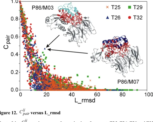
Inter-residue conservation versus L_rmsd
The pair-wise conservation score, Cijpair, between all the models within each of the CAPRI targets T25, T26, T29 and T32 have been plotted versus the corresponding L_rmsd values in Figure 12. As expected, Cijpair rapidly decreases as the L_rmsd increases, with Cijpair approaching to zero at L_rmsd higher than 30-40 Å. The Cijpair distribution is significantly spread out, even at Cijpair values around 0.5 (which means that one out of two contacts at the interface is conserved in the two considered models), and several outliers are indeed observed that contemporarily show either low
ij pair
C and low L_rmsd values or high Cijpair and high L_rmsd values. As an
example, the 3D representation of the models M03 and M07 submitted by the P86 predictor for T26, responsible for the point outlined by the arrows, is shown in the same Figure. The L_rmsd for their superimposition is as high as 19.6 Å, notwithstanding a pair-wise conservation score Cijpair of 0.47 is calculated. This is due to a significant conformational change undergone by both the receptor and the ligand in the two models (RMSD for the best superposition of the two receptors and
the two ligands is 4.8 Å and 2.8 Å, respectively), which causes a remarkably different orientation of the ligand. Nevertheless, regions involved in the interaction are substantially the same, because the ligand somehow “follows” the receptor in its conformational change. This case and many others demonstrate once more that the RMSD cannot be selected as the only descriptors for the similarity of two docking solutions and that descriptors directly describing the property of interest, in this case the interface, should be used 50,102,104,105.
Figure 12. Cijpairversus L_rmsd
Chart of the Cijpair values versus L_rmsd values for targets T25, T26, T29 and T32. A comparison of the M03 and M07 models submitted by the P86 predictor for T26 and corresponding to the point indicated by the arrows is also shown with the ligand coloured in cyan and blue, respectively; residues involved in the contacts common to the two models are shown as red sticks.
Conservation and Consensus maps for the multiple solutions submitted by each predictor
Conservation scores have also been calculated for each set of ten models submitted for each CAPRI target by the same predictor. C30, C50 and C70 (data not showed).
50% and 70% of the models, respectively. The average Cavpair and the quality score, Q-score, for each predictor, obtained on the basis of the CAPRI assessment, are also reported.
As expected, the inter-residue conservation rate within each set of multiple solutions submitted by each predictor is very variable. As an illustrative example, in Figure 13a-b, the graphical CONS-COCOMAPS outputs (consensus maps) are shown for the set of ten predictions submitted by predictors P04 and P49 for target T32. For comparison, the intermolecular contact map for the native structure (PDB code 3BX1120) is also reported (Figure 13c). The calculated Cavpair values are 0.003 and 0.400 for predictors P04 and P49, respectively. Visual inspection of Figure 13a-b immediately indicates that the solutions proposed by predictor P49 are very conservative as concerns the predicted inter-residue contacts, whereas the predicted inter-residue contacts in the solutions proposed by predictor P04 are extremely diverse and spread out all over the map. Further, the maps of Figure 13b-c also immediately show that the consensus contact map of predictor P49 is extremely similar to the contact map of the native complex structure. In fact, predictor P49 performed very well in this test case, having one acceptable, two medium quality and five high quality predictions. On the contrary, predictor P04 had only incorrect predictions.
Figure 13. Consensus maps
a-b) CONS-COCOMAPS consensus maps obtained from the 10 models submitted for the CAPRI target T32 by the P04 and P49 predictors. c-j) Comparison between the CONS-COCOMAPS consensus maps (d,f,h,j) obtained from all the 300, 310, 350 and 350 models submitted to CAPRI for the targets T25, T26, T29 and T32, respectively, and the intermolecular contact maps (c,e,g,i) of the corresponding native structures (PDB codes: 2J59, 2HQS, 2VDU and 3BX1).
We noted that there is indeed a nice correlation, especially for targets T26 and T32, between the success of the predictor and a high conservation of the inter-residue contacts. However, it is worth to remark that the opposite does not hold true, i.e. we also observed cases where a predictor submitted very similar predictions in terms of inter-residue contacts but they were far away from the native structure. For instance, the ten predictions submitted by predictor P89 for target T25 share an average Cavpair as high as 0.772, notwithstanding all the predictions have been assessed as incorrect.
The corresponding consensus map is shown and compared with the native structure contact map in the Figure 14.
Figure 14. Consensus map from the P89 predictor for T25.
Comparison between the CONS-COCOMAPS consensus map (b) obtained from the 10 models submitted for the CAPRI target T25 by the P89 predictor, and the intermolecular contact map (a) of the corresponding native structure (PDB code: 2J59).
Consensus maps for the multiple solutions submitted by all the predictors
Overall conservation scores of the inter-residue contacts in all the models submitted for the analysed targets are quite low. Conservation scores at 5, 10, 15 and 20 % are reported in Table 2, both for all the docking models and for only the incorrect solutions. They correspond to the number of inter-residue contacts which are conserved in 5, 10, 15 and 20 models out of 100, divided by the average number of contacts per model. From Table 2 it is apparent that the conservation of inter-residue contacts in T24, T28, T29 and T36 is particularly low. The conservation score of contacts common to the 5% of all the models, including the correct ones, is indeed below 0.7 (0.398, 0.056, 0.176 and 0.643, respectively). At higher percentages the conservation scores for these targets are zero, with the only exception of T36, whose C10 value is 0.016.
On the contrary, C5 assumes higher and similar values for the other three targets, from 2.274 for target T32 to 2.455 for target T25. These values are remarkably lower when the correct predictions are excluded from the analysis. C10 values are also quite similar and range from the 0.420 for target T32 to 0.576 for target T26. C15 values
are more variable, ranging from 0.078 for target T25 to 0.183 for target T26. Exclusion of the correct predictions causes a dramatic decrease of the C15 values, which approach to zero. At percentages of 20% or more, the conservation score is not higher than 0.027 for any of the analysed targets.
Target Nt C5 C10 C15 C20 T24 15818 0.398 0.000 0.000 0.000 T24-incorrect 15618 0.322 0.000 0.000 0.000 T25 15399 2.455 0.448 0.078 0.000 T25-incorrect 13613 1.477 0.020 0.000 0.000 T26 22063 2.318 0.576 0.183 0.020 T26-incorrect 19825 2.019 0.125 0.014 0.000 T28 29360 0.056 0.000 0.000 0.000 T29 23890 0.176 0.000 0.000 0.000 T29-incorrect 22923 0.000 0.000 0.000 0.000 T32 25859 2.274 0.420 0.081 0.027 T32-incorrect 23420 1.754 0.202 0.027 0.000 T36 12750 0.643 0.016 0.000 0.000 T36-incorrect 12673 0.628 0.016 0.000 0.000 a Calculations performed upon excluding all the correct predictions.
Table 2.
Inter-residue conservation scores at different percentages for all the models submitted for each target.