Chapter 5
Redistribution of Torque
In our model we analyzed the effects of the engine torque redistribution between rear and front axle to study the feasibility of a new stability control system, or to improve perfor-mance of traditional ESP’ s. The natural oversteer-understeer of a vehicle is due to many different factors: vertical load distribution between front and rear axle, tyre characteristic, engine torque flow, suspension geometry and stiffness, etc. In particular the drive torque flow, on account of the typical tyre behavior, makes the vehicle inclined to be oversteering if the torque is directed towards the rear axle. On the other hand a front-wheel drive car is inclined to be understeering. This fact does not mean that necessarily a front-wheel drive vehicle is oversteering and the contrary for a rear-wheel drive car, by reason of the several factors affecting the vehicle behavior. However considering two cars which are different just in the drive torque distribution (as we did in our research) we can say that the front-wheel drive vehicle is “more understeering” than the rear-wheel drive car (but for example both of them can be oversteering). In order to give an intuitive explanation of the reason of the different behavior we illustrate a simple, but not rigorous demonstration.
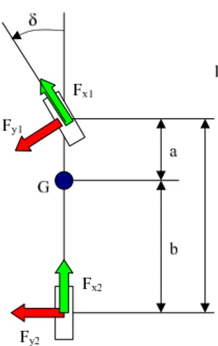
We consider a “Single Track Model” (5.1) with linear tyres ( [6], [11]), in order to schema-tize a front-wheel drive car and a rear-wheel drive car, both with the same characteristic dimensions.
Starting from the balance equations we can calculate the curve radius the car drives along in steady state conditions
Rss= u rp = 1 δ(l − ( C1a − C2b C1C2 ) mu2 l ) 1 (5.1)
1This equation (as remarked in [6]) is valid for a rear-wheel drive car, but can be acceptable to model
a front-wheel drive car if the steer angle is small enough, so in the following demonstration we accept this simplification.
Figure 5.1: “Single Track Model” scheme
C1,2 are the equivalent cornering stiffnesses of the front and rear axles. As explained in
the second chapter the longitudinal forces transferred by a tyre influence the lateral forces, but the linear model does not take this fact into account. We can imagine to approximate combined slip conditions reducing the cornering stiffness, multiplying it by a positive factor lower than 1 ((1 − ε) and (1 − γ)). Considering a car equipped with the same type of tyre in the front and in the rear axle, producing an axle cornering stiffness equal to C we obtain (with the subscript f we refer to the front-wheel drive car and with the subscript r we refer to the rear-wheel drive car)
Rss,f = u rp = 1 δ(l − ( C(1 − ε)a − Cb (C(1 − ε))C ) mu2 l ), 0 < ε < 1 (5.2) Rss,r = u rp = 1 δ(l − ( Ca − C(1 − γ)b C(C(1 − γ)) ) mu2 l ), 0 < γ < 1 (5.3)
Considering for both the cars the same longitudinal speed (u) and the same steer angle (δ), we calculate Rf − Rr, and we achieve the following result
Rf − Rr = mu2 l (− C(1 − ε)a − Cb C2(1 − ε) + Ca − C(1 − γ)b C2(1 − γ) ) = = mu 2 l ( b(1 − γ)ε + a(1 − ε)γ C(1 − ε)(1 − γ) ) (5.4)
In (5.4) both the numerator and the denominator are greater than zero, then Rf− Rr >
0, whatever are the values of ε and γ (included within the limits mentioned above). It 38
means Rf > Rr, that is to say the front wheel drive car drives along a wider bend than
the rear-wheel drive car.
We can try to understand the reason of the different behavior also during a transitory, for example considering a manoeuvre in which the steer angle follows a step function with null initial value. In fact when it passes from zero to another value only the front wheel has a slip angle different from zero (exactly equal to the steer angle), but α2 = 0, hence
Fy2 = 0. For the balance equation
J˙r = Fy1a − Fy2b (5.5)
We obtain (giving the two cars the same steer angle also in this case) a front wheel-drive car that has a yaw acceleration lower than the rear-wheel wheel-drive car. It means that, supposing the two cars running at the same longitudinal speed, at least during the first instants Rf will be wider than Rr.
Our idea was to try to transfer torque to the front axle in case of excessive oversteer, and contrary to provide torque to the rear axle if an excessive understeer is detected. This system cannot replace an ESP system completely because for example if it is applied on a front-wheel drive car, it can be able only to correct understeer, but to correct an oversteering behavior a traditional ESP remains necessary. The opposite occurs for a rear-wheel drive vehicle.
5.1
Drive Torque Control
Since the vehicle we modelled is supplied with an “Haldex” coupling we can only intervene on the internal valve position to govern the engine torque flow.
5.1.1
Controller
To control the valve we used the same quantities as in the ESP. If the PI controller output exceeds a threshold value we close completely the valve, therefore we transfer the maximum possible amount of torque (depending on the working point on the coupling characteristic), otherwise we keep the valve open, and no torque is transferred (fig.5.2). The threshold magnitude for the valve controller is lower than the correspondent value for the ESP. Initially we want to control the car motion acting on the distribution of torque, and only if this intervention is not effective we activate the brake system. As long as possible in fact we
want to avoid to apply a brake torque. The simulations confirm that the ESP intervention is very powerful but also uncomfortable, and it makes the vehicle performances worse.
Figure 5.2: “Redistribution of Torque” controller subsystem
We prefer to use a control which opens or closes completely the valve without any possible intermediate position because the redistribution of torque exploits an amount of drive torque, and whereas its value is not usually very big (in comparison for example with the brake torque applied by the ESP), the whole available torque must be applied to obtain performances as strong and quick as possible, without risking to overcompensate the undesired behavior.