3 The Minimum 1-D model
3.1 The concept of the Minimum 1-D model
Solutions of three-dimensional seismic tomography, obtained by solving the coupled hypocentre locations-velocity model inverse problem, highly depend on the data quality and on the 1-D reference velocity model (Kissling et al., 1994). Consequently, for the tomographic images resulting from three-dimensional inversion, an appropriate initial velocity model should be used. Kissling et al. (1994), to find the best initial reference model for LET, introduced the concept of the minimum 1-D model.
The minimum 1-D model itself is the result of a series of simultaneous inversions of hypocentral parameters, 1-D velocity models (Vp and Vs) and station corrections. In the 1-D
minimum model, the velocity of a given layer of the is to be considered as the best average of the lateral velocities that belong to the layer.
Moreover, the precision of routine earthquake location is strictly linked to the kind of velocity model used. Besides serving as an initial reference model for LET, the minimum 1-D model, provides high precision hypocentre locations. With this velocity model, all earthquakes used in the 1-D inversion and also required in the successive step of LET show a minimum average of rms value.
The dependence of the 3-D inversion on the reference model is a problem that has to be addressed in any application of seismic tomography. In fact, not only an inappropriate initial reference model affect the quality of the 3-D image by introducing artefacts, but it may underestimate the uncertainties of the results (Kissling et al., 1994).
In this chapter, an application of the method proposed by Kissling et al. (1994) is presented to compute a 1-D model that is used as a reference model for 3-D seismic tomography and for routine earthquake location in Lesser Antilles region. Following the mentioned method, the travel time data, together with revised hypocentre coordinates and station corrections, are jointly inverted to obtain the “Minimum 1-D model”. As data quality is of great importance for success and accuracy of the inversion process, for the Minimum 1-D computation we use earthquakes after a careful selection, previously described in chapter two. Successively, the obtained earthquake locations are tested and compared to the ones
derived from the a-priori models proposed. Finally (see chapter four), the 3-D tomographic inversion is determined using the minimum 1-D as the starting P- and S-wave velocity model.
.
3.2 Coupled hypocentre Velocity Model Problem
The arrival time (t) of a seismic wave generated by an earthquake is a non-linear function of the station coordinates (s), the hypocentral parameters (h) and the velocity model (m):
tobs = f (s, h, m). (1)
Generally, neither the true hypocentral parameters nor the velocity model are known, therefore it is impossible to solve directly the equation (1) with arrival times and station locations, the only measurable quantities. To proceed, we have to make a guess of the unknown parameters. Using an a-priori velocity model, we trace rays from a trial source location to the receivers, with calculated theoretical arrival times (tcalc). Then, the residual
travel time (tres) that is the difference between the observed and the calculated travel time (see
chapter one), can be expanded as a function of the differences between the estimated and the true hypocentral and velocity parameters. To compute suitable adjustments (corrections) to the hypocentral and model parameters, we need to know the dependence of the observed travel times on all parameters.
Applying a first-order Taylor series expansion to equation (1), we obtain a linear relationship between the travel time residual and adjustments to the hypocentral (Dhk) and velocity (Dmi) parameters:
1, 4 1,
k
res obs calc k i i
k i f f t t t h n m e h m ¶ ¶ = - = = D + = D + ¶ 
å
å
(2)The coupled hypocentre-velocity model parameter can also be written, in a matrix notation as: t = Hh + Mm + e = Ad + e (3)
where:
t = vector of travel time residuals;
H = matrix of partial derivatives of travel time with respect to hypocentral parameters; h = vector of hypocentral parameter adjustments;
M = matrix of partial derivatives of travel times with respect to model parameters; m = vector of velocity parameter adjustments;
e = vector of travel time errors, including contributions from errors in measuring the observed travel times, errors in tcalc due to errors in station coordinates, use of the wrong velocity model
and hypocentral coordinates, and errors caused by the linear approximation; A = matrix of all partial derivatives;
d = vector of hypocentral and model parameter adjustments.
In a standard earthquake location, the velocity parameters are maintained fixed to a-priori values and the observed travel times are minimized by perturbating the four hypocentral parameters. Precise hypocentre locations and error estimate, therefore, demand the simultaneous solution of both velocity and hypocentral parameters. Kissling et al. (1994) concur with Thurber (1983) that the correct hypocentral coordinates are most reliably achieved by solving the coupled hypocentre-velocity model problem, rather than alternating independent hypocentre and velocity adjustment steps.
The obtained minimum 1-D model represents a velocity model that reflects the a-priori information and that leads to a minimum average of rms values for the best selected earthquakes used in the inversion.
Each velocity layer of the minimum 1-D model is the weighted area wise average over all rays in the data-set within that depth interval. To account for lateral variations in the shallow subsurface, station corrections are included in the 1-D inversion process.
3.3 The search of the Minimum 1-D Model
Simultaneous inversions of hypocentral parameters, velocities and station corrections were performed by using the VELEST software (Kissling, 1995). This program is a FORTRAN77 routine that is designed to derive 1-D velocity models for earthquake location procedures and as initial reference models for seismic tomography.
This step is very important because tomography is based on the linearization of a non-linear function that relates travel times to unknown parameters. To be allowed to perform the linearization, a-priori parameters must be introduced and these a-priori parameters should be
close enough to the true ones. The relation between the parameters and the travel times is highly non linear. The goal of the 1-D inversion is therefore, to explore the parameters space and to find a good starting point for the successive step of the 3-D inversion.
The goodness of a starting model can be decided by comparing, for the selected events used in the D inversion, the a-priori rms to the final rms, obtained by using the minimum 1-D model. If the residual decreases, it means that the obtained 1-1-D model was able to explain part of residuals. The remaining residuals are to be explained by lateral velocity heterogeneities during the 3-D inversion step.
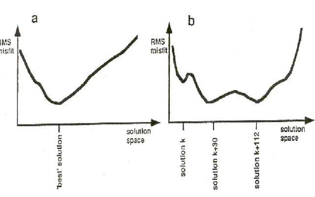
The best solution to the coupled hypocentre-velocity model problem of the Minimum 1-D model consists of a combination of hypocentres, velocity model and station corrections. Considering any possible combination of hypocentres, velocity models and station corrections, the solution to the mentioned problem is the minimum value of rms misfit (figure 3.1).
Figure 3.1: Quality estimate of solutions to the coupled problem. A: Simple case with unique solution. B: Normal case with several minima of rms misfit. The diagram displaying the rms misfit most probably looks more like figure 3.1b. Modified from Kissling (1995).
Unfortunately, in the case of the coupled problem with local earthquake data, such diagram displaying the rms misfit most probably looks more like figure 3.1b, where several local rms misfit minima occur and we do not know this function a-priori. For this reason, we must search for different solutions with minimal rms misfit by varying initial models and hypocentre locations. This way, the search of a minimum 1-D model amounts to a trial-and-error process, performed by VELEST. Therefore, the search of the minimum 1-D model starts with a wide range of realistic wave velocity models. Layers with constant velocity constitute these models. Inversion of hypocentral parameters and velocities is done jointly and iteratively.
The concept of the minimum 1-D model includes station corrections relative to the velocity of the upper layers and the reference station. Station corrections are an integral part of the 1-D velocity model since they should at least partly account for the overall three-dimensionality of the velocity field, in particular the structure that may otherwise not adequately be represented by a 1-D model (Kissling et al., 1995). In fact there is no rays-crossing just below the site of station, so it makes no sense to average the site heterogeneities to constrain the upper layers. Part of the residuals not explained by the 1-D structure will be included into these station corrections. Furthermore, these corrections give an idea about the superficial geology and lead to a first insight into the 3-D structure under investigation.
Figure 3.2: It can clearly be seen that the raypath lengths for all of these shallow events are more or less similar in layer 1, whereas in other layers the raypath lengths show much larger variation (From Haslinger, 1988).
That station corrections are strongly coupled to the velocities and to the structure of the upper layers can easily be understood if one realizes that the ray lengths in the upper layers for one station normally are similar for all rays to the station, whereas in other layers the individual ray lengths are much more different (Haslinger, 1988) (figure 3.2). So again, a change in velocity structure of the upper layers translates into a more or less constant time-shift for all calculated travel times, which in turn can be compensated by adjusting the station correction.
Therefore, if we have, as for the SISMANTILLES I data, many deep seismic events this reasoning holds of course not only for the upper layers but for the whole set of layers where raypaths are more or less sub-vertical. Consequently the important parameter for interpreting the station corrections is the relative difference between them, which can be compared to the 1-D structure and to the geological near-surface conditions of the area under study.
The station correction is supposed equal to 0 at the site of reference station and all other site delays are computed relatively to this. A reference station makes the link with the first layer and should show the three following features:
- It should lie toward the middle of the network;
- It should show a large number of readings with high observation weights;
- It should not be situated in an area with unknown surface geology or at the border between two units with strongly different geology.
VELEST allows to use station elevations for the mentioned joint inversion of hypocentral and velocity parameters. When using station elevations, rays are traced exactly to the true station position. This is an important constrain for this work, ranging the station elevations from 4000 m below sea level to over 1300 m above.
3.4 Details about the use of VELEST software
Following the recommendations of Kissling et al. (1994), we began the 1-D inversion process with a large number of thin layers and combined layers where velocities converged to similar values during the inversion process. The output file (.cnv) of VELEST single-event
mode become the input file to the same software but in simultaneous mode (figures 3.3 and 1.18).
VELEST program now runs in a mode that computes the minimum 1-D model with station delays and relocates the events.
The a-priori models provided to VELEST must be built on a-priori knowledge of the structure under investigation. However, it is necessary to try different variant of a-priori 1-D model to avoid the push of the solution to a local minimum (Fig. 3.1). The following draft summarizes all the input and output files (tables 3.1, 3.2, 3.3, 3.4 and 3.5) of VELEST in a simultaneous mode:
Velest in a simultaneous mode
1D a-priori velocity model
file.mod
New velocity model,
new stationslist with delays
new summary cards
file.VEL
Station coordinates
file.sta
Control parameters
file.cmn
Earthquake phases
file.cnv
Figure 3.3: How VELEST runs in a “simultaneous mode”: input and output files.
Several runs of VELEST need to constrain the minimum 1-D model. The control file .cmn allows to “play” with switches, in the following tables we can see examples of the files used in our work, for details on each switch you can see the VELEST user’s guide (Kissling, 1995).
olat olon icoordsystem zshift itrial ztrial ised +16.2323 61.4942 0 0.000 0 25.00 0
***
*** neqs nshot rotate 155 0 0.0
***
*** isingle iresolcalc 0 0
***
*** dmax itopo zmin veladj zadj lowveloclay 500.0 0 -1.2 0.2 8.00 0
***
*** nsp swtfac vpvs nmod 2 0.60 1.750 2
***
*** othet xythet zthet vthet stathet 0.01 0.01 0.01 1.0 0.01
***
to be continued ………
******* END OF THE CONTROL-FILE FOR PROGRAM V E L E S T ******* Table 3.1: Example of the input control file .cmn.
10 vel,depth,vdamp,phase (f5.2,5x,f7.2,2x,f7.3,3x,a1) 3.50 -3.0 001.00 P-VELOCITY MODEL 6.00 3.0 001.00 6.00 6.0 001.00 6.00 9.0 001.00 6.00 12.0 001.00 7.00 15.0 001.00 to be continued ………
Table 3.2: Example of the input file .mod with regards the a-priori velocity model.
2 125 1634 20.81 16.8195N 61.6737W 12.47 3.00 130 0.36
HYP P0 8.05BARBS0 20.49BARBP0 11.48BLMAS1 20.84BLMAP0 11.64BOG S1 10.65 BOG P0 6.08CAGZP3 13.84CELCS0 21.02CELCP0 11.63-DANJS0 17.53-DANJP0 9.77 DEGZP3 13.47DEGZS3 23.94DOGZP2 14.57FNGZP2 14.10FRE S0 9.61FRE P0 5.36
j02 P0 8.16j02 S0 15.14j18 S2 29.67j18 P0 16.22j20 P0 20.85MOGZP2 14.18 MONTS2 24.01MONTP1 13.50NEROS0 19.01NEROP0 10.64NTRDS2 18.10NTRDP0 10.47 PAGZP2 14.12RETRS2 20.55TASSS0 20.18TASSP0 11.34
2 125 19 0 49.21 16.8737N 60.9229W 34.71 3.00 137 0.58
DEGZP2 10.51-DEGZS3 19.60DESIP1 10.71j02 P0 6.59j04 P0 8.60MONTP0 10.66 HYP P0 11.60BARBS2 26.60BARBP1 14.68BOG S2 27.97BOG P0 15.76CELCP1 12.84 DANJP0 12.58DESIS2 19.73-DOGZP2 19.23FNGZP2 19.37FRE S1 24.47FRE P0 13.83 j02 S1 11.98j15 P0 12.82j18 P0 15.12j20 P1 18.12j22 P2 11.43j26 P3 26.98 MOGZP3 19.56MONTS2 20.03NEROS3 22.70NEROP0 12.44NTRDS2 30.09NTRDP1 17.03 TASSP0 14.15
to be continued ……… Table 3.3: Example of the input phase file .cnv.
(a4,f7.4,a1,1x,f8.4,a1,1x,i5,1x,i1,1x,i3,1x,f5.2,2x,f5.2,3x,i1) SLBZ13.8258N 61.0408W 600 1 1 0.00 0.00 1 BAMZ14.8157N 61.1483W 670 1 2 0.00 0.00 1 BIMZ14.5170N 61.0708W 425 1 3 0.00 0.00 1 BVMZ14.7350N 61.0797W 694 1 4 0.00 0.00 1 CPMZ14.8155N 61.2105W 335 1 5 0.00 0.00 1 to be continued ……… Table 3.4: Example of the input station file .sta.
Different output files may also be created by VELEST. Information about the 1-D inversion are written into these output files and among them we have:
◊ The total number of readings per station, the a-priori data variance and residual.
◊ Per iteration: the a-posteriori variance and residual, the decrease in % of variance. If the steps are large the starting point is far from a minimum.
◊ Per iteration: hypocentre parameters adjustments. As the solution converges, the adjustments should get smaller.
◊ Per iteration: new velocity model, hypocentre parameters and delays.
◊ Rays statistics: number of direct, reflected and refracted rays. Direct rays improve the quality of 3-D tomography.
◊ Layer statistics: number of hypocentre for layers, number of direct, reflected or refracted rays, the total number of rays.
◊ Distribution of final depths compared to initial depths to see how sensitive they are to the a-priori model.
◊ Residuals per station and also per azimuth: the surface of investigation is divided into four quadrants and the program computes the residuals per quadrant.
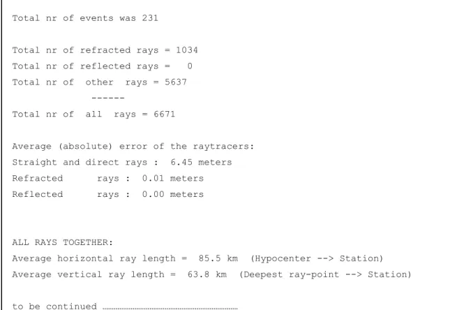
The last run of VELEST in simultaneous mode also provides some statistics about ray and layer statistics:
RAY-STATISTICS FOR L A S T ITERATION NHYP : nr of hypocentres in this layer NREF : nr of headwaves in this layer %len : % of "refracted km" in this layer with respect to all refracted kilometers NHIT : nr of rays passed thru this layer
xy-km: average horizontal ray length [km] in layer z-km : average vertical ray length [km] in layer RFLX : number of reflections at bottom of this layer
nlay top ... bottom velocity NHYP NREF %len NHIT xy-km z-km RFLX 1 -3.00... 3.00 km 3.47 km/s 2 0 0.0 6273 1.2 2.9 0 2 3.00... 6.00 km 5.86 km/s 4 35 1.4 7179 2.9 2.8 0 3 6.00... 9.00 km 6.12 km/s 4 36 1.9 6621 3.4 3.0 0 4 9.00... 12.00 km 6.26 km/s 13 3 0.2 6617 3.5 2.9 0 5 12.00... 15.00 km 6.38 km/s 3 5 0.1 6380 3.2 3.0 0 6 15.00... 18.00 km 7.06 km/s 2 159 11.3 6233 6.2 2.9 0 7 18.00... 21.00 km 7.06 km/s 13 20 1.5 6252 4.7 2.8 0 8 21.00... 24.00 km 7.33 km/s 8 170 10.4 5783 6.1 2.8 0 9 24.00... 27.00 km 7.33 km/s 16 0 0.0 5657 4.2 2.8 0 10 27.00... 30.00 km 7.33 km/s 11 0 0.0 5415 3.9 2.9 0 11 30.00... 30.00 km 8.07 km/s 0 606 73.3 0 0.0 0.0 0 12 0.00... 0.00 km 0.00 km/s 0 0 0.0 0 0.0 0.0 0 13 0.00... 0.00 km 0.00 km/s 0 0 0.0 0 0.0 0.0 0 14 0.00... 0.00 km 0.00 km/s 0 0 0.0 0 0.0 0.0 0 15 0.00... 0.00 km 0.00 km/s 0 0 0.0 0 0.0 0.0 0 16 0.00... 0.00 km 0.00 km/s 0 0 0.0 0 0.0 0.0 0 17 0.00... 0.00 km 0.00 km/s 0 0 0.0 0 0.0 0.0 0 18 0.00... 0.00 km 0.00 km/s 0 0 0.0 0 0.0 0.0 0 19 0.00... 0.00 km 0.00 km/s 0 0 0.0 0 0.0 0.0 0 20 0.00... 0.00 km 0.00 km/s 0 0 0.0 0 0.0 0.0 0 21 0.00... 0.00 km 0.00 km/s 0 0 0.0 0 0.0 0.0 0 22 0.00... km 0.00 km/s 155 0 0.0 0 0.0 0.0
Total nr of events was 231
Total nr of refracted rays = 1034 Total nr of reflected rays = 0 Total nr of other rays = 5637
Total nr of all rays = 6671
Average (absolute) error of the raytracers: Straight and direct rays : 6.45 meters Refracted rays : 0.01 meters Reflected rays : 0.00 meters
ALL RAYS TOGETHER:
Average horizontal ray length = 85.5 km (Hypocenter --> Station) Average vertical ray length = 63.8 km (Deepest ray-point --> Station) to be continued ………
Table 3.5: The main VELEST output file .VEL
In this inversion process, where we decided that the output files (velocity model, hypocentre parameters, station delays) must be supplied to the successive run, we established a succession runs composed of a definite number of iterations.
The criteria that will stop the iterations are the following: ◊ The rms diminution is large enough.
◊ The hypocentre adjustments are stable through-out the iterations. The quality of the obtained minimum 1-D model can be evaluated by:
◊ Comparing the results derived from the inversion process applied to different a-priori models. If from very different a-priori models we obtain very similar minimum 1-D models, our solutions are robust.
◊ Comparing the final 1-D model with station corrections to a-priori knowledge of the structure available.
◊ Comparing the rms distribution with that obtained from the a-priori model.
Once the minimum 1-D model is computed, our data-set of 155 seismic events are again supplied to VELEST single-event mode, that allows us to obtain a not simultaneous
relocation of the selected earthquakes that will be read, in step 3, by SIMULPS14 (Evans et al., 1994,Eberhart-Phillips, 1989) (Fig. 1.11).
3.5 1-D inversion of the SISMANTILLES I data-set
With regards to the area under study, the identification of the minimum 1-D model has been carried out after a careful filtering of data with respect to their quality (see chapter two). We obtained a data-set of 155 well-locatable seismic events with a total of 4,054 P-observations and 2,617 S-P-observations. All S-phases were picked on the horizontal components of the three-component stations; this explains the smaller number of S-picks.
For the 1-D inversion we used two a-priori models (figure 2.4), S-phases were included in the inversion procedure by assuming a constant Vp/Vs ratio of 1.76, derived by Wadati diagrams (Clément, 2001). The inversion was stopped when the earthquake locations, stations delays and velocity values did not vary significantly in subsequent iterations. In particular, the steps that lead to the final models consist of two runs. First of all, both hypocentre locations as velocity structure are inverted, using the global misfit as a measure for the goodness of fit. In a second run we maintain fixed the obtained velocity model and both hypocentre locations as station corrections are inverted. Because station corrections are an integral component of the velocity model and partly account for the overall tree-dimensionality of the velocity field, adopting this procedure we have a more homogeneous comparison between velocity models obtained from the inversion of the two different starting structures.
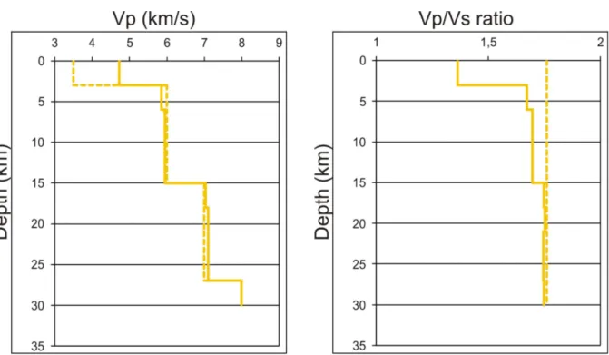
Figure 3.4: Starting 1-D P-wave velocity model named Model 1 (dashed line) and the computed Minimum 1-D velocity model (continuous line). On the right the Vp/Vs ratio.
With a total of 920 unknowns (4 x 155 hypocentral parameters, 20 velocities, and 280 station corrections) and 6,671 observations, the over-determination factor of the inverse problem is approximately 7.25. The derived minimum 1-D velocity structures (continuous line) are shown in figures 3.4, and 3.5 together with each start model (dashed line).
Figure 3.5: Starting 1-D P-wave velocity model named Model 2 (dashed line) and the computed Minimum 1-D velocity model (continuous line). ). On the right the Vp/Vs ratio.
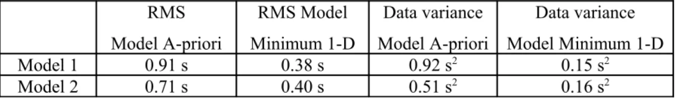
As we can see also from table 3.6, the average travel time residuals for the start models was reduced, after the inversion process, to over 40 %. Also the data-variance value decreased from an average of 0.70 s2 to over 70%. In order to verify if our computed models
improve earthquake location quality, we plot the rms value for the 155 selected after each run of the 1-D inversion process.
RMS Model A-priori RMS Model Minimum 1-D Data variance Model A-priori Data variance Model Minimum 1-D Model 1 0.91 s 0.38 s 0.92 s2 0.15 s2 Model 2 0.71 s 0.40 s 0.51 s2 0.16 s2
Table 3.6: Mean rms value and data variance of the two velocity model used
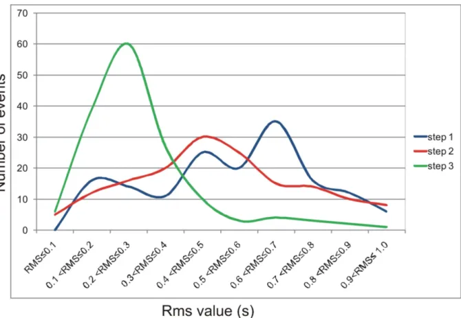
The figure 3.6 is very interesting, as it shows the rms distribution of the 155 selected events after the simple location with the a-priori (step 1), the inversion without considering station corrections (step 2) and the inversion performed considering station delays (step 3). The rms distribution, after each step, demonstrates once again that the new 1-D models and stations delays were able to explain part of the residuals. We observe that the decrease of rms value is stronger after the second run where the inversion process is designed to obtain station correction terms. These results can be explained by the huge structural heterogeneity of the central Lesser Antilles subduction zone which cannot be adequately represented by a simple P- and S-wave velocity model of about ten homogeneous layers.
Figure 3.6: Difference in rms distribution between the first earthquake location with the a-priori Model 1 (blue) and the relocation with the computed 1-D model after the two runs of the 1-D inversion process (red and green). Note the consistent decrease in rms value that indicates a good improvement of the solutions.
The obtained two P-wave minimum 1-D models show strong discontinuities for the depth of 3 and 15 km. We observe, also, a not negligible convergence of the different models that indicates a good resolvability of the 1-D structure of Lesser Antilles zone by this data-set. Indeed if the starting model, under 15 km depth, denotes P-wave velocity of 8 km/s we note in the resulting minimum 1-D a decrease. On the contrary, if the starting model, as in the case of the model 2, indicates a P-wave model of 7 km/s we note in the resulting minimum 1-D an increase. For the layers above 27 km depth we observe in the starting models a maximal difference of 1 km/s, on the contrary in the derived minimum 1-D models this maximal difference is of 0.7 km/s.
In our work we obtain also Minimum 1-D S- wave velocity models. Gomberg et al. (1990) demonstrated that partial derivatives of S-wave travel times are always larger than those of P-waves by a factor equivalent to Vp/Vs and that they act as an unique constraint
within an epicentral distance of 1.4 focal depth. The use of S-waves will in general result in a more accurate hypocentre location, especially regarding focal depth. On the other hand, a
mispicked S-arrival time at a station close to the epicenter can result in a stable solution with a small RMS value, but actually denoting a significantly mislocated hypocentre even for cases with excellent azimuthal station coverage. Since the onset of S-phases is often masked or distorted by P-wave coda, mispicking is more likely to occur with S-phases and a rigorous quality control is needed, as has been described in the previous chapter. In general, S-phases are included in the location procedure by simply assuming a constant Vp/Vs ratio. By synthetic
testing, Maurer et Kradolfer (1996) demonstrated that focal depth errors obtained with fixed Vp/Vs ratio are nearly twice as large as the errors using P- phases only. Using an independent S-wave velocity yielded the best results.
In figures 3.4 and 3.5, we show the resulting Vp/Vs values. Under 3 km depth Vp/Vs
values range from 1.65 to 1.85, above 3 km depth the values of 1.65 for the model 2 and of 1.40 (clearly unrealistic) for the model Model 1 should be considered together to the station corrections that are linked to the superficial geology (see paragraph 3.3).
To partly estimate the huge structural heterogeneity of the central Lesser Antilles region, the minimum 1-D model is complemented by station corrections that take into account near surface velocity heterogeneity and the geometry of the crust.
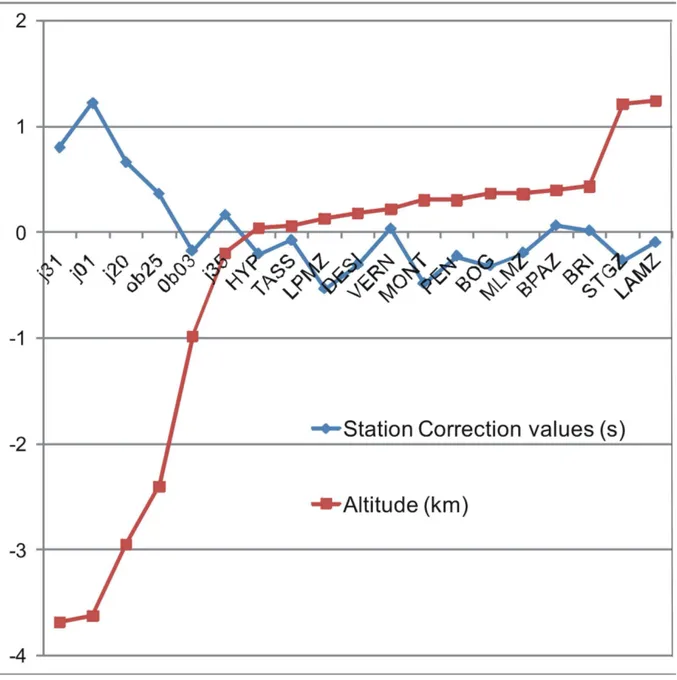
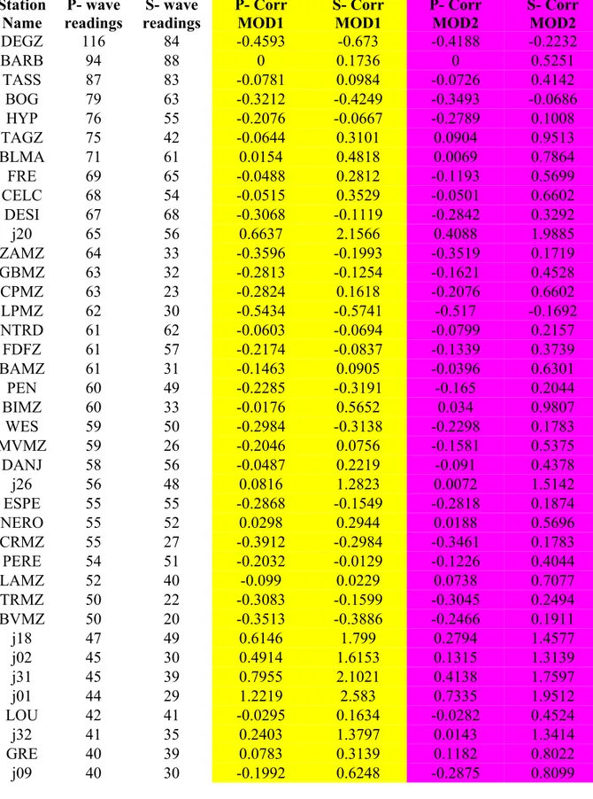
The station correction values are referred to “reference station” of BARB located in Guadeloupe Island that is among the stations with the highest number of readings. Negative corrections are encountered when the true velocities are supposed to be higher, positive correction occur for lower velocities than predicted by the model. We may exclude biases on the station corrections due to topographic effects since VELEST allows to use station elevations for the joint inversion of hypocentral and velocity parameters (figure 3.7). Consequently rays are traced exactly to the true station position (Husen et al., 1999)
Figure 3.7: Elevation (km) and correction term values of some seismic stations of SISMANTILLES I experiment. We exclude biases on station correction values since VELEST takes into account station altitude for the simultaneous 1-D inversion.
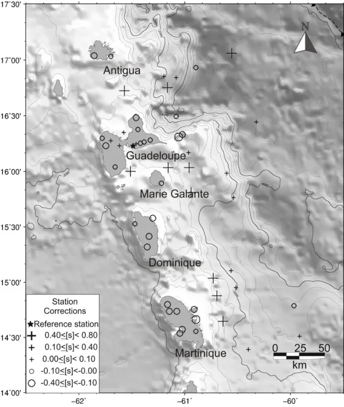
We obtained, from 1-D inversion, a correction value for all station positions. In figure 3.8 and table 3.7, we plotted the P station-terms with a large number of observations (over 40); this guarantees that 3-D effects on the source-station raypaths compose a well-controlled average, and that the relative differences in station-terms are meaningful in terms of 3-D interpretation. For the land stations, the station-terms retrieved by the inversion show a trend of small positive or small negative values in the Guadeloupe and Marie Galante Islands, negative values in Antigua and Dominique islands and larger negative values in Martinique Island.
This variation could not have been anticipated independently, such as from consideration of surface geology.
Figure 3.8: Station corrections computed with the minimum 1-D velocity model (model 2). Crosses indicated positive and circles negative delays with respect the reference station. The relative difference between station corrections leads to a first insight in the deeper 3-D structure.
Station Name P- wave readings S- wave readings P- Corr MOD1 S- Corr MOD1 P- Corr MOD2 S- Corr MOD2 DEGZ 116 84 -0.4593 -0.673 -0.4188 -0.2232 BARB 94 88 0 0.1736 0 0.5251 TASS 87 83 -0.0781 0.0984 -0.0726 0.4142 BOG 79 63 -0.3212 -0.4249 -0.3493 -0.0686 HYP 76 55 -0.2076 -0.0667 -0.2789 0.1008 TAGZ 75 42 -0.0644 0.3101 0.0904 0.9513 BLMA 71 61 0.0154 0.4818 0.0069 0.7864 FRE 69 65 -0.0488 0.2812 -0.1193 0.5699 CELC 68 54 -0.0515 0.3529 -0.0501 0.6602 DESI 67 68 -0.3068 -0.1119 -0.2842 0.3292 j20 65 56 0.6637 2.1566 0.4088 1.9885 ZAMZ 64 33 -0.3596 -0.1993 -0.3519 0.1719 GBMZ 63 32 -0.2813 -0.1254 -0.1621 0.4528 CPMZ 63 23 -0.2824 0.1618 -0.2076 0.6602 LPMZ 62 30 -0.5434 -0.5741 -0.517 -0.1692 NTRD 61 62 -0.0603 -0.0694 -0.0799 0.2157 FDFZ 61 57 -0.2174 -0.0837 -0.1339 0.3739 BAMZ 61 31 -0.1463 0.0905 -0.0396 0.6301 PEN 60 49 -0.2285 -0.3191 -0.165 0.2044 BIMZ 60 33 -0.0176 0.5652 0.034 0.9807 WES 59 50 -0.2984 -0.3138 -0.2298 0.1783 MVMZ 59 26 -0.2046 0.0756 -0.1581 0.5375 DANJ 58 56 -0.0487 0.2219 -0.091 0.4378 j26 56 48 0.0816 1.2823 0.0072 1.5142 ESPE 55 55 -0.2868 -0.1549 -0.2818 0.1874 NERO 55 52 0.0298 0.2944 0.0188 0.5696 CRMZ 55 27 -0.3912 -0.2984 -0.3461 0.1783 PERE 54 51 -0.2032 -0.0129 -0.1226 0.4044 LAMZ 52 40 -0.099 0.0229 0.0738 0.7077 TRMZ 50 22 -0.3083 -0.1599 -0.3045 0.2494 BVMZ 50 20 -0.3513 -0.3886 -0.2466 0.1911 j18 47 49 0.6146 1.799 0.2794 1.4577 j02 45 30 0.4914 1.6153 0.1315 1.3139 j31 45 39 0.7955 2.1021 0.4138 1.7597 j01 44 29 1.2219 2.583 0.7335 1.9512 LOU 42 41 -0.0295 0.1634 -0.0282 0.4524 j32 41 35 0.2403 1.3797 0.0143 1.3414 GRE 40 39 0.0783 0.3139 0.1182 0.8022 j09 40 30 -0.1992 0.6248 -0.2875 0.8099
Table 3.7: List of station corrections terms with regard land stations and OBS with at least 40 P-wave observations.
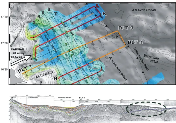
With regards OBS station corrections, SISMANTILLES I experiment provides a rare opportunity to check the efficiency of the minimum 1-D inversion scheme. In particular we retrieve station-correction values that are meaningful in terms of the local structure under the stations which is usually not known independently. Indeed the OBS station-terms are in general positive with respect to land stations indicating late arrivals, consistently with the presence of soft mud and sediments at the sea-bottom, and they vary with their thickness as can be derived here from multi-channel reflection seismic (MCS) profiles shot over them (Laigle et al., 2011). Figure 3.9 shows two dip-line transects revealed by this MCS imaging performed, during the year 2007, in context of the SISMANTILLES II experiment.
Figure 3.9: Two dip-line transects (DLT 1 and DLT 2) revealed by MCS imaging performed in context of the SISMANTILLES II experiment. On the arcward side the thick sedimentary deposit within the forearc basin (4 s ~ 5 km below sea level) is marked by green line. The sediment reaches a maximum thickness of 5 km. We observe also an ongoing deformation at crustal scale (dashed line) associated to the oblique subduction of Barracuda ridge. (Modified from Laigle et al. 2010).
Figure 3.10: Observing the first onset on the horizontal component that corresponds to the conversion beneath the OBS of the incoming P-wave into a S-wave at the base of the mud layer Laigle et al. (2010) determined mud layer thickness. They have assumed for mud a P-wave velocity and a Vp/Vs ratio equal respectively to 2 km/s and to 2.7.
Moreover Laigle et al. (2011) were able to validate their findings about the thickness of sedimentary deposit within the forearc basin and our results regarding station correction values. They obtain the arrival times of P-wave (Tp) and of P-wave to S-wave converted (Tps) at the base of the mud layer (figure 3.10). In a subsequent step, assuming for mud a P-wave velocity and a Vp/Vs ratio equal respectively to 2 km/s and to 2.7, they determined, under OBS position of SISMANTILLES II experiment, mud layer thickness, applying a very simple relation (figure 3.10). Finally they calculated station correction values with respect a simple model characterized by a constant P-wave velocity of 6 km/s. Figure 3.11 shows, for 17 OBS positions, the comparison between P-wave station correction values determined by Laigle et al. (2011) approach and by our Minimum 1-D model 1 correlated to mud layer thickness as determined by MCS imaging. Figure 3.12 shows the final hypocentre locations of the 155 well-locatable events in a map and three vertical cross-sections perpendicular to the arc. We were able to improve hypocentre determinations by adding S-wave readings and reducing the azimuthal gap by the OBS stations.
A comparison with other localizations obtained from other velocity models or networks will be performed in the following sections.
Figure 3.11: Comparison between P-wave stations corrections values (s) as determined by Laigle et al. (2011) (green) and after our Minimum 1-D model 2 (blue) correlated to mud layer thickness (red) under each OBS positions. Laigle et al. (2011) calculated station correction values with respect a model characterized by a constant P-wave velocity of 6 km/s. The OBS station-terms are in general positive with respect to land stations indicating late arrivals, consistently with the presence of soft mud and sediments at the sea-bottom, and they vary with their thickness.
3.6 Earthquake relocation with the computed minimum 1-D models and comparison with a-priori locations
Figure 3.13 shows the comparison, during the operating time of OBS instruments, between hypocentres located with only the permanent array data (Bengoubou-Valerius et al., 2008) and by using also the temporary deployment of OBS’s and land stations, after 1-D inversion of the Model 1. As expected, there are significant differences as a consequence of the unfavorable azimuthal coverage and of the lack of S-wave readings of the permanent IPGP seismic stations. In particular, without SISMANTILLES I data, reliable hypocentre determination is restricted to the region within the land station network.
Figure 3.12: Accurate hypocentre locations (circles) as determined by the minimum 1-D P and S-wave inversion (model 1) using a combined on-/offshore network. Earthquake localization obtained with OBS contribution are marked in black. Profiles AA’, BB’ and CC’ indicate the orientations of the cross-sections shown at the right side. The dashed line with triangles (top right corner) represents the oceanic trench. The permanent seismic stations of the IPGP observatories and the landward temporary stations are respectively represented by white diamonds and triangles. OBS positions are represented by squares. Dashed white lines are the prolongation of the two borders of the Tiburon ridge according to its trend at the deformation front, assuming a straight subducting path beneath forearc region.
Mislocations, in focal depth and epicentre, of events located without OBS and S-wave are up to 20 km. Figure 3.14 shows the epicentral map of the selected events located with the a-priori model 1 and relocated after 1-D inversion.
Figure 3.13: Comparison between earthquake locations obtained here from temporary OBS offshore and land stations (black) and from the IPGP permanent monitoring observatories (grey). A gray line represents slab position as inferred from figure 3.12.
Figure 3.14: Epicentral map of the selected located with the a-priori model 1 (yellow circles) and with its derived Minimum 1-D model (black circles). Three seismicity cross sections are taken and presented in figure 3.16. In the figure are represented stations of OVSG (blue triangles), temporary land stations (red triangles) and OBS (red squares).
Most of the events retain the position obtained with the a-priori model and only few events are affected by larger displacements. With regards to the focal depth, we noted generally a shift of the majority of the seismic events (Fig. 3.15).
Figure 3.15: Distribution of foci along profiles of Fig. 3.13. On the left we have the events located with the a-priori model 1, on the right we have the events located with the minimum 1-D model. Zero is referred to the position of the station of BARB. With regards to the focal depth, we noted generally a shift of the majority of the seismic events.
Figure 3.16: Epicentral map of the selected located the a-priori model 1 (fuchsia circles) and with its derived Minimum 1-D model (black circles). Three seismicity cross sections are taken and presented in figure 3.14. In the figure are represented stations of OVSG (blue triangles), temporary land stations (red triangles) and OBS (red squares).
Figure 3.17: Distribution of foci along profiles of Fig. 3.14. On the left we have the events located with the a-priori model 2, on the right we have the events located with the minimum 1-D model. Zero is referred to the position of the station of BARB
After the inversion process, we note, as well the velocity models represented in figure 3.4 and 3.5, a significant convergence also for hypocentral parameter. As we can see from
figures 3.18 and 3.19, the differences between longitude, latitude, depth and origin time obtained with the two a-priori models, 2 and 1, are more remarkable to those determined by using the two derived 1-D minimum model.
Figure 3.18: Differences in hypocentral parameters (longitude and latitude) between earthquake locations obtained by using the a-priori (blue) velocity model (1 & 2) or the derived minimum 1-D (red).
In longitude, the pattern the majority of events is dominated by the great limitation of the shifts toward east, on the contrary in latitude there is a reduction of the shift toward north and south. The shift in depth can be mostly attributed to the differences in the velocity models: there is no difference under 30 km depth where the two minimum 1-D models coincide, there is a shift of about 2 km above 30 km depth where the two minimum1-D models diverge. Remarkable is the systematic shift to later origin times for all events. Later origin times for the earthquakes located with the minimum 1-D 2 fit the lower velocity of the minimum 1-D model.
Figure 3.19: Differences in hypocentral parameters (depth and origin time) between earthquake locations obtained by using the a-priori (blue) velocity model (1 & 2) or the derived minimum 1-D (red).
As indicated by the lower mean rms value and data variance (table 3.6), the obtained minimum 1-D models show a better fit to the data which in turn results in more precise and consistent hypocentre locations. Consequently, the concept does not only provide an initial model for 3-D tomographic inversion but also a stable velocity model for routine earthquake location superior to any velocity model based on a-priori information. The two minimum 1-D models of table 3.1 are quite similar, besides the maximum difference, of 0.02 s for the average rms and 0.01 s2 for the data variance, does not indicate a specific model for utilizing
the successive 3-D inversion. Moreover the difference of earthquake location variation is reduced using the derived minimum 1-D models.
As initial reference model for 3-D inversion, we have chosen the Minimum 1-D derived from Model 1. The general tendencies with respect to station corrections and statistical considerations however remain essentially valid also for the model 2.
3.7 Accuracy of the Hypocentre Locations
A major problem is the testing of the final solution for the hypocentre locations and the assessment of the quality of the inversion process. For this aim, we tested the location stability – using the VELEST code but keeping the obtained velocity parameters fixed – by shifting the hypocentres randomly in the space, up to +- 10 km for the hypocentre spatial coordinates. We used the disturbed starting locations in the joint 1-D inversion and examined the differences between the solutions found with the original data and the ones where disturbed starting locations were used. Five realizations of this random experiment were carried out and the maximum of the differences between the solutions was taken as a measure of stability. This helped us to identify any events for which different locations with equivalent traveltime residuals can be found. Note that the presence of events with unstable locations bears the risk of introducing biases as the inversion process may decrease the traveltime residuals by shifting around the hypocentre coordinates instead of adjusting the velocity model parameters properly. In practice, we have been comparing the original locations and relocations that were obtained using initial hypocentres whose coordinates were subjected to a random perturbations (Raffaele et al., 2006). Fig. 3.20 displays the difference in focal depth, latitude and longitude between the original hypocentres (as obtained by the independent P-wave inversion) and the hypocentres randomly shifted to ± 10 km before introducing them in
the inversion. Almost all events are relocated close to their original position demonstrating that the hypocentre locations obtained by the inversion process are not systematically biased.
Figure 3.20: hypocentre stability test. Blue circles: coordinate difference between randomized input and Minimum 1-D locations. Yellow diamonds: difference after inverting with the randomized input-data. For more details, see text.
From the comparison of hypocentres between the minimum1-D P-models, the randomized test the average accuracy of the hypocentre determination can be deduced. The horizontal location error is estimated at ±1.5 km in each direction and the depth error around ±2.5 km