Study and robotic implementation of smooth pursuit model based on prediction and learning

pursuit model based on prediction and learning

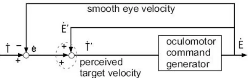
processing. From the theory of control point of view, it' s possible to estimate the target velocity, ˙T from sensory variables, by the sum of the retinal slip, ˙e and the eye velocity ˙E:

˙

T = ˙e + ˙E (1)

When the model estimate the target velocity, due to delays about the visual information processing, it will not receive the information about the retinal slip at the present time. The retinal slip carry information about the velocity of the target in past, i.e., ˙e(t − 4). So it can just estimate the target velocity at the time (t − 4). One of the most common solution is to employ a Kalmann lter for prediction. However, this model assumed prior knowledge of the tar-get dynamics and, thus, avoided to address how unknown tartar-get motion can be tracked accurately. S. Schaal and T. Shibata [1, 2] present a biologically motivated smooth pursuit controller that learns to predict the visual target ve-locity in head coordinates based on fast on-line statistical learning of the target dynamics. Their model consist in two subsystems: one is a target velocity pre-dictor, that predict the velocity of the target in the future ˙T (t + 4) and the other is an inverse model controller of the oculomotor system. The cascade of this two subsystems is inspired by an hypothesis based on neurophysiological studies: the higher visual cortex area generates the pursuit command which is sent to cerebellum where inverse model control is executed. For tracking a target having a simple linear dynamics such as a swinging pendulum, they employed an adapted version of Recursive Least Squares (RLS). The problem about this model is the initial response that is poor and the converging speed is slower than that in humans. To improve that performance is possible to use an appropriate anticipation in RLS. In this project, the idea is to include a memory block that recognize a specic velocity prole and gives the RLS appropriate parameters for a more accurate prediction. In general this memory block can be seen as an internal model that can help to predict the visual target velocity.

Figura 1: Classical Smooth Pursuit model based in a simple visual negative feedback controller.

predicted output. λ is a forgetting factor, discussed below. P (t) = 1 λ[P (t − 4) − P (t − 4)x(t)x(t)T_{P (t − 4)} λ + x(t)T_{P (t − 4)x(t)} ] (2) w(t) = w(t − 4) + P (t)x(t) λ + x(t)T_{P (t)x(t)}˙e(t + 1) (3) ˆ y(t) = w(t)Tx(t) (4) This strategy corresponds to training RLS on `fake' targets, i.e. y = ˆy(t) + ˙e. Initially, these fake targets are fairly distant from the true targets, such that RLS is actually trained on incorrect data. For this purpose, the model needs to forget data from early training, accomplished by the forgetting factor λ, which lies in the [0, 1] interval. For λ = 1, no forgetting takes place, while for smaller values, older values in the matrix P are exponentially forgotten. Essentially, the forgetting factor ensures that the prediction of RLS is only based on 1/(1 − λ) data points. This forgetting strategy also enables the predictor to be adaptive to the changes in the target dynamics. Another important element of Eq.(3) is that it explicitly shows the requirement for the time alignment of the predictor output and the error since the learning module cannot see ˙e(t + 1) at time t. Thus, all variables in Eq.(3) need to be delayed by one time step, which requires the storage of some variables for a short time in memory.

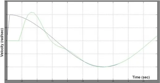
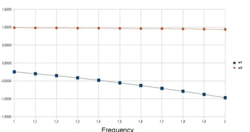
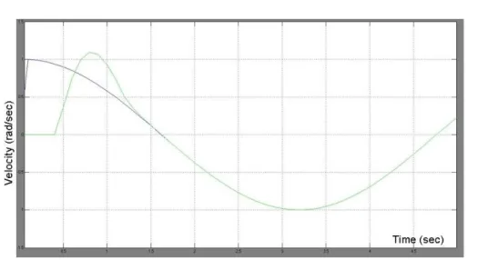
This model is simulated on Matlab-Simulink and the result are show in (Fig-ure 3) and (Fig(Fig-ure 4). The smooth pursuit are successfully accomplished in the case of the sinusoidal target motion. After about 5 seconds the model learn the target dynamics and the vector of regression parameters reachs the steady state (Figure 5). This converging speed is slower than that in humans, and if a second dynamics is presented at the model, it will need others 5 seconds to reach a new steady state, independentley if the second dynamics are already presented or not. Figure (6) shows that there is a direct relationship between frequency of the target dynamics and the nal weights of the model. It is possible to use such weights to correctly predicts the already seen target motion. In (Figure 7) and (Figure 8) the weights are set to the correct values after 1 second and the

Figure 3: Simulation result on Matlab Simulink for 1Hz sinusoidal target dy-namic. The gure shows the velocity of the target (blue line) and the output velocity (green line).

Figure 5: Vector of regression parameters.

Figure 6: Relationship between frequency of the target dynamics and the nal weights of the model.

Figure 7: Simulation result on Matlab Simulink for 1Hz sinusoidal target dy-namic with correct weights set after 1 second.

retinal slip just after reachs zero. This suggest that is possible storage the pre-viously acquired weights in to a memory block to improve the converging speed. From neurophysiological poin of view [3] the visual motion information follow the dorsal pathway and are elaborate by primary visual cortex, MT (middle temporal area) and MST ( medial superior temporal area). This area provides the sensory information to guide pursuit movements but may not be able to initiate them (Figure 9). The frontal eye eld, in the premotor cortex, is more important for initiating pursuit and it's also related with associative memory. Then, it's possible suppose that the brain keep motion information and use it to realize correct smooth pursuit.

In this project, Schaal's moodel has been modied to improve the perfor-mance on already seen target motions. A memory block (Figure 10) has been added to recognize target dynamics and it provides the correct weights values before the RLS algorithm.

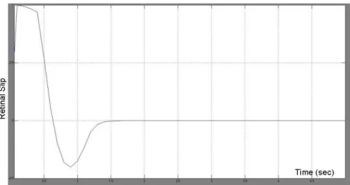
Figure 8: Retina slip with correct weights set after 1 second.

Figura 9: Pathways for smooth pursuit eye movements in primate.

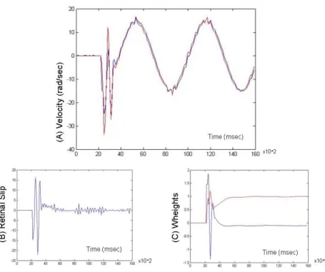
Figure 11: Robot Cub simulator result

Implementation and result

The modied model has been implemented on the iCub simulator that is able to simulate the external word phisical law and real robot respons. The robot correctly predicts (red line in Figure 11A) the target dynamics (blue line) in spite of the fact that the simulator is very dependent on PC performance and the target dynamic is not uid. The retinal slip reachs zero after about 5 seconds (Figure 11B) and the vector of regression parameters reachs the steady state (Figure 11C). Such weights values are stored in a Neural Network for future presentation of learned target dynamics.

Author: Davide Zambrano (Master student in Biomedical Engineering. Mail: d.zambrano@sssup.it );

Supervised: Cecilia Laschi (PhD Associate Professor of Biomedical Engi-neering Scuola Superiore Sant'Anna. Mail: cecilia@arts.sssup.it).