ENHANCED FEM-DBEM
APPROACH FOR FATIGUE
CRACK-GROWTH
SIMULATION
Venanzio Giannella
Unione Europea UNIVERSITÀ DEGLI STUDI DI SALERNO
FONDO SOCIALE EUROPEO
Programma Operativo Nazionale 2000/2006“Ricerca Scientifica, Sviluppo Tecnologico, Alta Formazione” Regioni dell’Obiettivo 1 – Misura III.4
“Formazione superiore ed universitaria”
Department of Industrial Engineering
Ph.D. Course in Mechanical Engineering
(XVI Cycle-New Series, XXX Cycle)
ENHANCED FEM-DBEM APPROACH FOR
FATIGUE CRACK-GROWTH SIMULATION
Supervisor
Ph.D. student
Prof. Roberto Guglielmo Citarella
Venanzio Giannella
Scientific Referee
Prof. Renato Esposito
Ph.D. Course Coordinator
List of publications
R. Citarella, V. Giannella, M. Lepore, DBEM crack propagation for nonlinear fracture problems, Frattura ed Integrità Strutturale, 34 (2015) 514-523; DOI: 10.3221/IGF-ESIS.34.57.
R. Citarella, V. Giannella, E. Vivo, M. Mazzeo, FEM-DBEM approach for crack propagation in a low pressure aeroengine turbine vane segment, Theoretical and Applied Fracture Mechanics, Volume 86, Part B, December 2016, Pages 143-152, DOI: 10.1016/j.tafmec.2016.05.004.
R. Citarella, V. Giannella, M. Lepore, G. Dhondt, Dual boundary element method and finite element method for mixed-mode crack propagation simulations in a cracked hollow shaft, DOI: 10.1111/ffe.12655.
V. Giannella, J. Fellinger, M. Perrella, R. Citarella, Fatigue life assessment in lateral support element of a magnet for nuclear fusion experiment “Wendelstein 7-X”, Engineering Fracture Mechanics, Volume 178, 1 June 2017, Pages 243-257, DOI: 10.1016/j.engfracmech.2017.04.033.
R.C. Wolf, V. Giannella, et alii., Major results from the first plasma campaign of the Wendelstein 7-X stellarator, DOI: 10.1088/1741-4326/aa770d.
V. Giannella, M. Perrella, R. Citarella, Efficient FEM-DBEM coupled approach for crack propagation simulations, Theoretical and Applied Fracture Mechanics, Volume 91, October 2017, Pages 76-85, DOI: 10.1016/j.tafmec.2017.04.003.
R. Citarella, V. Giannella, M. Lepore, J. Fellinger, FEM-DBEM approach to analyse crack scenarios in a baffle cooling pipe undergoing heat flux from the plasma, 2017, AIMS Journal 4(2):391-412, 2017, DOI: 10.3934/matersci.2017.2.391.
6
V. Giannella, R. Citarella, J. Fellinger, R. Esposito, LCF assessment on heat shield components of nuclear fusion experiment “Wendelstein 7-X” by critical plane criteria, Procedia Structural Integrity 8 (2018) 318-331.
I
Summary
Summary ... I List of figures ... III List of tables ... VI Abstract ... VII
Introduction ... 1
I General aspects ... 1
II Fracture Mechanics... 3
III Numerical analyses ... 5
IV Boundary Element Method (BEM) and Dual BEM ... 6
V Description of Thesis... 8
Chapter I FEM-DBEM approaches to Fracture Mechanics ... 11
I.1 Introduction ... 11
I.2 Superposition principle for Linear Elastic Fracture Mechanics ... 13
I.3 FEM-DBEM coupled approaches ... 14
I.4 Crack-growth criteria ... 16
I.4.1 SIF evaluation ... 16
I.4.2 Kink angle assessment ... 18
I.4.3 Crack-Growth Rate (CGR) assessment ... 20
I.4.4 Mixed-mode crack-growth ... 21
Chapter II FEM-DBEM benchmark ... 23
II.1 Introduction ... 23
II.2 Problem description ... 23
II.3 DBEM modelling ... 26
II
II.5 FEM-DBEM modelling ... 29
II.6 Results ... 31
II.7 Remarks ... 35
Chapter III Aeroengine turbine FEM-DBEM application ... 37
III.1 Introduction ... 37
III.2 Problem description ... 37
III.3 FEM modelling ... 38
III.4 Metallographic post-mortem investigation ... 40
III.5 DBEM submodelling approach ... 41
III.6 Results ... 45
III.7 Remarks ... 49
Chapter IV FEM-DBEM application on Wendelstein 7-X structure ... 51
IV.1 Introduction ... 51
IV.2 Problem description ... 51
IV.3 FEM modelling ... 56
IV.4 DBEM modelling ... 58
IV.5 Fatigue load spectra ... 61
IV.6 Results ... 63
IV.7 Remarks... 70
Conclusions ... 71
References ... 73
List of figures
Figure 1 Example of brittle fracture of a Liberty ship after splitting in two at
her outfitting dock; welded structure, rather than bolted, offered a continuous path to cracks to propagate throughout the entire structure (Parker, 1957) . 2
Figure 2 Example of fatigue crack-growth in a turbofan engine (Pratt &
Whitney JT8D) occurred during the take-off roll; a fan disk penetrated the left aft fuselage determining two fatalities (www.wikipedia.it). ... 3
Figure 3 (a) Traditional designing philosophy vs. (b) Damage Tolerance
design philosophy. ... 4
Figure 4 Example of a 2D model via (a) FEM and (b) BEM. ... 6 Figure 5 Example of (a) FEM and (b) BEM models of a reinforced curved
fuselage panel (Aliabadi, 2002) ... 6
Figure I. 1 Example of a (a) FEM and a (b) DBEM submodelling of a gear
tooth with a crack (2D problem). ... 12
Figure I. 2 Superposition principle applied to a fracture problem; 𝜎0 is the
pre-existing stress field generated by the applied prescribed conditions, etc. ... 13
Figure I. 3 Different approaches for the selection of the DBEM submodel
loading conditions for a gear tooth with a crack: (a) Fixed Displacement (FD); (b) Fixed Load (FL); (c) Loaded Crack (LC). ... 15
Figure I. 4 Closed path around crack tip (Wilson, 1976). ... 17 Figure I. 5 Schematic plot of the typical 𝑑𝑎𝑑𝑁 vs. ∆𝐾 relationship; the Paris
law is calibrated to model the linear part of the graph. ... 20
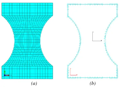
Figure II. 1 Drawings of the (a) shaft with highlight of the crack and fillet
radii, (b) hub with the dotted red line representing the loading application zone. ... 24
Figure II. 2 Considered load cases: (a) ‘‘coupled”, (b) ‘‘shear” and (c)
‘‘torque”. ... 25
Figure II. 3 DBEM uncracked model with close‐up of the remeshed area surrounding the crack insertion point and details of the initial crack geometry with J‐paths along the crack front (purple) for the J‐integral computation. ... 27
Figure II. 4 ZENCRACK (ZC)/ABAQUS uncracked model with highlight on
IV
Figure II. 5 CRACKTRACER3D (CT3D)/CalculiX uncracked model with
the subsequent cracked mesh and details of the crack. ... 29
Figure II. 6 (a) FEM and DBEM submodel used for the FEM-DBEM
approach; (b) DBEM submodel after that the crack has been inserted and loaded. ... 31
Figure II. 7 SIFs calculated by the considered methodologies for load
cases: (a) coupled, (b) shear and (c) torque; X-axis is the normalised
abscissa drawn along crack front... 32
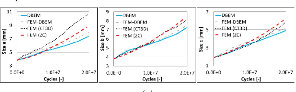
Figure II. 8 Crack size definitions. ... 34 Figure II. 9 Plots of crack sizes vs. total fatigue cycles for the load cases of:
(a) coupled; (b) shear; (c) torque. ... 35
Figure III. 1 Material properties vs. temperature for the considered
superalloy: Young’s modulus (a), thermal expansion coefficient (b) and Poisson’s ratio (c). ... 39
Figure III. 2 FEM model: (a) thermal scenario and (b) cyclic symmetry
boundary conditions (highlighted in green). ... 40
Figure III. 3 Tangential displacements (a) and max principal stresses (b) on
the statoric segment. ... 40
Figure III. 4 Segment affected by fatigue failure: (a) damaged airfoil with
highlight (yellow arrows) of the undesired double radius on the trailing edge; (b) estimated initial crack front (red line). ... 41
Figure III. 5 (a) Realistic engine mission profile and (b) its simplified profile
adopted in this work. ... 42
Figure III. 6 Considered loading strategies for DBEM analyses: (a) LC and
(b) FD; model for LC comprises the self-equilibrated load on the crack face elements and few constraints to prevent rigid body motion; model for FD comprises temperature on all the elements and displacement field on all the cut surface elements. ... 44
Figure III. 7 Max principal stresses before crack introduction on the two
DBEM submodels used for FD approach; highlight of the crack insertion position. ... 44
Figure III. 8 Von Mises stresses [psi] for the initial cracked FD (a) and LC
(b) models, with close-up of the cracked area (cutting sphere radius R = 1 in.). ... 46
Figure III. 9 Different meshes on the crack face, as used for the convergence
study. ... 47
Figure III. 10 Different meshes on the crack face, as used for the convergence
study between (a) LC and (b) FD methods; X axis is the normalised abscissa drawn along the crack front. ... 47
Figure III. 11 Comparison on crack sizes vs. cycles plots for small and large
submodels and both the methodologies: (a) LC and (b) FD. ... 48
Figure IV. 1 (a) Modular-type stellarator Wendelstein 7-X; (b) Hot plasma
V
the magnet system of W7-X; (d) W7-X magnet system: FEM detail of a half module with the LSEs; highlights on the investigated LSE-05. ... 54
Figure IV. 2 LSE-05: real component with highlight of discovered surface
cracks; continuous circle (red line) surrounding the most critical (and modelled) crack. ... 55
Figure IV. 3 Von Mises stresses [Pa], related to the load case with EM field
of 3 T “HJ”, on the: (a) FEM global model, (b) first FEM LSE-05 submodel, (c) furtherly reduced FEM submodel. Red arrow in (a) pointing out the submodelled LSE-05 in (b). Dashed red square in (b) representing the area that has been furtherly refined in (c). ... 57
Figure IV. 4 (a) FEM submodel and (b) DBEM uncracked submodel (the red
dot is the crack insertion point), obtained by a Boolean subtraction with a sphere of radius 0.11 m. ... 59
Figure IV. 5 DBEM cracked submodel with highlight of the different modelled
zones. ... 59
Figure IV. 6 DBEM submodel loaded with different BCs: either (a)
displacements (FD) or (c) tractions (FL) applied on cut surfaces; (b) tractions applied on the crack faces (LC). ... 60
Figure IV. 7 Schematic loading history due to EM forces. ... 62 Figure IV. 8 (a) DBEM crack (deformed shape) with the applied tractions (in
orange) for the LC approach; (b) crack sizes definition with J-paths along crack front (in purple). ... 64
Figure IV. 9 (a) Von Mises stress scenario for LC approach; initial crack
configuration and load case iii; (b) close up of the von Mises stress scenario in the crack surroundings for LC approach; initial crack configuration and load case iii. ... 64
Figure IV. 10 Von Mises stress scenario from FD/FL approach; initial crack
configuration and load case iii... 65
Figure IV. 11 SIF values along the crack front for FD, FL and LC approaches
for all the load cases from i to v. ... 66
Figure IV. 12 Final crack shape; traction BCs (in orange) applied on the
crack face elements for LC approach; dashed black line representing the initial edge of the inserted crack. ... 66
Figure IV. 13 Crack sizes vs. number of cycles under (a) daily and (b) weekly
load spectra. ... 68
Figure IV. 14 Equivalent SIFs vs. number of cycles under (a) daily and (b)
List of tables
Table II. 1 Main material data for mechanical and fracture analyses. ... 26
Table II. 2 Runtime for the entire propagation for the coupled load case for the various adopted approaches. ... 35
Table III. 1 Mechanical, thermal and fatigue properties at the sub-model average temperature. ... 43
Table III. 2 Runtimes compared for FD and LC approaches. ... 49
Table IV. 1 Mechanical properties at temperature of 4 K. ... 59
Table IV. 2 Fatigue elementary block corresponding to 10 working days with the daily spectrum (12.1 cycles per working day). ... 62
Table IV. 3 Fatigue elementary block corresponding to 50 working days with the weekly spectrum (5.42 cycles per working day). ... 62
Table IV. 4 Paris’ law parameters at temperature of 4 K. ... 63
Table IV. 5 Forman’s law parameters at temperature of 4 K. ... 63
Abstract
To comply with fatigue life requirements, it is often necessary to carry out fracture mechanics assessments of structural components undergoing cyclic loadings. Fatigue growth analysis of cracks is one of the most important aspects of the structural integrity prediction for components (bars, wires, bolts, shafts, etc.) in presence of initial or accumulated in‐ service damage. Stresses and strains due to mechanical as well as thermal, electromagnetical, etc., loading conditions are typical for the components of engineering structures. The problem of residual fatigue life prediction of such type of structural elements is complex, and a closed form solution is usually not available because the applied loads not rarely lead to mixed-mode conditions.
Frequently, engineering structures are modelled by using the Finite Element Method (FEM) due to the availability of many well‐ known commercial packages, a widespread use of the method and its well-known flexibility when dealing with complex structures. However, modelling crack-growth with FEM involves complex remeshing processes as the crack propagates, especially when mixed‐ mode conditions occur. Hence, extended FEMs (XFEMs) and meshless methods have been widely and successfully applied to crack propagation analyses in the last years. These techniques allow a mesh‐ independent crack representation, and remeshing is not even required to model the crack growth. The drawbacks of such mesh independency consist of high complexity of the finite elements, of material law formulation and solver algorithm.
On the other hand, the Dual Boundary Element Method (DBEM) both simplifies the meshing processes and accurately characterizes the singular stress fields at the crack tips (linear assumption must be verified). Furthermore, it can be easily used in combination with FEM and, such a combination between DBEM and FEM, allows to simulate fracture problems leveraging on the high accuracy of DBEM when working on fracture, and on the versatility of FEM when working on complex structural problems. Generally, FEM is used to tackle the global complex structural problem, assessing the fields of displacements, strains and stresses; subsequently, such fields are used to obtain the boundary conditions to apply on a DBEM submodel that bounds the region in which the crack is present. In this way, the
Abstract
VIII
fracture problem is solved in the DBEM environment allowing to take advantage of its inherently simpler remeshing process. Such FEM-DBEM “classical” approach has been previously implemented under fixed either displacements or tractions boundary conditions applied on the DBEM submodel cut surfaces, without updating of their values during the propagation. Such boundary conditions are consequently assumed to be insensitive to the submodel stiffness variation due to the crack-growth, with the consequent introduction of an element of approximation that limits the accuracy of results. In case of traction boundary conditions the approach provides conservative results in terms of residual life cycles, whereas, non-conservative results are obtained in case of fixed displacements boundary conditions. Interestingly, the here proposed alternative approach provides results comprised between the upper and lower bounds given by such two classical approaches.
This work presents an enhanced FEM-DBEM submodelling approach to simulate fracture problems through the adoption of the principle of linear superposition. Theoretical background can be found in the literature, where the J-integral for a thermal-stress crack problem was retrieved by a simple application of a load distribution on the crack faces (as provided by the uncracked problem solution) instead of the application of the inherent displacement or traction condition on the model boundary. This idea has been here widely extended to more complex analyses allowing to solve fracture problems with very high accuracy by means of relatively simple DBEM stress analyses, even when the global analyses present thermal loads, contacts, friction, electromagnetic fields, etc. As a matter of fact, all the complexities are tackled by a global FEM analysis on the uncracked domain, whereas, the objectives of correctly predicting the whole crack-growth are completely demanded to the DBEM.
The methodology has been validated comparing the results with those provided by different numerical approaches, like the well-established classical FEM-DBEM approaches or fully FEM based approaches, as available from literature.
Then, some industrial applications have been analysed by means of this new methodology showing that the procedure can also handle problems of higher complexity leading to an accuracy on the results that, in some cases, could not even be obtained with the classical approaches.
Introduction
I General aspects
Starting from the industrial revolution around the late 18th century, metals were seen as the most successful and all-purpose construction materials. They were mainly chosen for their high strength to weight ratio, workability and availability. Today many buildings, ships, aircrafts and many other engineering structures are still largely built out of metals. Unfortunately, many of this metal structures did not live as per their expectations and many of them collapsed catastrophically under regular service conditions. Furthermore, most of these structural failures occurred very often without adequate warnings and, as a result, many human lives have been lost. The cause of such catastrophic failures (Figs. 1-2) could often be attributed to a combination of material deficiencies in the form of pre-existing flaws in the material, poor designs, in-service damages, etc.
To ensure safety, current specific standards require routine periodic checks for detecting possible cracks. Then, cracked components have to be monitored and, if necessary, replaced or repaired before they become critical. Improvement at the design stage, where high stress concentrations in the structure should be avoided, better production methods as well as enhancement of material properties have all helped to minimize the criticalities and consequently have reduced the number of failures. However, total elimination of cracks is not only impractical but also impossible because cracks often develop well below the material yield strength. To further mitigate fracture failures, the so called design philosophy “Damage
Tolerance” has been introduced in recent years at the design stage where
engineers have to anticipate the likelihood of cracks in the structural components.
As structures are becoming more complex, the need for an accurate and reliable assessment of the structural safety has become mandatory. A simple arbitrary safety factor is no longer an acceptable safety margin, nor is it justified in terms of economy and efficiency. The need for reliable engineering decisions has prompted the development of a methodology to compensate for the inadequacies of conventional design concepts. Although the conventional
FEM-DBEM approaches to Fracture Mechanics
2
design criteria based on the material strength can be adequate for many engineering structures, they are insufficient when there is the likelihood of native and/or accumulated in-service defects.
In this framework, Fracture Mechanics is often used to provide the necessary additional safety checks, understandings of the fracture processes and, even more important, obtaining reliable predictions on the residual strength of the structure.
Figure 1 Example of brittle fracture of a Liberty ship after splitting in two at
her outfitting dock; welded structure, rather than bolted, offered a continuous path to cracks to propagate throughout the entire structure (Parker, 1957)
Chapter I
3 Figure 2 Example of fatigue crack-growth in a turbofan engine (Pratt &
Whitney JT8D) occurred during the take-off roll; a fan disk penetrated the left aft fuselage determining two fatalities (www.wikipedia.it).
II Fracture Mechanics
Beginning with catastrophic failures of railway components through to serious failures of many Liberty ships during World War II, there are many grim examples of the debilitating effects of flaws on the material strength. It has also emerged during this century that the conventional criteria of tensile strength, yield strength and buckling stress are not always sufficient to guarantee the overall component integrity. This has been especially evident with the introduction of high strength materials, which are correspondingly low in crack resistance. Furthermore, structural engineers are continuously struggling to reduce safety margins between the stresses expected during the working conditions and the strength of materials. All of these conditions have spurred the development of Fracture Mechanics, especially in the last two decades, to enable dedicated analyses of components with crack-like defects. The discipline of Fracture Mechanics (Anderson, 1991) enables the prediction of crack behaviour to be quantitatively achieved. Namely, Fracture Mechanics has been used to predict the crack size below which no crack-growth would occur, or, the crack size at which a component would fail given a certain applied fatigue load. In between these two limits, Fracture Mechanics allows to estimate the rate of crack-growth and then allows to predict the life of a cracked component under fatigue loading. This allowed going beyond the
FEM-DBEM approaches to Fracture Mechanics
4
traditional design standpoint (Fig. 3a), in which only the requested loads were compared with the material strength, to the concept of Damage Tolerance design process (Fig. 3b), in which also the presence of defects has to be taken into account in the process. Fracture Mechanics analyses are then carried out to obtain the component life with a pre-defined initial flaw size and the expected fatigue loading conditions. Such life must exceed the operational life needed for a given structure otherwise the component geometry has to be redesigned or, otherwise, the loading revised. Inspection intervals can then be set to ensure that crack-growth is less than that predicted or, if not, the component has to be either repaired or replaced.
Fracture Mechanics is based on continuum mechanics concepts, which express given relationships between the stress and displacement fields at the crack tips. Under the small strains and linear elastic assumptions, it is found that the stress fields in close vicinity of the crack tip are inversely proportional to the square root of the distance from the tip itself. The constant of proportionality is the Stress Intensity Factor (SIF), which defines the intensity of the singular stress field at the crack tip. It is also found from experiments that failure occurs when, under static load conditions, the SIF reaches the critical value for the material and, therefore, an accurate determination of SIF is of extreme importance for the consequent estimate of the structural integrity. Moreover, when dealing with fatigue loading conditions, the precise SIF evaluation is of utmost importance for the Crack-Growth Rate (CGR) prediction and eventually for the residual fatigue life assessment.
(a)
(b)
Figure 3 (a) Traditional designing philosophy vs. (b) Damage Tolerance
Chapter I
5
III Numerical analyses
Obviously, analytical techniques cannot tackle all the complexities encountered in all the engineering structural components. Therefore, numerical techniques have been widely developed in recent years, encouraged especially by the enormous advances in the computer technology.
Nowadays, FEM is the most widely used in the engineering designing process thanks to its advantages when simulating several physical phenomena. The method is widely used in the industries since it is able to face problems involving: contacts, frictions, mechanical, thermal and electromagnetical loads, complex constitutive law formulations, impacts, etc. There are various ways of tackling Fracture Mechanics by FEM and, definitely, FEM has been efficiently used along the years in several applications. However, it typically needs long model preparation times. In addition, especially when the crack propagates generating complex three-dimensional shapes, the method is not anymore suitable to simulate the fracture process due to distortion of elements nearby the crack, too long runtimes, etc.
The Boundary Element Method, together with its enhanced version Dual BEM, can circumvent the limitations of FEM on complex crack propagation problems (Aliabadi, 1991, 1992; Brebbia, 1984, 1989). This method is based on the solution of integral equations, that govern elasticity and potential theory. Such a method works with the discretization of the only boundary into elements over which the product of shape functions, Green’s functions and element Jacobians, are numerically integrated. This results in higher accuracy particularly when the domain to be discretised contains regions of high stress gradients (such as cracks) which would necessitate a considerable concentration of FEM elements and nodes. Hence, DBEM is particularly suited to Fracture Mechanics analyses due to the accuracy of the results and the inherently better and simpler remeshing process as the crack increases in size.
Since only the boundaries of the domain are discretised, the dimensionality of the domain is reduced by one, reducing then the size of the mathematical problem to handle (Fig. 4). However, the system matrix is unsymmetric and fully populated and therefore, generally, it takes longer runtimes than those needed by FEM to obtain the solution. More generally, considering the computational power nowadays available, DBEM remains more attractive, when working on fracture, comparing the preprocessing efforts of the two aforesaid numerical methods (Fig. 5).
FEM-DBEM approaches to Fracture Mechanics
6
(a) (b)
Figure 4 Example of a 2D model via (a) FEM and (b) BEM.
(a)
(b)
Figure 5 Example of (a) FEM and (b) BEM models of a reinforced curved
fuselage panel (Aliabadi, 2002)
IV Boundary Element Method (BEM) and Dual BEM
BEM has become established as an effective alternative to FEM in several important areas of engineering analysis. Although the BEM, also known as the Boundary Integral Equation (BIE) method, is a relatively new technique for engineering analysis the fundamentals can be traced back to classical mathematical formulations by Fredholm (Fredholm, 1903) and Mikhlin (Mikhlin, 1957) in potential theory and Betti (Betti, 1872), Somigliana (Somigliana, 1886) and Kupradze (Kupradze, 1965) in elasticity.
Chapter I
7 Basically, the aim is to transform the governing differential equations defined in the domain into an integral equation which applies only to the boundary of the domain. Such an integral equation depends on the availability of:
a fundamental solution to the governing differential equation for a point force;
a reciprocal relationship (such as Green’s theorem; Green, 1828) between two functions which are continuous and possess continuous first derivatives.
The choice of the unknowns has led to two formulations of the boundary integral equations: the direct method, where the unknowns are the actual physical variables in the problem, such as displacement or traction in elasticity; the indirect method that historically precedes the previous one. In the latter approach, the unknowns are fictitious density functions which have no physical significance but from which the physical unknowns can be obtained by postprocess.
In order to obtain the boundary integral equations, a powerful and general technique is the weighted residual method of Brebbia (1977, 1978) where the error residual is minimized. Jeng and Wexler used a variational formulation similar to that of the finite elements and Cruse and Rizzo (Rizzo, 1967; Cruse, 1969) employed Betti’s reciprocal work theorem.
For many years, the potential of boundary integral equations was not realized due to the difficulty of attaining analytical solutions to the integral equations for practical problems and due its essentially mathematical origins. However, research into the numerical solution of boundary integral equations was prompted by the advent of high speed computing. As computers grew in power and storage, the amenable problems became more complex. This resulted in the numerical method now known as BEM. Brebbia demonstrated that not only it is related to FEM but that both methods can be derived from the same variational equation (Brebbia, 1978).
In the BEM, the boundary integral equations are discretized so that numerical integration is carried out over a small part (element) of the boundary, over which the variation of the boundary variables is expected to be small. Variation over an element is handled in a similar way to that of the finite elements. For example, considering an elastostatic problem, the variation of displacements and tractions over an element is approximated by opportune shape functions related to nodal values of displacements and tractions respectively. Each collocation node will yield either two or three boundary integral equations depending on the dimensionality of the problem. By moving this collocation point to each node in the model, a system of equations is built up in which the displacement at each point is related to the displacement and tractions on all points on the boundary. The resulting matrices are therefore fully populated and unsymmetric. This is in contrast to
FEM-DBEM approaches to Fracture Mechanics
8
the sparse and banded FEM system matrix which, however, are generally much larger for an equivalent problem.
It is worth noting that only the boundary of the model needs to be discretized as the governing (elastostatic) differential equations are satisfied in the interior region. The data preparation is carried out only for the boundary, avoiding the domain discretization used by the FEM. This results in a method that is particularly suited to Fracture Mechanics analyses due to the accuracy of the results both on the surface and at selected interior points.
The introduction of isoparametric variation over the boundary elements by Lachat and Lachat & Watson (Lachat, 1975, 1976) provided a further possibility to the BEM to fulfil its potential of high accuracy and efficiency. Quadratic variation of geometry was used over the elements and linear, isoparametric quadratic and cubic variation of the unknown displacement and traction were catered for. This enables the BEM to be more economical than FEM for certain types of problems, although FEM will be more appropriate for others. Anyway, both techniques should be made available to engineers. The adopted DBEM approach (Portela, 1990, 1993; Apicella, 1994; Mi, 1994; Fedelinsky, 1994) is a BEM enriched with special discontinuous elements appropriate to consider nodes and faces of the crack topologically coincident. The three-dimensional domain boundary is discretized into either 4, 8 or 9 noded quadrilateral elements, or 3 or 6 noded triangular elements. The boundary integral equations here adopted apply to a homogeneous isotropic domain and the linear elastic assumption must also be held. As aforesaid, with DBEM, only the crack faces and the other boundaries are discretized. Traction boundary integral equations are used for one crack face and displacement boundary integral equations are used for the second crack face and the remaining boundaries. So doing, being the traction and displacement equations independent, the system coefficient matrix turns out to be non-singular and, therefore, the solution can be retrieved.
V Description of Thesis
After an introduction, in chapter I it has been discussed on how to couple the FEM and DBEM methods to work out general Fracture Mechanics problems. At first, the need to adopt a submodelling strategy when solving fracture problems on large structures has been introduced. Then, it has been argued on how to implement such a submodelling technique by using the FEM and DBEM methods. Three FEM-DBEM submodelling approaches have been presented and the advantages of using the “Loaded Crack” (LC) approach highlighted. By means of such an approach, based on loading only the DBEM crack faces, the most accurate results in terms of SIFs, CGRs and crack paths can be obtained.
Chapter I
9 In chapter II, it has been shown how the LC approach has been applied on a shaft-hub coupling that undergoes different loading conditions. The results have been compared with those obtained by leveraging on a pure DBEM approach and with two different FEM codes showing a very sound agreement. A first industrial application of the LC approach has been presented in chapter III. It consisted in a crack propagation simulation in an airfoil of a statoric segment of a GE-Aviation aeroengine. The LC approach turned out to be more efficient in terms of computational effort and more accurate in terms of fatigue life estimate, when compared with a classical FEM-DBEM approach.
In chapter IV, it has been presented a further industrial application of the three FEM-DBEM approaches on a component of the magnetic cage of the nuclear fusion experiment “Wendelstein 7-X”. The residual fatigue life has been estimated with all the approaches and the results compared and discussed. Again, the LC approach turned out to be more accurate than the classical approaches.
All the DBEM and FEM-DBEM calculations shown in chapters II-IV were executed on a workstation with the following general configuration: motherboard MSI X99S SLI Plus, CPU Intel i7-5820K with 15MB L3 cache, RAM 8x 8GB HyperX Fury DDR4, SSD Samsung 850 2x 250GB and Windows 7 Professional 64bit SP1.
Chapter I
FEM-DBEM approaches to
Fracture Mechanics
I.1 Introduction
FEM and BEM are effective tools for the numerical analysis of many physical problems described with a set of partial differential equations and frequently impossible to solve analytically.
With regard to particular aspects, the two methodologies are complementary, each of them having preferential applications. Namely, FEM is well suited for complex analyses containing nonlinearities, massive meshes, contacts, anisotropic materials, etc., whereas BEM and in particular DBEM (Dual BEM) (Aliabadi, 1992a, 1992b; Portela, 1990; Fedelinsky, 1994) are generally preferred in the Linear Elastic Fracture Mechanics (LEFM) context, to get accurate SIFs (Stress Intensity Factors) evaluations and automatic crack propagations (Apicella, 1994).
Although the fracture phenomenon plays essentially a local effect if compared to the overall structure (i.e. the singular fields at crack tip, the possible crack propagation, etc.), it cannot be overlooked. An initial small crack, after it propagates throughout the structure, can lead to the failure of the entire structure as taught by well-known past catastrophic failures (Figs. I.1, I.2). Numerical analysis can be used as a tool to better understand how fracture phenomena affect structures in order to prevent catastrophic failures. When one or more cracks have to be numerically modelled in large structures, a submodelling approach is generally mandatory in order to make the approach amenable from a computational standpoint and also to reduce the size of the models to handle. Especially when such structures are modelled by FEM, this submodelling approach plays an even more important role since the cracks would need very fine meshes in their surroundings with the consequent sharp increase of runtimes. The DBEM would be more attractive in this context thanks to its intrinsic nature of meshing only the model boundaries and one or multiple cracks can be modelled more easily than by
FEM-DBEM approaches to Fracture Mechanics
12
FEM. However, the inherent restrictions of the DBEM do not allow tackling all the industrial problems as a standalone tool.
As a consequence, great research efforts have been aimed along the years at improving the synergetic usage of the two previously mentioned methodologies (McNamee), in order to exploit the FEM versatility in combination with the intrinsic better features of DBEM for modelling fracture. This work presents three approaches that allow to adopt a submodelling approach (Fig. I.1), to strongly reduce the runtimes, and specifically a FEM-DBEM coupling, to get the highest accuracy on results by benefiting from both the diverse advantages of FEM and DBEM.
Two approaches are based on replicating the FEM global fields in a DBEM local submodel, where the fracture problem is worked out. These two approaches provide an upper and a lower bound in terms of residual fatigue life estimate. We will see how, the third approach, based on the application of the superposition principle to Fracture Mechanics problems, provides the most efficient and accurate fracture assessment.
Figure I. 1 Example of a (a) FEM and a (b) DBEM submodelling of a gear
Chapter I
13
I.2 Superposition principle for Linear Elastic Fracture Mechanics
Wilson (Wilson, 1979) showed that the SIFs for a crack in a 2D thermal-stress problem could be calculated by means of a simpler thermal-stress analysis in which no external loads were applied but just tractions on the crack faces. This was possible leveraging on the principle of linear superposition applied to a Fracture Mechanics problem, as explained in the followings.
Figure I. 2 Superposition principle applied to a fracture problem; 𝜎0 is the
pre-existing stress field generated by the applied prescribed conditions, etc.
Extending the Wilson’s example to the most general crack problem schematically shown in Fig. I.2, the superposition principle can be then applied as explained in the following steps:
from an original uncracked domain (A), a crack can be opened (B) and loaded with tractions equal to those calculated over the same dashed line in (A);
the new configuration (B), perfectly equivalent to (A), can then be transformed by using the superposition principle, splitting the boundary conditions as in (C) and (D);
(C = C’) represents the real fracture problem to be solved, whereas (D), after the tractions sign inversion, turns in an equivalent problem (D’) that will be effectively tackled.
FEM-DBEM approaches to Fracture Mechanics
14
In conclusion, using boundary conditions retrieved from the considered uncracked problem (A), a purely stress crack problem (D’) can be considered for the fracture assessment; in such equivalent problem, the crack faces undergo tractions equal in magnitude but opposite in sign to those calculated over the same (dashed) crack line in (A). In other words, SIFs for case (C’) are equal to those calculated for the simpler problem (D’). In final, the use of the superposition principle enables a faster convergence for the simpler DBEM pure stress analyses, in comparison with that provided by the more traditional FEM-DBEM approaches (those with transfer of displacement or traction boundary conditions on the submodel cut surfaces), with consequent reduction of computational burden.
I.3 FEM-DBEM coupled approaches
Considering the different FEM and DBEM capabilities, the most promising idea would be to use FEM to calculate the global displacement-strain-stress fields and to adopt such results to solve the local fracture problem by means of DBEM.
Here, two FEM-DBEM approaches are presented and, by considering the superposition principle explained in §I.2, a third one is proposed. The three approaches can be schematically explained by means of Fig. I.3. With reference to cases (b) and (c) in Fig. I.3, all the rigid body degrees of freedom have to be eliminated and this can done, as instance, by applying springs of negligible stiffness on few elements.
Basically, all the approaches are based on the submodelling technique in order to strongly reduce the computational efforts. The basic assumption is that the analysed fracture phenomena do not introduce a significant perturbation on the overall fields far from the crack area, so that, there is no need to explicitly model the entire structure for the fracture assessment.
A DBEM submodel can be then extracted by a Boolean operation of subtraction between the FEM model and a user defined cutting domain, providing, in the DBEM environment, a smaller model that surrounds the crack insertion area with just a surface mesh at its boundaries.
After the DBEM submodel extraction, a crack is inserted in the submodel and a remeshing, which typically involves just the crack surroundings, is realised. Subsequently, such DBEM cracked submodel is loaded with apposite boundary conditions in order to compute SIFs representative of those occurring in the real cracked component. Then, when requested, the crack propagation can be simulated by increasing step-by-step the crack dimensions, with the ith crack kinking and growth rate evaluated as a function of the SIFs
evaluated for the (i-1)th geometry. Moreover, for fatigue crack propagation simulations, one or more load cases are used to assemble the needed fatigue load spectra representative of the loads occurring during the real operation of
Chapter I
15 the components. Also, it has to be guaranteed that the crack tips remain adequately far from the cut surface boundaries over which displacements or traction were imposed.
Figure I. 3 Different approaches for the selection of the DBEM submodel
loading conditions for a gear tooth with a crack: (a) Fixed Displacement (FD); (b) Fixed Load (FL); (c) Loaded Crack (LC).
The DBEM submodel loading process can follow one of the three different previously mentioned approaches (example in Fig. I.3) explained in the following:
Fixed Displacement (FD) approach: the DBEM volume cut surfaces are loaded with displacement boundary conditions; Fixed Load (FL) approach: the DBEM volume cut surfaces are
loaded with traction boundary conditions;
Loaded Crack (LC) approach: the DBEM crack faces are loaded with traction boundary conditions.
In detail, two kind of inaccuracies unavoidably arise when using both FD or FL approaches. Firstly, such two approaches use boundary conditions that applied to a cracked model come from an uncracked global model. Secondly, boundary conditions are kept as fixed during the crack propagation simulation and therefore they are considered as insensitive to the continuously decreasing DBEM submodel stiffness induced by the growing crack. Both inaccuracies could be overcome by using a larger submodel but this would affect the runtimes without even completely eliminate such drawbacks. Anyway, the FD approach has been satisfactorily implemented in the past as in some works available in the literature (Citarella, 2013, 2014).
On the contrary, the LC approach allows to inherently consider step-by-step updated boundary conditions, since additional loading is provided on the crack extension area at each step of the incremental crack-growth simulation. In addition, the SIFs are rigorously calculated even by using boundary conditions that are coming from an uncracked model, as dictated by the superposition principle (§I.2). Moreover, there is no need to replicate the global FEM fields in the DBEM submodel and this widen the range of
FEM-DBEM approaches to Fracture Mechanics
16
amenable applications, namely more complex analyses can be restricted solely to FEM approach.
For these reasons, in the following it is shown that the LC approach represents the most enhanced strategy to couple FEM and DBEM, providing results with the highest accuracy in terms of SIF assessment and therefore also in terms of residual fatigue life estimate and crack path assessment. Such an approach is proposed in the current work by means of a FEM-DBEM submodelling strategy but, however, it can clearly be also applicable to FEM-FEM submodelling strategies or equivalents. It is worth noting that, for embedded cracks far enough from the external boundaries (e.g. voids, internal cracks), it would be possible to consider the cracks as in an infinite body so the DBEM boundary would be just the loaded crack faces and the corresponding mathematical problem notably reduced.
Besides the submodel loading conditions, in order to predict a Linear Elastic Fracture Mechanics (LEFM) incremental crack-growth, three basic criteria are required for the separate phases of: SIF evaluation, kink angle prediction and Crack-Growth Rate (CGR) assessment. The criteria that have been used in the current work are described in the followings together with some references about the most widely accepted ones.
I.4 Crack-growth criteria
A crack-growth simulation is typically worked out by means of an incremental crack-extension analysis in which the three distinct phases of SIF evaluation, kink angle prediction and CGR assessment are basically repeated until either a requested crack size or a critical K value is reached. Namely, for each crack extension, the SIFs are calculated and used to predict both the direction of the growth and the corresponding fatigue cycles. Various criteria have been proposed along the years and those adopted in this work are described in the followings.
I.4.1 SIF evaluation
There are several approaches to calculate SIFs such as: crack tip opening displacement (CTOD) approach (Citarella, 2010), crack tip stress field approach (Dhondt, 2014) and SIF extraction method from J-integral (Citarella, 2010). The J-integral, being an energy approach, has the advantage that elaborate representation of the crack tip singular fields is not necessary. This is due to the relatively small contribution that the crack tip fields make to the total J (i.e. strain energy) of the body. Therefore, in the present work, the SIFs are extracted from the J-integral calculation by leveraging on the method illustrated in the following.
Chapter I
17
𝐽 = ∫ (Wn𝑆 1− tj𝑢j,1)dS (I.1)
where 𝑆 is an arbitrary closed contour, oriented in the anti-clockwise direction, starting from the lower crack surface to the upper one and incorporating the crack tip, 𝑑𝑆 is an element of the contour 𝑆, 𝑊 is the strain energy per unit volume, n1 is the component in the x1 direction of the outward
normal to the path 𝑆, and tj(= σijnj) and uj,1 are the components of the interior tractions and strains, respectively.
J-integral can be related to a combination of the values of K𝐼 and K𝐼𝐼.
Ishikawa, Kitagawa and Okamura (Ishikawa, 1980) suggested a simple procedure for doing so and Aliabadi (Aliabadi, 1990) demonstrated that it can be implemented in the DBEM in a straightforward manner.
The application of the J-integral to 3D crack problems was presented by Rigby and Aliabadi (Rigby, 1993, 1998) and Huber and Kuhn (Huber, 1993). The application of the 3D J-integral to thermoelastic crack problems can be found in dell’Erba and Aliabadi (dell’Erba, 2000).
The J-integral for 3D is defined as 𝐽 = ∫ (Wn1− 𝜎ij 𝜕𝑢𝑖 𝜕𝑥1𝑛j) dΓ Γ𝜌 = = ∫ (Wn1− 𝜎ij𝜕𝑢𝑖 𝜕𝑥1𝑛j) dΓ 𝐶+𝜔 − ∫ 𝜕 𝜕𝑥3(𝜎𝑖3 𝜕𝑢𝑖 𝜕𝑥1) dΩ Ω(𝐶) (I.2)
where Γ𝜌 is a contour identical to C𝜌 but proceeding in an anti-clockwise direction (Fig. I.4). The integral J is defined in the plane x3= 0 for any
position on the crack front. Considering a traction free crack, the contour integral over the crack faces 𝜔 is zero, instead, with loaded crack faces, as for the LC approach here presented, the contribution of ∫ −𝜎ij𝜕𝑥𝜕𝑢𝑖
1𝑛jdω
𝜔 has to
be added.
FEM-DBEM approaches to Fracture Mechanics
18
For mixed-mode 3D problems, the J-integral is related to the three basic fracture modes through the components JI, JII and JIII:
J = JI+ JII+ JIII (I.3)
Rigby and Aliabadi (Rigby, 1998) presented a decomposition method through which the integrals JI, JII and JIII in elastic problems can be calculated
directly from J. Firstly, J was divided into two components:
J = JS+ J𝐴𝑆 (I.4)
J𝑆 and JAS are obtained from symmetric and anti-symmetric elastic fields
around the crack plane, respectively. As the mode I elastic fields are symmetric to the crack plane, the following relationship holds:
JS= J𝐼 and JAS= J𝐼𝐼+ J𝐼𝐼𝐼 (I.5)
JII and JIII integrals can be calculated from J𝐴𝑆 by making an additional
analysis on the anti-symmetric fields. Then, when J-integral is calculated as sum of the three separated contributions of mode I, II and III, the Stress Intensity Factors 𝐾i can be obtained as:
J = JI+ JII+ JIII= 1
𝐸′(𝐾𝐼2+ 𝐾𝐼𝐼2) +
1
2𝐺𝐾𝐼𝐼𝐼2 (I.6)
where 𝐺 is the shear modulus and 𝐸′= 𝐸 (Young’s modulus) for plane
stress, or 𝐸′ = 𝐸 (1 − 𝜈⁄ 2) for plane strain.
The method for deriving the three separate K values from J can be found in (Aliabadi, 2002) or (Rigby, 1998).
I.4.2 Kink angle assessment
Well-established criteria proposed for calculating the crack deflection angles in isotropic media can be: Maximum Tangential Stress (MTS) (Erdogan, 1963), Maximum Energy Release Rate (MERR) (Griffith, 1921, 1924), Minimum Strain Energy Density (MSED) (Sih, 1974), Maximum Principal Asymptotic Stress (MPAS) field (Dhondt, 2001). The MSED criterion has been adopted in the current work and some aspects about this criterion are here provided.
MSED criterion is developed on the basis of the strain energy (𝑊) density 𝑑𝑊 𝑑𝑉⁄ concept (𝑑𝑉 is the differential volume). Fracture is assumed to initiate from the nearest neighbour element located by a set of cylindrical coordinates (𝑟, 𝜃, 𝜑) attached to the crack border. The new fracture surface is described by a locus of these elements whose locations correspond to the strain energy function being a minimum. The explicit expression of strain energy density around the crack front tip can be written as:
𝑑𝑊 𝑑𝑉 =
𝑆(𝜃)
Chapter I 19 where 𝑆(𝜃) is given by 𝑆(𝜃) = 𝑎11𝐾𝐼2+ 2𝑎 12𝐾𝐼𝐾𝐼𝐼+ 𝑎22𝐾𝐼𝐼2+ 𝑎33𝐾𝐼𝐼𝐼2 (I.8) and
𝑎11=1+cos 𝜃16𝜋𝐺 (3 − 4𝜈 − cos 𝜃) (I.9)
𝑎12=sin 𝜃8𝜋𝐺[cos 𝜃 − (1 − 2𝜈)] (I.10) 𝑎22=16𝐺1 [4(1 − 𝜈)(1 − cos 𝜃) + (1 + cos 𝜃)(3 cos 𝜃 − 1)] (I.11)
𝑎33=4𝜋𝐺1 (I.12)
in which 𝐺 is the shear modulus of elasticity and 𝜈 is the Poisson ratio. 𝑆 rcos 𝜑⁄ represents the amplitude of the intensity of the strain energy density field and it varies with the angle 𝜑 and 𝜃. It is apparent that the minimum of 𝑆 rcos 𝜑⁄ always occur in the normal plane of the crack front curve, namely 𝜑 = 0. 𝑆 is known as strain energy density factor and plays a similar role to the SIF.
Such a criterion is based on three hypotheses:
1. the direction of the crack-growth at any point along the crack front is toward the region with the minimum value of strain energy density factor 𝑆 as compared with other regions on the same spherical surface surrounding the point.
2. crack extension occurs when the strain energy density factor in the region determined by hypothesis 𝑆 = 𝑆𝑚𝑖𝑛 reaches a critical value,
say 𝑆𝑐𝑟.
3. the length, 𝑟0, of the initial crack extension is assumed to be
proportional to 𝑆𝑚𝑖𝑛 such that 𝑆𝑚𝑖𝑛⁄ remains constant along the 𝑟0
new crack front.
It can be seen that the Minimum Strain Energy Density criterion can be used both in two and three dimensions. Note that the direction evaluated by the criterion in three-dimensional cases is insensitive to 𝐾𝐼𝐼𝐼 since the 𝑎33 does not have a 𝜃 dependency (eq. I.12).
The crack-growth direction angle is obtained by minimising the strain energy density factor 𝑆(𝜃) of eq. I.8 with respect to 𝜃. The minimum strain energy density factor 𝑆𝑚𝑖𝑛 is then:
𝑑𝑆(𝜃)
𝑑𝜃 = 0 − 𝜋 < 𝜃 < 𝜋 (I.13)
𝜃∗: {𝑚𝑖𝑛𝑆(𝜃)} = 𝑆
FEM-DBEM approaches to Fracture Mechanics
20
I.4.3 Crack-Growth Rate (CGR) assessment
The simplest fatigue crack-growth law was introduced in 1962 by Paris (Paris, 1961) who linearly connected (in a log-log plot) the crack-growth rate 𝑑𝑎 𝑑𝑁⁄ with the SIF range ∆𝐾 (𝑎 is the crack length, 𝑁 is the number of fatigue cycles) by means of the law:
𝑑𝑎
𝑑𝑁= 𝐶∆𝐾
𝑚 (I.15)
where 𝐶 and 𝑚 are constants that depend on the material. ∆𝐾 is defined as ∆𝐾 = 𝐾𝑚𝑎𝑥− 𝐾𝑚𝑖𝑛 and it is the SIF variation attained during the fatigue cycling. Being a power law relationship between the crack growth rate during cyclic loading and the range of SIF, the Paris law can be visualized as a straight line on a log-log plot where the x-axis is denoted by the SIF range ∆𝐾 and the y-axis by the crack-growth rate 𝑑𝑎 𝑑𝑁⁄ (Fig. I.6).
Figure I. 5 Schematic plot of the typical 𝑑𝑎 𝑑𝑁⁄ vs. ∆𝐾 relationship; the Paris law is calibrated to model the linear part of the graph.
Since Paris discovered such relationship, a lot of research has been devoted to the development of appropriate crack propagation laws. They mostly consist of a Paris range, denoting the linear range, and one or more modifications to cover the drop at the threshold value, the rise to infinity at the critical value and the overall 𝑅-dependence (𝑅 is the stress ratio defined as 𝑅 = 𝐾𝑚𝑖𝑛⁄𝐾𝑚𝑎𝑥). An example of such laws is the Forman law (Forman,
1967):
𝑑𝑎 𝑑𝑁=
𝐶∆𝐾𝑚
Chapter I
21 where 𝐾𝑐 is a further material parameter representative of the critical value of 𝐾 that leads to the final fracture. A further example is the Walker law (Walker, 1970) that takes into account of the R-dependence in the form of:
𝑑𝑎 𝑑𝑁= 𝐶 [ ∆𝐾 (1−𝑅)1−𝑤] 𝑚 (I.17) with 𝑤 as a material parameter that defines the material sensibility to the mean stress. The most complete crack-growth law is the NASGRO law (NASGRO®, 2002) defined as:
𝑑𝑎 𝑑𝑁= 𝐶 ( (1−𝑓) (1−𝑅)∆𝐾) 𝑚 (1−∆𝐾𝑡ℎ∆𝐾 )𝑝 (1−𝐾𝑚𝑎𝑥 𝐾𝑐 ) 𝑞 (I.18)
where the number of material parameters needed to calibrate the law rises up to 8. Further details can be found in (NASGRO®, 2002), however, the law takes into account of the dependencies on the stress ratio 𝑅, 𝐾𝑡ℎ threshold value, critical 𝐾𝑐 value and small crack propagation phenomenon.
Further crack-growth laws have been proposed in the literature (Dhondt, 2015).
I.4.4 Mixed-mode crack-growth
All the crack-growth laws defined in §I.4.3 are functions of the variability of SIFs ∆𝐾 during the fatigue cycling. However, as described in §I.4.1, three separate 𝐾 values (𝐾𝐼, 𝐾𝐼𝐼, 𝐾𝐼𝐼𝐼), representative of the three basic fracture
modes, are generally obtained by the J-integral decomposition. Therefore, it is necessary to blend together the three distinct 𝐾 values in one single “equivalent” 𝐾𝑒𝑞 value to use in a CGR law, this especially when all the three 𝐾 values are non-negligible (mixed-mode conditions). Some equations to calculate 𝐾𝑒𝑞 from (𝐾𝐼, 𝐾𝐼𝐼, 𝐾𝐼𝐼𝐼), calibrated on experimental data, are available in the literature and the most relevant ones are here presented:
Yaoming-Mi (Mi, 1995) formula: 𝐾𝑒𝑞 = √(𝐾𝐼+ |𝐾𝐼𝐼𝐼|)2+ 2𝐾
𝐼𝐼2 (I.19)
Sum of squares (Beasy, 2011) formula:
𝐾𝑒𝑞 = √𝐾𝐼2+ 𝐾𝐼𝐼2+ 𝐾𝐼𝐼𝐼2 (I.20)
Tanaka (Tanaka, 1974) formula: 𝐾𝑒𝑞 = √𝐾𝐼4+ 8𝐾
𝐼𝐼4+1−𝜈8 𝐾𝐼𝐼𝐼4
4
Chapter II
FEM-DBEM benchmark
II.1 Introduction
The work presented in this chapter is based on a benchmarking activity between different numerical approaches to solve a fracture problem. Two FEM codes, ZENCRACK (Zencrack, 2005) and CRACKTRACER3D (Bremberg, 2008, 2009), a DBEM code (BEASY, 2011) and a FEM-DBEM coupled approach have been separately used to calculate Stress Intensity Factors (SIFs), Crack Growth Rates (CGRs) and crack paths for a crack initiated from the outer surface of a shaft undergoing different load cases. The main goal was to get a cross comparison on the results obtained by means of different codes and eventually validate the coupled FEM-DBEM “Loaded Crack” (LC) approach. The comparison was carried out in terms of the so obtained SIFs, kink angles and CGRs and the result are here compared and discussed showing a mutual agreement. Further details can be found in the literature (Citarella, 2017; Giannella, 2017b).
II.2 Problem description
The here presented study case, proposed by Dr. G. Dhondt (MTU Aeroengines) in an attempt to enhance the level of mode mixity against a similar configuration previously analysed (Citarella, 2015a), represents a hub and a hollow shaft, in a symmetric configuration with respect to a mid-plane perpendicular to the shaft axis (Fig. II.1).
Three different load cases have been considered (Fig. II.2):
“coupled” (Fig. II.2a): consisting of a uniform transversal traction distribution on the shaft end surface, with resultant magnitude equal to 200 kN, and a corresponding point radial force on the hub with same magnitude and opposite direction; in addition, there is a press-fit condition, introducing contact stresses, based on an
FEM-DBEM benchmark
24
interference 𝛿 = 0.28 𝑚𝑚 at shaft/hub contact surface with a static friction coefficient 𝑓𝑠= 0.6;
“shear” (Fig. II.2b): consisting of a uniform transversal force distribution, with resultant magnitude equal to 200 kN, along the hub perimeter line (dotted red line of Fig. II.1b);
“torque” (Fig. II.2c): consisting of a uniform torque distribution, with resultant magnitude equal to 22.5 kN m, again distributed along the hub perimeter line (dotted red line of Fig. II.1b).
(a)
(b)
Figure II. 1 Drawings of the (a) shaft with highlight of the crack and fillet
radii, (b) hub with the dotted red line representing the loading application zone.
Chapter II
25
(a)
(b)
(c)
Figure II. 2 Considered load cases: (a) ‘‘coupled”, (b) ‘‘shear” and (c)
‘‘torque”.
The material is a steel, whose behaviour is assumed being linear-elastic, with the main mechanical and fracture material data listed in Tab. II.1. The geometry of the initially considered part-through crack is an arch of ellipse; the crack is initiated from the external surface of the shaft, having dimensions of 𝑎 = 3.8 𝑚𝑚 and 𝑐 = 1.9 𝑚𝑚 (Fig. II.1a).
Four different numerical approaches have been compared to simulate the crack propagation:
“BEASY” DBEM code: the modelling, the propagation and the stress calculations are performed within the DBEM environment; “ZENCRACK” FEM code (hereinafter “ZC”): the stress
FEM-DBEM benchmark
26
(ABAQUS, 2011), and both the modelling and the propagation are performed within ZC;
“CRACKTRACER3D” FEM code (hereinafter “CT3D”): CalculiX (Dhondt, 2016) is used as FE solver whereas the fracture problem is left to CT3D;
“Loaded Crack” approach (hereinafter “LC”): a FEM code (ABAQUS, 2011) is used to compute the global stress field in the uncracked domain and such results are used to perform the DBEM (BEASY, 2011) fracture analysis on the cracked subdomain (§I.3). The adopted propagation law is a pure Paris‐ type (no threshold nor critical value, §I.4.3). The needed Stress Intensity Factors (SIFs) were calculated by using the J‐ integral approach in BEASY (Rigby, 1993, 1998) and ZC, whereas in CT3D, the crack tip stress method was applied (Dhondt, 2001).
Because some of the loadings were truly mixed‐ mode (especially the torque load case; Marcon, 2014; Berto, 2013; Citarella, 2015b), predictive capabilities for out‐ of‐ plane crack-growth were particularly important for this analyses. To this end, the propagation angle predictions were based on: Minimum Strain Energy Density criterion (MSED; Sih, 1974) in BEASY, Maximum Energy Release Rate (MERR) in ZC and, finally, the maximum principal asymptotic stress criterion (Dhondt, 2014) in CT3D.
Table II. 1 Main material data for mechanical and fracture analyses.
Parameter Value E [GPa] 210 ν [-] 0.3 C [mm/cycle/(MPa mm)0.5)n] 1.23085E-12 m [-] 2.8 ΔKth [(MPa mm)0.5] 0 Kc [(MPa mm)0.5] 1E6
II.3 DBEM modelling
The DBEM model is made up of two different zones (one for the shaft and one for the hub), with a mesh of quadrilateral 9-noded boundary elements for both functional and geometrical variables.
A part‐ through crack was inserted on the shaft external surface, see Fig. II.3. After the crack insertion (fully automatic together with the inherent local remeshing with 6 noded triangular boundary elements), the number of elements increased from 2500 to nearly 3100.
Chapter II
27 Figure II. 3 DBEM uncracked model with close‐ up of the remeshed area surrounding the crack insertion point and details of the initial crack geometry with J‐ paths along the crack front (purple) for the J‐ integral computation.
II.4 FEM modelling
The ZC uncracked model (Fig. II.4), created in ABAQUS, consisted of three different volumes: one for the shaft without crack-growth domain, one for the hub and the last for the crack-growth domain. A mesh of 8 noded brick elements with reduced integration was used throughout the model except for the crack-growth domain (i.e. the “large” elements shown in Fig. II.4) that was meshed with 20‐ node brick elements with full integration. The uncracked FEM model, with nearly 194,000 elements, was then processed by the ZC Graphical User Interface (GUI), substituting each “large” brick with a crack block selected from the ZC crack block library (Zencrack, 2005). In this work, the crack blocks belong to the L02 family and have a maximum of 12 ring contours delimitating the user defined crack front. Each crack block includes nearly 4000 elements, enclosing a rosette of fully quadratics and collapsed quarter‐ point elements surrounding the crack tip. Loads and boundary conditions were applied in the same way as for the DBEM model (§II.3).
FEM-DBEM benchmark
28
Figure II. 4 ZENCRACK (ZC)/ABAQUS uncracked model with highlight on
the brick elements that are subsequently substituted with crack blocks.
The CT3D uncracked model (Fig. II.5) was created with CalculiX GraphiX (Dhondt, 2016) by using 20‐ node brick elements with reduced integration. The yellow elements in the figure constitute the domain, which is the set of elements that is remeshed to accommodate the crack. Fig. II.5 shows also such domain after remeshing: a flexible tube was introduced along the crack front and filled with 20 noded hexahedral elements with reduced integration, whereas, quadratic (10 noded) tetrahedral elements were used to fill the remaining space. The hexahedral mesh in the tube and the hexahedral mesh in the structure outside the domain are connected with the tetrahedral mesh by using linear multiple point constraints. At the crack tip, collapsed quarter‐ point elements are used to enforce the correct linear elastic stress and strain singularity.
The boundary conditions for the coupled load case consisted of a suppression of all degrees of freedom in the geometrical symmetry plane and a true surface‐ to‐ surface contact with a static friction coefficient of 0.6, a normal contact stiffness of 10 MN/mm3, and a stick stiffness of 0.1 MN/mm3.
For the shear loading, the boundary conditions were the same as for bending but, in addition, a tied contact between hub and shaft was adopted (no
Chapter II
29 relative motion possible between shaft and hub). Finally, for the torsion loading, the displacements in axial and circumferential directions in the geometrical symmetry plane were set to 0 and tied contact was applied between the shaft and the hub.
Figure II. 5 CRACKTRACER3D (CT3D)/CalculiX uncracked model with the
subsequent cracked mesh and details of the crack.
II.5 FEM-DBEM modelling
The global FEM model, similar to that shown in Fig. II.4, was also considered as the global model from which to extract a DBEM submodel useful to work out the fracture simulations. The adopted approach for the submodelling strategy was the Loaded Crack (LC) (§II.3) approach in which, only the crack face loads were considered as driving force for the whole crack-growth. Such DBEM crack face loads come from the FEM model of Fig. II.4