Multiwave analysis of High-Mass star
forming regions.
Fabiana Faustini
N 2009Program Coordinator Thesis Advisors
Prof. Pasquale Mazzotta Dr. Sergio Molinari
Questo cammino è stato lungo, e non sempre facile... ma accanto a me ho avuto persone che mi hanno incoraggiato ricordandomi che non ero mai sola ad affrontarlo. Mio marito, Fabio, è stato la mia forza nei momenti più difficili quando pensavo che in fondo non ne valeva la pena e che era meglio lasciar perdere,lui mi ha spinto a portare a termine questo percorso credendo fortemente nelle mie capacità... I miei genitori, mi hanno dato la possibilità di intraprendere questi studi spianando la mia strada e mai hanno dubitato di me... Tutti i miei parenti più vicini e i miei amici mi hanno sempre supportato, rallegrando i momenti più bui... Vi ringrazio tutti per quello che avete fatto per me, ed oggi divido con voi la gioia di aver tagliato questo traguardo...
grazie a tutti di cuore, Fabiana
There have been considerable efforts to understand how stars form from both a theoretical and an observational point of view. We have reached a good understanding of how isolated lowmass stars form (Klein et al. 2006). The widely accepted scenario is that low-mass stars form by the gravitational collapse of a prestellar core followed at later stages by disk accretion. Extending this theory to high-mass stars is not trivial. Highmass (proto-)stars reach the zero age main sequence while still accreting. When the central protostar reaches a mass of about 10 M!hydrogen fusion ignites in the core and the star’s radiation pressure and wind should prevent further accretion. Several theories are today proposed, we discuss about them in the introduction, and we try to discriminate between these theoretical models through the re-building of the Star-Formation Hystori of clusters formed in high-mass star formation regions.
The presentation of this work is divided into three section.
• The first part presents the analysis of our sample and the discussion of our scientific results, it is divided in three chapter. In the chapter 2 we presents the results of our analysis in the Near-IR banbs to characterized the properties of low mass cluster in our sample, while in the chapter 3 we shown the SEDs building for intermediate and high-mass objects and the fits with theoretical models. In the chapter4 we take again our results on all the examinated wavelengths to extrapolate the information about the clusters star formation history.
• In the second section the structure and the performances of our data analysis algo-rithm is presented.
• The last section recapitulates the results obtain in all this work
1 Introduction to the Star Formation 1
1.1 The importance of high-mass stars . . . 1
1.2 Star forming sites . . . 2
1.3 Star Formation . . . 3
1.3.1 From Core to Star . . . 3
1.3.2 The High Mass Protostars . . . 5
1.4 Observing High Mass star forming region from Near-IR to millimeter. . . . 6
1.5 The source sample . . . 7
2 Near InfraRed: low mass clusters 13 2.1 Observations and data analysis . . . 13
2.1.1 Point source extraction and photometry . . . 13
2.2 Results . . . 16
2.2.1 Cluster Identification . . . 16
2.2.2 Properties of identified clusters . . . 21
2.3 Initial mass functions and star formation histories . . . 24
2.3.1 Observed Ksluminosity functions . . . 25
2.3.2 Synthetic KLF. Synthetic cluster generator: a near-IR cluster simulator 26 2.3.3 Comparing observed and synthetic KLFs and HKCFs . . . 34
2.4 Discussion . . . 36
2.4.1 Cluster ages and star formation histories . . . 36
2.4.2 Physical vs. statistical models for cluster formation . . . 40
2.4.3 Influence of binarity on the interpretation of age spread . . . 42
3 From Mid InfraRed to Millimetric: High mass objects 45 3.1 SED Building . . . 45
3.2 Data Analisys . . . 46
3.2.1 MiD-Far Infrared: from MSX and IRAS to SPITZER surveys . . . 46
3.2.2 Millimeter . . . 50
3.3 The SED Models . . . 50
3.3.1 Embedded Protostar Models . . . 50
3.4 Observed SED . . . 52
3.4.1 Model Selection Criteria . . . 52
3.4.2 Fitting Results . . . 56
3.5 Discussion . . . 66
3.5.1 Young Stellar Object evolution: observative diagram . . . 66
3.5.2 Young Stellar Object evolution: model . . . 68 vii
4 Star Formation History of High-Mass Star Forming Regions 73
4.1 Accretion models . . . 73
4.2 High-Mass Clusters SFH . . . 74
5 "DERBIGA" : an algorithm for star forming regions analysis 79 5.1 Star forming regions: data analysis problems. . . 79
5.2 DERBIGA: a new data analysis algorithm . . . 81
5.3 Detection Software . . . 81
5.3.1 The Lagrangian methods . . . 83
5.3.2 Four direction derivatives . . . 85
5.3.3 Input Parameters . . . 87
5.3.4 Source Perimeters . . . 88
5.3.5 Source detection tests . . . 88
5.4 Bi-dimensional gaussian photometry . . . 91
5.4.1 Input Parameters . . . 94
5.5 Benchmarking of data analysis softwares for Hershel . . . 95
5.6 Discussion . . . 99
6 Conclusion 103 6.1 Scientific results . . . 103
6.2 Software development results . . . 105
6.3 Future: Data Analysys for Hi-GAL . . . 105
Introduction to the Star Formation
Stars are the "Atoms" at the basis of the universe, the problems of how stars form is one of the central themes of the contemporary astrophysic. By transforming gas and interstellar medium into stars, the formation process change the medium and determines the structure and the evolution of galaxies. A lot of questions are opened on processes that drive the evolution of a molecular cloud (situated in a bigger and homogenuos cloud) into a clusters of cores and these cores into protostars.
1.1 The importance of high-mass stars
There have been considerable efforts to understand how stars form from both a theoretical and an observational point of view. We have reached a good understanding of how isolated lowmass stars form (Klein et al. 2006). The widely accepted scenario is that low-mass stars form by the gravitational collapse of a prestellar core followed at later stages by disk accretion.
Extending this theory to high-mass stars is not trivial. Highmass (proto-)stars reach the zero age main sequence while still accreting. When the central protostar reaches a mass of about 10 M! hydrogen fusion ignites in the core and the star’s radiation pres-sure and wind should prevent further accretion. This is obviously a paradox given that yet more massive stars do form. Several theories have been put forward to solve this dilemma (Zinnecker & Yorke 2007), such as accretion rates of up to three orders of magni-tude higher than in the case of lowmass stars (Cesaroni 2005), and non-spherical accretion geometries (Nakano 1989; Yorke 2002; Keto 2003), or coalescence in dense (proto-)stellar clusters (Bonnel et al. 1998). All of these theories have predictions that can, in principle, be tested observationally. Significant effort has been made to detect massive accretion disks (Cesaroni et al. 2006), powerful outflows (Beuther et al. 2002; Cesaroni et al. 2005), and dense protostellar clusters (Testi et al. 1999; de Wit et al. 2005), all of which are predicted by one or other formation theory. None of these efforts have provided conclusive arguments in favour or against any of the theories.
Why the comprehension of high-mass star forming process is so important? High-mass sources are fundamental in the evolution of the galaxy. With their short but bright life they are the greater sources of energy for the interstellar medium. With their birth and their death (that it happens passing through the supernovae phase, it’s the opposite of what happens for the low mass stars) they give an high radiation quantity to the galactic atmosphere. They
inject, during their explosion, an high amount of heavy elements that enrich and change the chimical composition of galaxy. This renewed medium is the site of birth of evolved stars with an higher contents of heavy elements; in this way the stellar generation changes. We must to comprise their distribution, spatial and mass distribution, and their evolutive phase to comprise the physical state, the chimical content and the morphology of our, and external, galaxy.
1.2 Star forming sites
Today is accepted that the star formation sites are the giant molecolar cluods (GMCs) where it’s found the molecolar gas out of which stars form. They occupy a small frac-tion of volume of the inter stellar medium (ISM) but comprise a significant fracfrac-tion of the mass. GMCs have masses that excess of 104 M! and dimensions of the order of 1 Kpc. They are sorrounded by a layer of atomic gas that shields the molecules from the inter-stellar UV radiation (that would dissociate them), for example a column density of about NH " 2 × 1020cm−2 for the atomic layer is required to form the CO. This molecule is
strongly associated to star forming regions, indeed its presence is critical to reach the gas temperature of about 10 K with the cooling process that is required to permits the Jeans fragmentation, that assures the formation of the GMCs sub-structures, described below.
Larson (1981) summarized some of the key of dynamical features of GMCs into three laws. GMCs :
• are supersonically turbolent with velocity dispersions that increase as a power oh the size (line width-size relation) in conformity with the relation
σ∝ R1/2pc (1.1)
where Rpc≡ R/(1pc).
• are gravitationally bound (αvir" 1 where αvir is the virial parameter).
• all have similar column densities
Solomon et al. (1987), in their study of GMCs in the first Galactic quadrant (that con-tain the GMCs of the solar circle), confirm the validity of these laws finding a line width-size relation of σ = (0.72± 0.07)R0.5pc±0.05kms−1, an αvir =1.1 and a mean column density
of ¯NH=(1.4± 0.3) × 1022R0.0pc±0.1cm−2
As Larson pointed out, these laws are not indipendent and any two of them imply the third. If we express the line width-size relation as σ ≡ σpcR1/2pc , the equation of the virial
teorem becomes αvir = ! 5 πpc " σ2 pc GΣ =3.7 # σpc 1kms−1 $2!100M!pc−2 Σ " (1.2) and relates the three scaling laws.
There are actually two main theories for interpreting the GMC properties. The first is that GMCs are dynamic, transient entities in which the turbolence is driven by large-scale colliding gas flows that create the clouds (Vázquez-Semadeni et al. 2006; Ballesteros-Paredes et al.
2007). The second theory foresees that GMCs are formed by large-scale self-graviting in-stabilities, and the turbolence that they contain is due to a combination of natural turbolence of diffuse ISM, conversion of gravitational energy to turbolence ones during the structure contraction and the energy injection from forming stars. The contribution of the different elements changes during the time (McKee 1999; McKee & Holliman 1999).
GMCs structure is no uniform but presents a hierarchical structure that extend from the scale of the cluod down to the thermal Jeans mass1 for the case of gravitationally bound clouds, and down to smaller masses for unbound clouds (Langer et al. 1995). Overdense re-gions within GMCs are termed clumps, massive clumps are the sites where the star clusters forms and they are generally gravitationally bound. Clumps present further fragmentation, denser regions where the single stars (or multiple sistems like binaries) form, these are the cores that are necessarily gravitationally bound. Most13CO clumps are unbound, and therefore do not obey Larson’s laws; the mass distribution of such clumps can extend in an unbroken power law from several tens of solar masses down to Jupiter masses (Heithausen et al., 1998). On the other hand, Bertoldi & McKee (1992) found that most of the mass in the clouds is concentrated in the most massive clumps, and these appear to be gravitation-ally bound.
1.3 Star Formation
The stars formation theories are traditionally divided into two parts: low and high mass. The distinction between these two group is fixed at a mass of 8 M!˙Protostars that will forms stars with masses below this limit have luminosities dominates by accretion. While protostars above this mass value have luminosities dominated by nuclear burning unless the accretion rate is very high. Low-mass stars undergo extensive pre-main sequence (pre-MS) evolution in the Hertzsprung-Russell (HR) diagram from the birthline2 , and they become observable before their arrive on the MS. While high-mass protostars have a brief pre-MS phase and they arrive on the zero-age main-sequence (ZAMS) still obscured by their dense envelope. These features of high-mass star formation process make difficult the observations of these objects.
1.3.1 From Core to Star
Low-mass stars appear to form from gravitationally bound cores. At the outset of theoreti-cal studies of star formation, it was realized that isothermal cores undergoing gravitational collapse become very centrally concentrated, with a density profile that becomes approxi-mately ρ∝ r−2(Bodenheimer & Sweigart, 1968; Larson, 1969). The initial configuration is the singular isothermal sphere (SIS), which is an unstable hydrostatic equilibrium. The collapse starts at the center, and the point at which the gas begins to fall inward propagates
1The Jeans mass is the mass value over that the considered object becomes gravitationally unstable. This
value is correlated to the density and the temperature of the objects through the law
MJeans≈ 3.3 · 1022
!
T3
ρ "1/2
2The birthline rapresents, on the HR diagram, the ... from a purely convective objects to a radiative ones
Figure 1.1. Spectral energy distribution (on the left side) are presented for different evolutive phases,
from Class 0 (top) to Class III (bottom) for several observation angles. On the right side is shown the gas distribution and its temparature gradient (color-scale) for the same classes.
outward at the sound speed (the “expansion wave”). This solution is therefore termed an “inside-out” collapse.
When the central region collapses to generate the protostar its dimensions decreases and, for the angular momentum conservation, the angular velocity increases. This rotation aims to flat the gas and dust distribution in the nearest region of the collapsing objects
The growth of protostars can be inferred through the characterization of the spectral energy distribution (SED) of the continuum, see Fig. 1.1. Protostellar SEDs are convention-ally divided into four classes, which are believed to represent an evolutionary progression (Myers et al., 1987 divided sources into two classes; Lada, 1987 introduced Classes I-III; and Andre, Ward- Thompson, & Barsony, 1993 introduced Class 0). The classification is summarized in the following scheme:
• Class 0: sources with a central protostar that are extremely faint in the optical and near IR (i.e., undetectable at λ < 10 µm with the technology of the 1990’s) and that have a significant submillimeter luminosity, Lsmm/Lbol 0.5%. Sources with these
properties have Menvelope ! M&˙Protostars are believed to acquire a significant
frac-tion, if not most, of their mass in this embedded phase.
• Class I: sources with αIR>0, where αIR≡ dlog(λFdlogλλ) is the slope of the SED over the
wavelength range between 2.2 µm and 10-25 µm. Such sources are believed to be relatively evolved protostars with both circumstellar disks and envelopes.
• Class II: sources with −1.5< αIR<0 are believed to be pre-main sequence stars with
significant circumstellar disks (classical T Tauri stars).
• Class III: sources with αIR < −1.5 are pre-main sequence stars that are no longer
accreting significant amounts of matter (weak-lined T Tauri stars).
Figure 1.1 shows how the SEDs, and the distribution of material (gas and dust) in the components of protostars, change during the evolution of the protostars. In all the SED plots the dashed curve rapresents the protostars photosphere emission. Class 0 show a dominant emission from the mid-IR to mm related to the luminosity produced by the central objects and reprocessed by the dense envelope. This contribution decreases during the evolution of the source, when the envelope becomes less dense, and become visible the direct emission of the protostar. Class III SED shows only the emission of the source and a little contribution of the disk in the mid-IR and far-IR wavelenghts.
1.3.2 The High Mass Protostars
High mass star formation is a process less clear respect to the low mass one. Indeed the high-mass objects have very short pre-MS phases and arrive at the ZAMS still embedded in their dense envelope when their main accretion phase is still going. The observation of these very young objects is not trivial and only today with powerfull technical means we can start to find and characterize high-mass protostars.
Two main categories of theories are today proposed:
• Accretion theories, are based on the extrapolation, at higher mass, of the low-mass theories. When the central protostar reaches a mass of about 10 M! hydrogen fu-sion ignites in the core and the star’s radiation pressure and wind should prevent
further accretion. This is obviously a paradox given that yet more massive stars do form. Several theories have been put forward to solve this dilemma (Zinnecker & Yorke 2007), such as accretion rates of up to three orders of magnitude higher than in the case of low-mass stars (Cesaroni 2005), and non-spherical accretion geome-tries (Nakano 1989; Yorke 2002; Keto 2003) or competitive accretion (Bonnell et al. 2001).
• Coalescence theories (Bonnell et al. 1998) in dense (proto-)stellar clusters. This the-ory foresees that high-mass form not from a single dense core, as low mass protostar, but from a merging of some core that are located in the inner and denser region of the protocluster.
Some evidence has been collected that accretion has a fundamental rule also in the formation of massive star, such as observation of disks and outflows (Churchwell 1997; Zhang et al. 2001; Beuther et al. 2002) directly collegated to the accretion fenomena. This scenario prefers that models that foresee the principle mechanism at the basis of massive star formation is the accretion respect to coalescence; indeed this last theory foresee that disks and outflows must be destroyed during the merging between the different sources.
These observational evidences prefer accretion theories, but this branch includes sev-eral theories that foresee different scenario, so other discriminate factor are required to understand the real process at the basis of high-mass cluster formation.
1.4 Observing High Mass star forming region from Near-IR to
millimeter.
High-mass stars form in populated clusters, where low mass objects are numerically domi-nant (Lada & Lada 2003). Starting from this assumption, verified with a lot of observations, we have made a multiwave analisys of high-mass star forming regions to comprehend the history of the formation of these objects.
Each wavelength trace a different source population, as it’s shown in Fig. 1.2:
• Near-IR bands: J, H and K mostly reveal emission from low mass sources. Younger massive objects don’t emit in this bands yet.
• Mid-IR bands: Only the emission of a small number of low mass sources survives at these wavelengths. Most intermediate mass objects dominate, and the most massive object starts to be visible.
• Far-IR and Sub-mm bands: The massive object becomes the brightest source in the Far-IR and completely dominates the emission of cold dust in the sub-millimeter. The SED changes during the evolution of the source, as previously said for low-mass classification, so a good characterization of the spectral shape can be used to understand the evolutive phase of our sources. Besides, the simultaneous study of low and high mass populations allows us to cast light on some aspects of the star formation process that are not evident when the two different populations are considered separately, and allow us to rebuild the Star Formation History (SFH) of our young cluster that is a powerful tool to discriminate between several theories of star formation in clusters. Indeed different theories foresee different time for the formation of a star clusters:
Ks
Figure 1.2. A star forming region (Mol160, see table 1.1) is shown in several wavelenghts in
ascending order from the left-top (kS) to the left-bottom (850µm).
• competitive accretion (Bonnell et al. 2001) foresee a clump with a weak turbolence and the formation of all the stars simultaneously in about 2tf f
• models based prevalently on gravitational collapse (McKee & Tan 2003; Krumholz, McKee, & Klein 2006) foresee a medium with a turbolence comparable with the gravitational energy that implies a longer star forming time (few tf f)
Our aim is to obtain information about the time of formation of our clusters to discrim-inate between these theories. In the chapter 2 we presents the results of our analysis in the Near-IR banbs to characterized the properties of low mass cluster in our sample, while in the chapter 3 we shown the SEDs building for intermediate and high-mass objects and the fits with theoretical models. In the chapter 4 we take again our results on all the exami-nated wavelengths to extrapolate the information about the clusters star formation history. The properties and the performance of our algorithm, developed for the analysis of these regions, are presented in the chapter 5. Finally the conclusion of this work are summerized in the last chapter, 6.
1.5 The source sample
Our sample was selected from a larger sample of candidate high-mass protostars selected and analyzed by Molinari et al. (1996, 1998, 2000, 2002); Brand et al. (2001).The samples contain sources grouped into High and Low sources mainly according to their [25-12]≷ 0.57 IRAS color value. The adopted threshold was recommended by Wood & Churchwell
(1989) to select sources with a high probability of association with UCHII regions, and these are the High sources in our terminology. A robust case has been built in the past to show that the two groups of sources exhibit different properties; the Low sources appear to be less strongly characterised than High but they show convincing evidence of being on average relatively younger. Program fields are listed in Table 1.1. All the sources have been observed in the Near-IR with two telescopes from earth, as describe in chapter 2. Some field are included in two Spitzer3Legacy Programs, GLIMPSE4(Mid-IR bands) and
MIPSGAL5(Mid and Far -IR bands), described in chapter 3. Finally for a filed subsample we have some millimetric observation, as explain in chapter 3.
The possibility to analyze these field in a multi-wave perspective has gave us some information about the global evolution of all the members of the cluster, from low to high mass, as shown in the following sections.
3NASA’s Spitzer Space Telescope is a space-based infrared observatory, part of NASA’s Great
Observa-tories program,and consisting of a 0.85 meter telescope and three cryogenically-cooled science instruments. During its mission, Spitzer will obtain images and spectra by detecting the infrared energy, or heat, radiated by objects in space between wavelengths of 3 and 180 µm.
4Galactic Legacy Mid-Plane Survey Extraordinaire 5MIPS/Spitzer Survey of the Galactic Plane
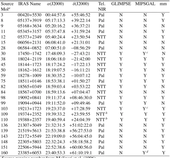
Table 1.1. List of Sources
Source IRAS Name α(J2000) δ(J2000) Tel. GLIMPSE MIPSGAL mm
Mola NIR 3 00420+5530 00:44:57.6 +55:46:52 Pal N N Y 8 05137+3919 05:17:13.3 +39:22:14 Pal N N Y 9 05168+3634 05:20:16.2 +36:37:21 Pal N N N 11 05345+3157 05:37:47.8 +31:59:24 Pal N N Y 12 05373+2349 05:40:24.4 +23:50:54 NTT N N Y 15 06056+2131 06:08:41.0 +21:31:01 Pal N N N 28 06584−0852 07:00:51.0 −08:56:29 Pal N N N 30 17450−1742 17:48:09.3 −27:43:21 NTT Y Yc N 38 18024−2119 18:06:18.0 −21:42:00 NTT Y Y Y 45 18144−1723 18:17:24.2 −17:22:13 NTT Y Y Y 50 18162−1612 18:19:07.5 −16:11:21 NTT Y Y N 59 18278−1009 18:30:35.2 −10:07:12 Pal Y Y Y 75 18511+0146 18:53:38.1 +01:50:27 Pal Y Y Y 82 18565+0349 18:59:03.4 +03:53:22 NTT Y Y N 84 18567+0700 18:59:13.6 +07:04:47 NTT N N N 98 19092+0841 19:11:37.4 +08:46:30.0 NTT Y Y Y 99 19094+0944 19:11:52.0 +09:49:46 Pal Y Y N 103 19213+1723 19:23:37.0 +17:28:59 NTT Y Yc Y 109 19374+2352 19:39:33.2 +23:59:55 NTTb Y Y Y 110 19388+2357 19:40:59.4 +24:04:39 NTTb Y Y Y 136 21307+5049 21:32:31.5 +51:02:22.0 Pal N N Y 139 21519+5613 21:53:38.8 +56:27:53.0 Pal N N Y 143 22172+5549 22:19:09.0 +56:04:45.0 Pal N N Y 148 22305+5803 22:32:24.3 +58:18:58.2 Pal N N Y 151 22506+5944 22:52:38.6 +60:00:56.0 Pal N N Y 160 23385+6053 23:40:53.3 +61:10:19.1 Pal N Yd Y
aSource running number from Molinari et al. (1996). bImaged only in K
s.
cImaged only in 24 µm.
I Part
Near InfraRed: low mass clusters
2.1 Observations and data analysis
Program fields are listed in Table 1.1 and were imaged in J, H, and Ksbands. A total of
15 fields were observed in three nights in November 1998 at the Palomar 60-inch telescope equipped with a 256×256 NICMOS-3 array of pixel scale 0.((62/pix and total FOV 2.(6×2.
(6. The remaining 11 fields were observed in 3 nights in August 2000 at the ESO-NTT
using the 1024×1024 SOFI camera with a pixel scale of 0.((29/pix and a total FOV of 4.
(9×4.(9. Standard dithering techniques were used to minimize the impact of bad pixels and
optimize flat-fielding, allowing us to achieve for each field a total of 5min integration time per band (in the central portion of the observed field) within an area of 3.(5×3.(5 of Palomar observations, and 20min (10min for the band Ks) at NTT of a total covered area of 6.(5×6. (5. Suitable calibration sources from the list of Hunt at al. (1988) were observed regularly
during the observations to track atmospheric variations for different airmasses. Standard stars and target fields were observed at airmasses no greater than 1.7 at NTT, and 1.3 at Palomar; we determined average zero-point magnitudes for each night and used them to calibrate our photometry. For each field, the images in the three bands were registered and astrometric solutions were determined using a few bright optically visible sources.
The Ks images for all observed fields, with superimposed submillimeter continuum
emission distribution when available (Molinari et al. 2008a) are available online1 2.1.1 Point source extraction and photometry
The extraction and photometry of point sources for all images were completed using the IRAF package. The r.m.s of the background signal and the FWHM of point sources were measured throughout the images to characterize the image noise and PSF properties; these parameters were fed to the DAOFIND task for source extraction, where a detection thresh-old of 3σ was used for all images. Sources with saturated pixels were excluded from the analysis; the linearity of the system response was checked a posteriori comparing, both for the Palomar and the NTT data, the magnitudes obtained to those from 2MASS using a few stars with magnitudes reaching up to the maximum values found in our photometry files; the relations between the 2MASS magnitudes and ours in the three bands were found to be linear over the entire magnitude range of the detected sources. There were clearly brighter
1at http://galatea.ifsi-roma.inaf.it/faustini/maps/
objects in the various fields, but their peaks were already flagged as saturated and excluded from the detection process.
The photometry of sources is difficult to determine in very dense stellar fields such as the inner Galactic plane, where all our target fields are located and the crowding is such that more than one source can enter either any plausible aperture chosen or any annulus used for background estimation. This problem is of course more extreme in the clustered environments close to detected sites of massive star formation (see Sect.2.2.1 below).
The first alternative approach that we tried to follow was PSF-fitting photometry that should be less affected by these problems. We chose a subsample of test fields with different levels of stellar crowding. In this procedure, an important aspect was the modeling of the PSF. To test this, we completed several trials selecting a variable number of point-like sources (from 3 to 30) of different brightness levels and different positions in the field. We found that the resulting PSF model was not particularly sensitive to the choice of numbers and/or brightnesses of the stars. However the results, were quite dependent on the mean stellar density of the field. The photometry was carried out using the ALLSTAR task, which was particularly suited to crowded fields. However, we also tested the other two tasks (PEAK and NSTAR) and obtained comparable results for most of the sources. We note, however, that in the most crowded areas in particular, the subtraction of the PSF-fitted sources from the image introduced two spurious effects: an unacceptably high level of residuals with brightness levels well above the detection threshold used and a significant number of negative holes, indicating that the PSF-fit included some background in the source flux estimation and therefore overestimated its value. Both effects are caused by both the limited accuracy of the PSF model that can be obtained for very crowded fields, where faint neighboring stars can enter the area where the PSF model is estimated, and the presence of a significant and variable background, which is quite common and expected for the Galactic plane. A similar conclusion was reached by Hillenbrand & Carpenter (2000) in their study of the inner Orion Nebula Cluster.
The second approach that we followed was standard aperture photometry. The choice of radii for both the aperture and the background annuli was of course extremely important. The optimum aperture should be neither too large to include nearby sources nor too small to truncate significantly the PSF and underestimate the flux significantly. We completed several attempts for one of the most crowded fields (Mol30, observed at NTT) with three different aperture radii equal to the PSF FWHM (typically 0.((7 at NTT and 1.((4 at Palomar in Ks), and twice and thrice this value. For each photometry run, we analyzed the source
flux distribution and, as expected, the median flux was found to increase with increasing aperture radius. Increasing the aperture from one to two PSF FWHMs increased the me-dian source flux by an amount compatible with the inclusion of the first ring of an Airy diffraction pattern. In contrast, when the aperture radius was increased to a factor of three higher than the PSF FWHM, the flux increase was far higher than could be attributed to the additional fraction of the Airy profile entering the aperture, and must therefore have been caused by the inclusion of nearby sources. We adopted an aperture radius equal to the PSF FWHM to minimize neighbor contamination, and then applied an aperture correction factor to the fraction of the PSF removed by the aperture; this was estimated by multi-aperture photometry (starting from a size of 1 FWHM) on relatively isolated stars in the target fields.
Given the crowding of our fields, a further effect to be corrected for is the possible contamination by the tails of the brightness profiles of neighbouring stars. To quantify this contamination, we created a grid of simulations with two symmetric Gaussians with a wide
variety of peak contrasts and different reciprocal distances. We computed the fraction of the Gaussian profile of the neighbouring source within the photometry aperture centered on the main source, and hence generated a matrix of photometry corrections for different source distances and peak contrasts. We then processed the magnitude file produced by the aperture photometry task and for each source we applied a magnitude correction depending on the presence, distance, and contrast ratios with respect to other neighbouring stars.
In spite of the various issues discussed above, the photometric data obtained with the two methods were in good agreement with each other, apart from at faint magnitudes. For these faint objects, we consistently found that the PSF photometry tends to produce brighter magnitudes (and hence stronger sources) than the aperture photometry; this effect can be easily understood from our finding (see above) that the subtraction of PSF-fitted sources always leaves negative holes in the residual image, and this effect is far more important for faint stars. We thus decided to adopt the magnitudes determined from aperture photometry.
For each target field, we estimated the limiting magnitude (LM) using artificial star ex-periments. The fields were populated using the IRAF task ADDSTAR with 400 fake stars with magnitudes distributed in bins of 0.25 mag between values of 15 and 21; the percent-age of recovered stars as a function of magnitude provides an estimate of the completeness level of our photometry. The star recovery percentage was not found to decrease monoton-ically with increasing magnitude because fake stars can also be placed very close to bright real stars and then go undetected by the finding algorithm. However, we find that the limit of 85-90% recovery fraction is reached on average at around J=18.7, H=17.7, and Ks=17.4
for NTT images, and J=18.0, H=17.3, and Ks=16.6 for Palomar images. We found that the
typical photometric uncertainty is below 0.1mag close to the limiting magnitude.
To verify the integrity of our photometry, we compared our magnitudes with those ex-tracted from 2MASS point source catalog for all the fields in our sample. Considering the differences in spatial resolutions between 2MASS and the telescopes used for our observa-tions, this comparison was limited to 2MASS point-like sources associated with a single source in the Palomar or NTT images. The median differences with respect to 2MASS for the various fields are of the order of−0.1, −0.2 and −0.3 mag for J, H, and Ksbands,
respectively. Within each field, the scatter around these median values is∼ 0.1 mag in all three bands, confirming the internal consistency of our photometry. Noticeable departures (∼0.5 mag) of the median difference with 2MASS from the above values are observed for the field of source Mol11 (Palomar), and for sources Mol103, Mol109 and Mol110 (NTT). However, the latter sources were observed on the same night, observations for which our log registered as not good due to sky variations that were not tracked by night-averaged zero points. We emphasize again, however, that these are systematic differences with respect to 2MASS in this limited number of cases; the r.m.s. scatter about these median differences are∼ 0.1 mag in all bands and this should provide confidence that the internal consistency of the photometry in each field is preserved. We then decided to rescale our photometry to the 2MASS photometric system to remove these systematic effects. The (J-H) and (H-K) color differences between 2MASS and our photometry are not correlated with the magni-tude, so that no magnitude-dependent color effect is introduced in this rescaling.
2.2 Results
2.2.1 Cluster Identification
The identification of a cluster results from the analysis of stellar density in the field. Since our target fields are sites of massive star formation associated with local peaks of dust column densities and hence of visual extinction, the Ksimages are clearly more suited for
this type of analysis.
Stellar density maps were compiled for each field by counting stars in a running boxcar of size equal to 20((. The box size was determined empirically to enhance the statistical significance of local stellar density peaks and to maximize the ability to detect the clusters. Larger boxes tend to smear the cluster into the background stellar density field decreasing the statistical significance of the peak, which may lead to non-detection of a clearly evident cluster, particularly in the rich inner Galaxy fields. Smaller boxes produce noisy density maps where the number of sources in each bin starts to be comparable to the fluctuations in the background density field caused either by intrinsic variations in the field star density or to variable extinction from diffuse foreground ISM in the Galactic Plane (where all of our sources are located). For most of our objects in the outer Galaxy, this analysis is used to locate the position of the peak stellar density, since the clusters are obvious already from visual inspection. For the remaining fields, the density maps are used to ascertain the presence of a cluster; toward the inner Galaxy in particular, the density maps tend to show more than one peak at comparable levels. It is important to remember, however, that this is a search for stellar clusters toward regions where indications of active star formation are already available, and this information can be used. In particular, the coincidence of these peaks with cold dust clumps traced by intense submillimeter and millimeter emission (Beltrán et al. 2006; Molinari et al. 2008a) is critical before we can consider the density peak to be a true feature associated with the star formation region. Casual association is excluded by the high number of positive associations (see Table2.1).
As further confirmation of the positive detection of a cluster we compiled radial stellar density profiles where stars were counted inside annuli of increasing internal radius and constant width and then divided by the area of the annuli (Testi et al. 1998); uncertainties were assigned assuming Poisson statistics for the number of stars in each annulus. We then assigned a positive cluster identification if the radial profile exhibited at least two annuli that had values above the background. To refine the location of the density peak, we repeated the radial density profile analysis starting from several locations within 10((of the peak derived from the density maps; the location that maximizes the overall statistical significance of the annuli was then assigned to the cluster center. Figure 2.1 shows the typical footprint of a cluster, where the stellar density is plotted as a function of distance r from the start location; the density has a maximum at r=0 and decreases until it reaches a constant value, which is the average background/foreground stellar density.
There were two exceptions in this analysis. The first was for source Mol160. The Ks
-band image shows clear stellar density enhancement in a semi-circular annulus surround-ing the northern side of the dense millimeter core, which appears devoid of stars. This stellar density enhancement is coincident with the emission patterns visible in the mid-IR (Molinari et al. 2008b), so is clearly a stellar population associated with the star-forming region. Since the millimeter peak is at the center of symmetry of the semi-circular stellar distribution, we consider this tobe the center of the cluster. This is only for completeness,
since we cannot say whether the low density of stars at the millimeter peak is an effect of extreme visual extinction or reflects an intrinsic paucity of NIR-visible forming stars, as the proposed extreme youth of the massive YSO accreting in its depth would seem to suggest (Molinari et al. 2008b).
The second exception was for source Mol8. The stellar density analysis shows two peaks that are coincident with two distinct dust cores; we therefore assumed the presence of two distinct clusters, rather than a subclustering feature within the same cluster. The radial density profile analysis could not be used here, so we fit elliptical Gaussians to the peaks in the density maps, allowing for an underlying constant level representing the back-ground stellar density. The resulting cluster richness was obtained by integrating the fitted Gaussian, and the cluster radius was taken to be equal to the fitted FWHM (the fitted Gaus-sians were nearly circular).
Figure 2.1. Stellar density (in stars/pc2), for Mol28, as a function of the radial distance (in parsecs)
from cluster center. Error-bars are computed as the Poissonian fluctuations of source counts in each bin.
Always following Testi et al. (1998), we determined the richness indicator of the clus-ter Icby integrating the background-subtracted density profile; the cluster radius was taken
to be the radial distance from the start location where the density profile reaches a con-stant value. This richness indicator is a very convenient figure to use when no detailed information is available for each single star in the region and the membership of the cluster cannot be established for each single star. These values are reported in Col. 3 of Table2.1 for all fields where a cluster has been clearly revealed. Column 1 gives the target name (cf. Table 1.1); its kinematic distance is listed in Col. 2. The parameter Nobs (Col. 4) is
the number of cluster members derived (see Sect. 2.3.1 below) from the integration of the background-subtracted Ks luminosity function (hereafter KLF, see Sect. 2.3.1). Also
re-ported in Col. 8 is the mass of the hosting molecular clump; this was derived from the cold dust emission as reported in Molinari et al. (2008a, 2000), integrated over the en-tire spatial extent of the cluster; conversion into masses was achieved based on the op-tically thin assumption and by assuming T=30 K, β = 1.5 (Molinari et al. 2008a), and a mass opacity κ230GHz = 0.005cm2g−1 which corresponds to a gas/dust weight ratio of
100 (Preibisch et al. 1993). The IRAS source bolometric luminosity, Col. 9, is taken from Molinari et al. (1996, 2000, 2002, 2008a); in Col. 10 we list the AV at the peak cluster
po-sition estimated from submm observations (Molinari et al. 2008a, 2000). In Cols. 11 and 12 the coordinates of the centers of the identified clusters are reported. Columns 6 and 7 contain parameters that are described later in the text (see Sect.2.2.2).
T able 2.1. Results for cluster detection Sou. d a Ic Nob s Rclu Pre-MS Mga s Lbol AV peak Cluster Center Mol kpc pc CC (%) CM (%) M! 10 3L ! mag α (J2000) δ(J2000) 3 2.17 78 78 1.7 34 99 910 12.4 18 00:44:57.4 + 55:47:20.0 8A 11.5 25 30 1.3 37 27 1650 57.0 18 05:17:13.8 + 39:22:29.7 8B 11.5 27 24 1.3 9 4 1780 5.5 8 05:17:12.0 + 39:21:51.8 9 6.2 7 7 0.6 16 − g − 24 − 05:20:16.9 + 36:37:22.0 11 2.1 51 48 0.5 12 41 360 4.6 35 05:37:47.7 + 31:59:24.0 12 1.6 12 13 0.3 0 30 72 1.6 46 05:40:24.4 + 23:51:54.8 15 1.5 64 61 0.3 34 − g − 5.8 − 06:08:41.0 + 21:31:00.0 28 4.5 75 75 1.0 58 95 220 9.1 4 07:00:51.5 − 08:56:18.2 30 0.3 200 e no cluster detected b -0.14 − − − 38 0.5 − 5 no cluster detected c -h 0.19 40 −− 45 4.3 28 27 0.5 68 19 1340 21.2 77 18:17:24.1 − 17:22:12.3 50 4.9 46 43 0.6 36 41 80 17.3 25 18:19:07.6 − 16:11:21.0 59 5.7 0 no cluster detected c -h 11 29 −− 75 3.9 8 7 0.7 37 24 1310 13.3 38 18:53:38.1 + 01:50:26.5 82 6.8 8 10 0.3 0 52 590 15.4 52 18:59:03.2 + 03:53:16.7 84 2.2 21 21 0.3 0 54 28 4.3 15 18:59:14.3 + 07:04:52.3 98 4.5 6 no cluster detected f -h 9.2 68 −− 99 6.1 45 38 0.9 49 − g − 37.3 − 19:11:51.4 + 09:49:35.4 103 4.1 105 107 0.7 46 87 510 28.2 42 19:23:36.2 + 17:28:58.1 109 4.3 19 17 0.5 dd 1030 26.7 90 19:39:33.0 + 24:00:21.3 110 4.3 23 20 0.5 dd 400 14.8 55 19:40:58.5 + 24:04:36.3 136 3.6 21 19 0.6 18 52 230 4 21 21:32:31.4 + 51:02:23.1 139 7.3 25 24 1.2 10 31 1870 1.35 20 21:53:39.2 + 56:27:50.7 143 5.0 25 22 0.8 10 76 630 7.8 26 22:19:09.0 + 56:04:58.7 148 5.1 43 41 0.9 43 64 22 7.8 13 22:32:23.4 + 58:19:01.3 151 5.4 15 14 0.9 12 30 2020 25 40 22:52:38.3 + 60:00:44.6 160 5.0 36 34 1.3 30 76 1830 16 32 23:40:53.1 + 61:10:21.0 aKinetic distance using the rotation curv e from Brand & Blitz (1993 ). bStellar density analysis inconclusi ve due to extreme cro wdedness of this fi eld. cStellar density re veales no peaks close to the IRAS position or the submm peak. dOnly observ ed in Ks . eDetection refused due to extreme fi eld comple xity (see te xt). fDetection refused because only 1 annulus in the radial density pro fi le is abo ve background (see te xt). gNo extinction estimate is av ailable due to lack of submm information to ev aluate de-reddening correction. hExtinction estimate is av ailable from single-pointing submillimeter data (Molinari et al. 2000 ) but not from maps, so that a reliable clump mass estimate is not possible.
Following the procedure described, a cluster was detected within 1(of the IRAS posi-tion for 22 out of the 26 observed fields (85% detecposi-tion rate). In two cases (Mol38 and Mol59), the stellar density map does not show a clear peak above the fluctuations of the field stellar density. For Mol 98, the radial density profile only shows one annulus above the background, and therefore fails the criterion that the stellar density enhancement should be resolved significantly above the background in two annuli. In one case (Mol30), several stellar density peaks were found in proximity to the IRAS source, but the lack of infor-mation about the submillimeter/millimeter continuum prevents us from drawing any firm conclusion.
Figure 2.2 shows Ic as a function of the peak AV and suggests that with higher dust
extinction, we may find it more difficult, or it becomes less likely, to detect a cluster at 2.2 µm.
Figure 2.2. Cluster richness indicator Icas a function of AVat the cluster center; for a few detected clusters, we do not have an estimate of AV).
Our detection rate is quite high and this implies that young stellar clusters in sites of intermediate and massive star formation are ubiquitous. While this was established for relatively old Pre-MS systems such as Herbig Ae/Be stars (Testi et al. 1999), we hereby verify that this is also true in much younger systems, where the most massive stars may even be in a pre-Hot Core stage (Molinari et al. 2008a).
Our detection rate is higher compared to other similar searches of stellar clusters toward high-mass YSOs. For example Kumar et al. (2006) used the 2MASS archive and reported a rate of 25% (rising to 60% when neglecting the inner Galaxy regions) toward a larger sample, which also includes the sources of this work; in particular, we detect all clusters
also detected by Kumar et al. and in addition we reveal clusters toward 13 objects for which Kumar et al. report no detection. The reason for this discrepancy may be because we obtained dedicated observations, while Kumar et al. used data from the 2MASS archive; the diffraction-limited spatial resolution of our data is between a factor of 4 and a factor of 10 better with respect to 2MASS, and this certainly facilitates cluster detection especially in particularly crowded areas such as the inner Galactic plane. To test this hypothesis, we degraded the NTT Ksimage of Mol103, also considered in Kumar et al., to the 2MASS
resolution; extraction and photometry were performed as outlined above but the search for a cluster based on the stellar radial density profiles revealed no cluster. The estimated number of members (corrected for the contribution of fore/background stars) for 7 out of the 10 clusters detected both by us and by Kumar et al. was at least a factor of two less in the latter study.
Kumar & Grave (2008) conducted a similar study on a large sample of high-mass YSOs, that included some of our sources, using data from the GLIMPSE survey (Benjamin et al. 2003). They detect no significant cluster around any targets in a sample of 509 objects. As the authors say in their paper, however, GLIMPSE data are sensitive to 2-4 M! pre-main sequence stars at the distance of 3 kpc. Based on color-magnitude analysis (see later below), our mass sensitivity is of the order of 1 M! at a distance of 3.6 kpc and ∼0.6 M!at a distance of 2.1 Kpc. Probing longer wavelengths, GLIMPSE is likely to be more sensitive to younger sources compared to the classical J, H, K range, which also samples relatively older pre-MS objects. The combination of sampling higher-mass (and hence rarer stars because of the shape of the IMF) and relatively younger stars (which, as indeed our analysis finds, may not be the majority in a young cluster) may plausibly be the reason for the negative cluster detection results of Kumar & Grave.
The distribution of the radii of the detected clusters indicated by a full line in Fig.2.3; the median value is 0.7 pc. The dashed histogram (which refers to the upper X-axis) shows the distribution of the cluster richness indicator Ic, with a median number of stars of 27.
We note that the value of Ic for many of our clusters is less than the limit of 35 suggested
by Lada & Lada (2003) to be a bona fide cluster. This definition stems from the argument that a less rich agglomerate may not survive the formation process as an entity. Our in-terest, however, is to investigate the spatial properties of the young stellar population in a star-forming region at the time of active formation, without worrying about its possible per-sistence as a cluster at the end of the formation phase. However, we prefer not to introduce a new term to identify the structures that we see and still use the term cluster, although in a milder way than Lada & Lada.
2.2.2 Properties of identified clusters
We first derive qualitative measurements related to the nature of the identified clusters using simple diagnostic tools such as color-color and color-magnitude diagrams. These diagrams have been drawn for all detected clusters and are available in electronic form; we illustrate here the particular case for Mol28.
Color-color analysis
Figure 2.4 shows the [J-H] versus [H-Ks] diagram for all sources detected within a
Figure 2.3. Distribution of the cluster radii in parsecs (full line) and the cluster richness indicator
Icin number of stars (dashed lines); the median values for the two distributions are 0.6 pc and 37 stars, respectively
detected in all three bands, the arrows representing sources with lower limits (to their mag-nitude) in the J band. The plot shows more stars than the Ic value reported in Table 2.1
because we also include the fore/background stars that cannot be individually distinguished from the true cluster members. A significant fraction of the sources have colors compatible with main-sequence stars that have a variable amount of extinction reddening (computed by adopting the Rieke & Lebofsky (1985) extinction curve), but many sources have colors that are typical of young pre-MS objects with an intrinsic IR excess produced by warm circumstellar dust distributed in disks (Lada & Adams 1992). The set of dotted curves rep-resents the locus of two-component black bodies with temperatures as indicated at the start and end of each dotted line; along each curve, the relative contribution of the the two black bodies is varied. These curves mimic the effect of a temperature stratification in the dusty circumstellar envelopes, and the presence of sources in the area covered by these curves is an indication of the presence of warm circumstellar dust.
A straightforward indication of the youth of the cluster may be provided by the fraction of sources that are not compatible with being reddened MS stars, i.e., those with IR excess. The number of stars with an IR excess is normalized to the total number of stars detected in the cluster area, corrected for the expected number of fore/background stars estimated from the areas surrounding the cluster (but still in the same imaged field). To be conservative we extend the region of the MS by 0.2 magnitudes to the right corresponding to about a 2σ uncertainty in measured magnitudes. This ratio is reported as a percentage value in Col. 6
Figure 2.4. [J-H] vs [H-Ks] diagram for Mol28. Upward pointing arrows are the sources not
detected in J. The continuous curve at the bottom-left represents the main sequence, while the dashed grey lines represent the effect of reddening ( Rieke & Lebofsky 1985) for variable amounts of extinction as indicated along the lines. The dashed-dotted black line is the black-body curve, and the dotted curves are two-component black-body curves with varying relative contribution (respectively, from the inner to the outer curve, 3000-1500K, 3000-1000K, 3000-900K and 3000-500K).
of Table 2.1.
Color-magnitude analysis
Additional evolutionary indications of the detected clusters may be derived from the Ks
-[H-Ks] diagram, reported for Mol28 in Fig. 2.5. Compared to the main sequence (the leftmost
almost vertical curve in the figure) a significant fraction of the sources are on its right, where the evolutionary tracks for Pre-MS sources (Palla & Stahler 1999) can also be found, and could therefore be interpreted as very young pre-MS objects. The distribution of sources in the diagram spans a much larger region than that covered by the Pre-MS isochrones, because of the combined effect of extinction reddening and IR excess. The extinction effects can be seen from the dotted lines originating in the main sequence and extending toward the bottom-right for increasing values of AV. On the other hand, the presence of
a warm dusty circumstellar envelope implies an increase in both absolute emission and SED steepness, which would shift a pure photosphere toward the top-right of the diagram (as shown by the arrow labeled ’IREX’ in Fig. 2.5). In a similar way to the color-color analysis, it is impossible to estimate the age of individual stellar sources based on their location on the pre-MS isochrones, because we do not know the amount of AV by which
we should de redden each object. We follow a conservative approach by dereddening each object using half of the exctinction estimated for each location from millimeter maps; this corresponds to placing each object midway through the clump.
Figure 2.5. Ks vs [H-Ks] diagram for Mol28. The leftmost curve represents the main
se-quence, while the dashed lines represent the effect of reddening for variable amounts of extinction. Isochrones from Palla & Stahler (1999) are also indicated with full lines for different Pre-MS ages. The arrow labeled IREX indicates the direction of change due to IR-excess (see Sect. 2.3.2). Right-ward pointing arrows represent those sources not detected in H. Symbols in grey color indicate sources with IR excess as determined from the color-color diagrams (see Fig. 2.4).
A further correction is to remove the IR excess for those sources, which is apparent in the color-color diagram (of fig. 2.4), estimated using the formulation suggested by Hillenbrand & Carpenter (2000), and used later in this work (see Sect. 2.3.2). The ratio of pre-MS stars to the total in each cluster area will remain contaminated by fore/background stars; to estimate this contamination, we choose an off-cluster area in the same imaged field and simply compute the ratio of sources with pre-MS colors to the total (in these off-cluster regions in which there is no significant reddening to correct for). for each cluster, Col. 7 of Table 2.1 reports the fraction of stars (detected in the cluster area in all three bands) situated more than 0.2 mag to the right of the MS after the various corrections have been applied.
2.3 Initial mass functions and star formation histories
As is apparent from the qualitative analysis presented in the previous paragraphs, the diag-nostic power of our observations is limited because we do not know which objects in the
cluster area are true cluster members nor the precise amount of dust extinction (originating within the hosting clump) and IR excess (originating in the immediate circumstellar envi-ronment) pertaining to each source. Without this detailed knowledge of individual stars in the clusters, fundamental quantities such as the initial mass function (IMF) and the star formation history (SFH) cannot be derived directly from, e.g., the Ksluminosity function
(KLF). We are compelled to obtain these using statistical simulations of clusters based on different input parameters and performing a statistical comparison between synthetic and observed KLFs and HKCFs.
We first derive the observed KLFs from the observations. We then illustrate in detail the model used for the cluster simulations, exploring the sensitivity of the results to a wide range of input parameters finally, modeled and observed KLFs are compared to infer statis-tically the IMF and SFH for our clusters.
2.3.1 Observed Ksluminosity functions
The KLF of each cluster is obtained by simply counting all detected sources within the cluster area as identified from the cluster density profile (see Sect.2.2.1). In a similar way to the other diagnistic tools (Sects.2.2.2 and 2.2.2), the KLF is contaminated by field stars that cannot be individually identified. To account for the field star contamination in a statistical way we subtract from the KLF that was compiled for the cluster area, the KLF for a region outside the cluster area but still in the same imaged field, after normalising the different areas. The regions in which the field star KLF is compiled have a lower extinction with respect to the cluster KLF, so the background contribution to the cluster KLF is likely to be overestimated. Field-subtracted KLFs for all clusters are available online2.
The integral of the KLF provides an independent estimate of the number of cluster members, and these values are reported as Nobs in Table 2.1. Their agreement with the
richness indicator Ic confirms the consistency of our analysis. All KLFs show a dominant
peak that is always close to the completeness limit, showing that our observations are in-sufficiently sensitive to the low-mass stellar component of our clusters. Many of the KLFs present a separate small peak at low magnitudes (one or two sources at most, on average). Could this be caused by confusion because of source crowding and insufficient spatial res-olution ? For each cluster, we studied the distribution of distances of each star from its nearest neighbour and found that there are two types of distributions, reported in Fig.2.6. In the first type (full line in figure), the distribution has a peak corresponding to an inter-star distance significantly higher than the value corresponding to half the PSF FWHM (the full vertical line); in this case, the suggestion is that all cluster members have been resolved from their neighbour. In the second type (dashed line in the figure), the distribution has its peak very close to half the PSF’s FWHM (the dashed vertical line), indicating that source blending should certainly be considered possible. We verified that all clusters with a dis-tance distribution of the second type do exhibit a second faint peak at high brightness in their KLFs, therefore confirming that this feature is an artifact of the relatively low spatial resolution, which in some cases is insufficient to resolve all cluster members.
Figure 2.6. Distribution of identified sources as a function of nearest-neighbor distance (D) for two
of our examined fields (Mol28 dashed line and Mol103 full line).
2.3.2 Synthetic KLF. Synthetic cluster generator: a near-IR cluster simula-tor
As already mentioned, we cannot derive masses and ages from our data alone. We thus de-veloped a model to create statistically significant cluster simulations obtained for different assumptions of IMF and SFH (source ages and their distribution), and compare the syn-thetic KLFs with the observed field-subtracted KLFs. This model we called the synsyn-thetic cluster generator (SCG).
SCG: model description
A cluster is created by adding stars whose masses and ages are assigned via a Monte-Carlo extraction according to the chosen IMF and SFH; the pre-MS evolutionary tracks of Palla & Stahler (1999) are then used to convert them into J, H, and Ksmagnitudes. The 3D
distribution of stars is obtained by randomly choosing for each star a set of x,y,z coordinates using the observed stellar density profile (see Sect. 2.2.1), approximated to be a radially symmetric Gaussian, as weight-function; using submm continuum images, this is needed to assign the proper column of cold dust "required" to extinguish the near-IR radiation. Other analytical functions could have been used, e.g., a King profile, but the statistics of our clusters are insufficiently high to explore the effect of different radial profile assumptions.
To convert the submm flux into dust column density, we used the dust temperature and emissivity exponent β determined in Molinari et al. (2000); mean values from the latter
work were adopted for those fields not covered by our work.
To properly simulate the pre-MS stars, we also need to include the effect of an IR excess caused by warm dust in the circumstellar envelopes and disks. We used the distri-bution (modeled as a Gaussian) of [H-Ks]ex color excesses as measured for a sample of
Pre-MS stars in Taurus, as used by Hillenbrand & Carpenter (2000), as a weight-function to randomly assign a [H-Ks]ex to each simulated star in our model; the Ks vs [H-Ks]ex
relationship adopted in the above mentioned work was then used to derive the H and Ks
excess-corrected magnitudes. The Ks magnitude of the synthetic star was then compared
with the limiting magnitude typical of the cluster being simulated to determine whether the star could have been detected in our observations. This procedure is repeated until the number of synthetic detectable stars equals the value of Icdetermined for our observations;
at this point, the cluster generation process is complete.
Since the simulation is based on Monte Carlo extraction of stellar mass, age, and posi-tion in the cluster, each independent run for a fixed set of input parameters can in principle result in very different outputs in terms of cluster luminosity, total stellar mass, maximum stellar mass, and synthetic KLF. To determine the statistical significance, the model is run 200 times for any given set of input parameters, and the median KLF is later adopted for comparison with the observed one. Clearly, the predictive power of this simulation model resides in its capability to characterize the cluster properties of any given parameter set. In other words, the distribution of the resulting quantities should not be uniform but peaked around characteristic values. We return to this point in Sect.2.3.2
SCG: input assumptions
We tested three different assumptions about the star formation histories in our cluster simulations. The first was to assume that stars in the cluster formed in a single burst-like event (hereafter SB) some t1 years ago. The explored range in the simulations is
103 ≤ t1 ≤ 108 yrs. The second was that the formation of stars proceeds at a constant
rate (hereafter CR) from a time t1 years ago to a time t2 years ago. The ranges explored
in the simulations are 104 ≤ t
1 ≤ 108 yrs and 103 ≤ t2 ≤ 107 yrs, where we always
as-sume that t1 > t2. The third possibility that we explored was a variation in the previous
assumption, where the star formation rate is not constant but varies with time as a Gaussian function (hereafter GR). Within the boundaries of the start and end of the star formation process, t1and t2that were varied as above, we also varied both the time tcof the Gaussian
peak in the range 103.7 ≤ tc ≤ 107.7 and Log10(σ) of the Gaussian-like SFH, which was
allowed to have one of two values 0.1 and 0.5.
We allowed three different choices of IMFs, i.e., Kroupa (1993); Scalo (1998); Salpeter (1955), with the latter modified by introducing a different slope for M<1 M!coinciding with that of the Scalo (1998) IMF; the three IMFs were labeled IMF1, IMF2, and IMF3, respectively. The IMF from Kroupa et al. provides a more accurate description of the low-mass end of the distribution, while the classical Salpeter IMF is flatter at low mass but heavier at intermediate and high masses (above 1 M!). The properties of the Scalo IMF is in-between the other two, resembling Salpeter’s one below 1 M!and above 10 M!, and Kroupa’s for 1 M!<M<10 M!.
SCG: predictive power
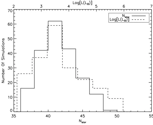
To verify our model’s predictive power, we completed 200 simulations for a cluster with a Salpeter IMF and a constant star formation rate with t1=106yrs and t2=104yrs. Figure 2.7
shows the distribution of the predicted number of stars and the total luminosity for the 200 simulations. The number of cluster members shows very little variation, as expected since the number of detectable stars is the parameter that we use to stop the simulation; on the other hand, the distribution of the total luminosity is not particularly peaked, as the central 3 bins containing about 60% of the simulations span almost two decades in luminosity.
Figure 2.7. Distribution of the predicted number of cluster members (full line) and total luminosity
(dashed line) for 200 SCG runs for Mol160 with a Salpeter IMF and a constant star formation rate with t1=106yrs and t2=104yrs.
On the other hand, the distributions for the total cluster stellar mass, and for the mass of the most massive member (see Fig. 2.8) are rather peaked and highlight a relatively higher predictive power of the model for these two quantities. It is to be noted that the distributions are rather skewed, suggesting that neither the mean nor the median are particularly suited to characterize the peak of the distribution. We indeed found that these quantities assume at their distributions peak a more representative value of mass and use them in the following discussion.
Concerning the reproducibility of the KLF, for each of the 200 runs the resulting KLF was fitted with a Gaussian function and the center, peak and σ were determined. Figure2.9 reports the distribution of these three parameters for the 200 runs and shows that all of them are remarkably peaked and symmetric. The formal r.m.s. spread for the three quantities, estimated via a Gaussian fit to the distributions in the figure, is ≈ 0.3 mag for the KLF
Figure 2.8. Distribution of the predicted total stellar mass (full line) and mass for the most massive
star (dashed line) in a cluster for 200 SCG runs for Mol160 (same inputs as in Fig. 2.7).
center, ≈ 12% for the KLF peak (about 1.2 sources out of a mean KLF peak of 10), and ≈ 0.25 mag for the KLF FWHM.
We completed a similar analysis for HKCF (H-Kscolor function; see Sect. 2.2.2).
Fig-ure 2.10 shows the distribution of Gaussian function centers, peaks and σ’s for HKCFs obtained for the same 200 runs used previously for the KLFs. Gaussian fits to the three distributions in the figure infer an r.m.s. that is ≈ 0.15 mag for the HKCF center and ≈ 0.14 mag for the HKCF FWHM, while the "peak" distribution is flatter and has an r.m.s. value of≈ 21% for the HKCF peak (about 3.2 sources out of a mean HKCF peak of 15). It is worthwhile to stress that since the position that is assigned to each simulated star in the cluster is different in each of the 200 runs of the model (for any given set of input parame-ters), the scatter in the properties of the synthetic KLFs and HKCFs also statistically tends to account for the effects of extinction variations in the cluster’s hosting clump, which may in principle be relevant in such heavily embedded systems (see Table2.1).
For a given set of input parameters, we conclude that the model results, have a good reproducibility, except concerning the total luminosity. The model therefore has a strong predictive power concerning the median properties of a synthetic cluster. The spread in KLF center magnitudes is indeed, less than the bin amplitude used in compiling the KLFs for the simulations (and is used in the remainder of the work); the median synthetic KLF therefore provides a good representation of the cluster luminosity distribution.
In conclusion, 200 simulation runs for each combination of input parameters (IMF and SFH) can provide a robust assessment of the statistical significance of the synthetic
observ-Figure 2.9. Distribution of the predicted center magnitude (full line - bottom X-axis scale), width
(dotted line - bottom X-axis scale) and peak value (dashed line - top X-axis scale) of the predicted Gaussian-fitted KLFs for 200 SCG runs for Mol160 (same inputs as in Fig. 2.7).
able properties (KLFs and HKCFs). Although the distributions for the KLFs’ (HKCFs’) parameters seem rather symmetrical, we adopt the median KLF (HKCF) of the 200 runs as a more reliable characterization for that particular parameters’ set. The use of the mean KLF (HKCF) for the comparison does not significantly alter the results.
Exploring the SCG parameter space: cluster parameters
After verifying the robustness of model results in independent runs for the same input parameters, we now measure the sensitivity of the model results to changes in these pa-rameters. We first concentrate on simulated cluster physical parameters (number of cluster members, total luminosity, stellar mass distribution), and in the next paragraph we examine how the KLFs and the appearance of the color-magnitude diagrams, which are the main observables used in our analysis, behave in this respect.
Number of stars Nstars- As a general rule, the older the cluster is allowed to be,
irrespec-tive of the detailed SFH adopted, the higher is the number of produced stars. This is easily understood since the SCG cluster formation is stops when the number of the Ks-detectable
stars equals the number of observed objects; if a cluster is old, the stars will be intrinsically fainter due to the shape of Pre-MS tracks and statistically less likely to extract stars bright enough to be detectable. As long as t1 ≤ 106 yrs, Nstars does not depend significantly on