CHAPTER 4 68

4. DATA ANALYSIS FOR FUSION CROSS-SECTION EXTRACTION

In this chapter the analysis of the experimental data collected by the procedures described in chapter 3 will be discussed. These data are of two kinds: the energy spectra measured by monitor detectors during the activation step; the X-ray spectra recorded after the end of the activation step that have been collected off-line several times, during a period of some months. In the following paragraphs will be described the procedures used for the ER production cross-sections extraction (at a given energy corresponding to a precise stack). The first step of this procedure is the reconstruction of the activity curve for a given ER charge Z. Next, this activity curve has been fitted in order to unfold the contribution of different isotopes (having different half-lives) and to find the activity A0 for each ER at the end of the activation step (which is linked to the number of produced ERs). Finally, the activity at the end of the activation step has been used to extract the production cross-section for each considered ER taking into account several parameters such as: the beam current profile as a function of activation time; the X-ray detection efficiency; the Kα fluorescence probability etc.

4.1 X-ray spectra

The collected data are stored in runs with durations from 15’ to 12h. Since in the first runs, immediately after the activation, the spectrum is dominated by ERs with short half-lives the data run must be divided into parts corresponding to short elapsed times. Indeed, in order to extract the activity as the ratio between the peak area and the duration of the run part, it is necessary that the activity can be considered constant in the time interval corresponding to the run part. For each acquired event the local time has been also recorded on disk allowing to determinate with a good precision the time coordinate of the run part with respect to the end of the activation. In the assumption of a constant activity during the entire run part, the time coordinate is the mean value between the start tstart and the stop tstop of the run part:



t  tstart tstop

2 (4.1)

After a reasonable time from the end of the activation step the run duration is shorter than the dominant ERs half-lives hence the run division is not necessary any more. When the

ERs half-lives in the stack are very long two or more consecutive runs can be merged in order to obtain a sufficient statistics.

As shown in figure 4.1 the measured spectrum for a generic stack shows a background that has been removed by fitting it in the spectrum regions without peaks. For the background fit an exponential function has been used:



y  Ce

where C and k are fitting parameters. Fitting the background with different functions it has been found that the exponential is the best background approximation that preserves the known ratio between the Kα and the Kβ intensities shown in table 3.4.

Called with



x the mean position of a peak and with L the width of the peak (about 4σ), the

background area below the peak B is



B 





C

k

e

_e

 e





The background removal adds an indetermination to the peak area equal to the error done in the determination of the background area below each peak. This error is calculated applying the error propagation to the equation (4.3)

 B2 B2  C2 C2  k2 k2  x 2_{ k}2 _(4.4)

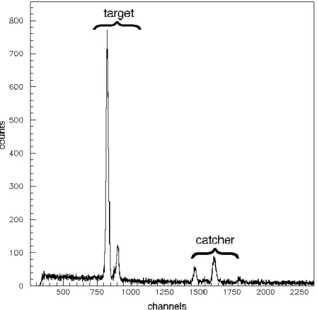
In figure 4.1 are shown energy peaks from the ERs produced by the reaction of 6Li with 64_{Zn (in particular the dominant gallium Kα and Kβ lines) and the peaks due to other ERs} produced in the reaction of the same beam with other elements in the stack. In the specific case of the niobium catcher and the bismuth layer the characteristic X-ray energies of these other peaks are high enough to be separated from the peaks of interest. When the catcher material in the stack is the holmium some X-rays corresponding to the Ho L-lines are in the same energy range of the electron capture X-rays emitted by the ERs. The more intense holmium peak has a mean energy low enough to be fitted separately (6.7 KeV). Consequently the contribution of the other two lines (at 7.5 and 7.9 KeV), which are

respectively the 64% and the 20% of the fitted peak, can be subtracted from the peaks of interest. This subtracted contribution is typically about the 4% of the lines of interest intensity. In table 4.1 are listed the isotopes of interest.

Fig. 4.1: The X-ray spectrum as it appears before the analysis. It can

be seen the background, the peaks produced in reactions with the target (the dominant gallium Kα and Kβ) and the peaks due to reactions with the other elements in the stack.

The peak integration has been done fitting the spectrum as the sum of several overlapped Gaussian functions. In order to reduce the number of free parameters, the ratio Kα/Kβ shown in table 3.4 has been imposed as ratio between the areas of the two corresponding Gaussian functions. In addition, supposing that the peak width is mostly correlated to the detector energy resolution, the σ parameter has been imposed the same for all the peaks. Since the energy calibration is known, the position of the peaks in the spectrum fit has been fixed. The only free parameters in the fit are the heights of all Kα peaks and their width that is the same for all peaks. In figure 4.2 is shown the result of the fit procedure on a spectrum from the 6Li@17.5 MeV activated stack measured about 10 days after the end of activation step.

This fitting procedure takes into account the partial superimposition of the Kα and Kβ peaks of ER having charge Z and Z+1.

Fig. 4.2: A sample fit of an X-ray spectrum. This spectrum has been

measured about 10 days after the activation of the 17.5 MeV stack with the 6_{Li beam. The Ka peaks of zinc,} gallium and germanium can be seen. The Kb peaks of zinc and gallium are covered by other peaks. On the other hand the germanium Kb peak can be seen on the right.

The fitting function for each peak is:



y  K  e

x is the fixed mean energy of the peak whereas σ and K are free parameters. The

relation between K, σ and the peak area AG is:



AG K  2 (4.6)

Hence it is possible to measure the number of detected Kα X-rays for each element all the run duration long. The indetermination ΔAG on this area is given by:

 AG AG       2 K2 K2  2 2 (4.7)

so the overall indetermination on the number of counts N = AG, considering the background removal error ΔB, the Gaussian fit error ΔAG and the statistical error, is:

 N N  B2 B2  A_G2 A_G2  1 N (4.8) 4.2 Activity

The electron capture decay follows the scheme:

 AZF  e _ A Z 1_{D } e (4.9)

where F is the father nucleus and D is the daughter nucleus. The activity curve is the variation of the measured activity with the time and follows the exponentially decrease of the decay law:



A  A₀et _(4.10)

where A is the contribution of the single isotope to the overall activity, A0 is the isotope activity at the end of the activation and λ is the isotope decay constant that is linked to the isotope half-life T½ by the relation:



ln 2

 

T₁ 2

(4.11)

The measured number of X-rays for each peak, N, is the result of the decay of different isotopes of the same element. Each isotope of the same element contributes to the overall activity of the element with its exponential curve and its decay constant, hence the overall

activity as a function of time is the sum of several exponential contributions. Plotting the activity curve in a logarithmic scale each isotopic contribution is a slope:



ln A

 

 

The overall activity measured for a specific element hence is the sum of as many slopes as the number of isotopes of that element are implanted in the stack. In order to determine the production cross-section for each isotope in the stack it is necessary to know the A0 activity at the end of the activation step for each of them. The A0 activities at the end of the activation step can be found by fitting the overall activity curve as the sum of its exponential contributions.

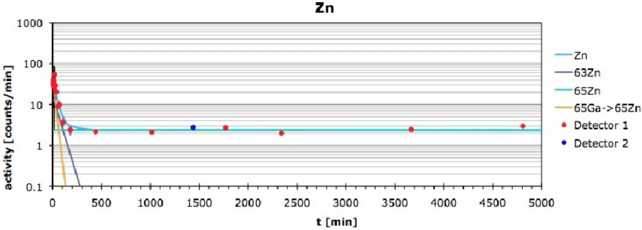
Fig 4.3: Overall activity curve as a function of the elapsed time from the end of the

activation for the Zn Kα peak, corresponding to the daughter nucleus Kα peak energy (Cu). See the text for details.

Fig 4.4: Overall activity curve as a function of the elapsed time from the end of the

activation for the gallium Kα peak, corresponding to the daughter nucleus Kα peak energy (Zn). See the text for details.

Fig 4.5: Overall activity curve as a function of the elapsed time from the end of the

activation for the germanium peak, corresponding to the daughter nucleus Kα peak energy (Ga). See the text for details.

As seen in paragraph 3.2 the overall activity A for each element is given by the equation (3.3) and it is not depending on the acquisition dead time. The pulser integration, needed for the activity, has been done by integration. Since two different detectors have been used the activities measured using detector 1 have been rescaled using the relative efficiency between the detectors.

The time position t of each measured activity is given by equation (4.1) and its indetermination is Δt = 2s since the indetermination on tstart and tstop is 1 second. As examples, in figures 4.3-4.5 the activity curves for each element measured in the 6_{Li@24MeV activated stack are shown.}

4.3 Feeding and activity fit

In some cases the daughter nucleus is in turn the father nucleus for a further electron capture decay. In this case, if λF is the decay constant of the father nucleus and λD the daughter one, the daughter activity AD follows the general law:



A

_{ A}









e

 e





 A

_e

A₀D _{are respectively the activities of the father nucleus and the daughter}

constant of the father nucleus is much smaller than the daughter nucleus one. In this case the formula (4.13) can be simplified as the sum of an exponential contribution with the father nucleus slope and the exponential contribution of the daughter nucleus. Hence the sequential decay between the isotopes of interest can be taken into account by fitting also the exponential contribution of the father nucleus in the activity curve. As an example, in the Zn activity curve is also fitted the 65Ga (15.2 minutes) exponential contribution because the 65Ga isotope decays into 65Zn (243 days). In order to determine the activity A0 at the end of the activation step it is necessary to fit the overall activity curve as the sum of its components eventually including the ones due to sequential decays.

In order to correctly fit the activity curve, first of all, the points corresponding to longest times elapsed from the activation has been fitted by the smaller slope (longer half-life). Then the points, which correspond to the sum of the activities of the two slowest elements, have been fitted by the sum of the previous slope and the one of the successive element. This procedure has been repeated for each slope from the longest half-life to the shortest one. In figures 4.6-4.8 are shown the fits and the different slopes contributions for the activity curves already shown in figures 4.3-4.5 respectively.

Observing table 3.1 there are some nuclei (67As, 65Ge, 63Ga, 61Zn), marked in red, with half-life smaller than the time needed to open the activation chamber and put the stack in front of the Si-Li drifted detector (~7’). During these operations the activity for the fastest nuclei is lost but their contribute to the fusion cross-section can be measured as an additional presence in their respective daughter nuclei, which have half-lives from 18’ to 3h.

Fig 4.6: Best fit of the overall activity curve as a function of the elapsed time from

the end of the activation for the zinc peak, corresponding to the daughter nucleus Kα peak energy (Cu). For each Zn isotope is shown the respective slope. See the text for details.

Fig 4.7: Best fit of the overall activity curve as a function of the elapsed time from

the end of the activation for the gallium peak, corresponding to the daughter nucleus Kα peak energy (Zn). For each Ga isotope is shown the respective slope. See the text for details.

Fig 4.8: Best fit of the overall activity curve as a function of the elapsed time from

the end of the activation for the germanium peak, corresponding to the daughter nucleus Kα peak energy (Ga). For each Ge isotope is shown the respective slope. See the text for details.

As result of the fit procedure one obtains the activity A0 exactly at the end of the activation step for each of the isotopes in the stack. In order to convert this information into a cross-section it is necessary to use the beam current profile extracted during the activation step.

4.4 Beam current profile

As seen in the previous chapter, the beam current profile during the activation step has been measured detecting the scattered particles from a thin gold foil placed before the stack. The spectra of the two monitor detectors have been divided into sub-spectra corresponding to the events collected every 10 seconds. Integrating the Rutherford peak on each sub-spectrum one can obtain the number of detected particles as a function of time. Taking into account the solid angle and the target thickness as described in paragraph 3.2, the current I is linked to the scattered particles by the relation:

 I  dt  M  d d       Ruth   (4.14)

where M is the integration of the Rutherford peak in the sub-spectra, ξ is the gold foil thickness,  d d       Ruth

is the Rutherford cross-section in the laboratory system and ΔΩ is the solid angle covered by the monitor detector

     2       2 d2 (4.15)

where ϕ is the monitor collimator diameter and d its distance from the gold foil.

In order to take into account the acquisition dead time the beam current value IM has been multiplied by the expected pulser, that is the product of the pulser frequency for the run duration ΔT (in minutes), and it has been divided by the integration P of the acquired pulser:



I  I_M 50  60  T

P (4.16)

In figure 4.9 it is shown a sample beam current profile from the 6Li @ 20 MeV run superimposing the two profiles extracted from the first (left) and the second (right) monitor. The average current profile information has been stored in an array of values each of them corresponding to a time bin of 10 seconds.

78

Fig. 4.9: The current profile extracted from the monitor detectors for the

6_{Li @ 20 MeV run. The current has been measured performing a Rutherford} scattering on a thin gold foil and detecting the scattered particles on two monitor detectors symmetrically placed with respect to the beam line. The left monitor and the right one are of different colors.

4.5 Production cross-section

The total fusion cross-section is the sum of the ER production ones that have been extracted using both the current profile and the activity value at the end of the activation step for each ER. The activity at the end of the activation A0 is linked to the number of father ER nuclei NX by the relation:



N_X  A0

 (4.17)

where λ is the decay constant of the specific ER, listed in table 4.1.

Since the electron capture decay is in competition with other decay modes and the ERs atoms does not de-excite only by the Kα lines emission but also emitting Auger electrons, the detected ERs are only a part of the total in the stack. To take into account this fact has been used the known absolute probability of a Kα X-ray emission per electron capture decay that is given by the fluorescence probability K, listed in table 4.1 for each isotope. As shown in the paragraph 3.3 the number of detected X-rays is less than the effective number of emitted X-rays and the ratio between these two quantities is the overall detection efficiency ε, which is the product of the geometric efficiency for the intrinsic efficiency. The ERs number for a given isotope at the end of the activation step hence results  N  A0  100 K_ 1  (4.18)

where ε = 0.083.

By the definition of cross-section σ:



N  IT (4.19)

where IT is the total number of incident particles and η is the target thickness in number of atoms for cm2 that is



 NA

A

1

1000 (4.20)

where NA is the Avogadro’s number, A the mass of the target element (64) and ξ the target thickness in g/cm2. Substituting the (4.20) and the (4.18) in the (4.19) (and considering that one barn is 10-24 cm2)



[mb]  A0A 1027

 K_ N_A I_T (4.21)

TABLE 4.1

Decay constant λ and fluorescence probability K for the detected Kα lines Isotope λ [min-1] K(Kα) [%] 62 Zn 0.0012476 37.60 63_{Zn 0.0180179 2.51} 65_{Zn 0.0000020 34.20} 65_{Ga 0.0456018 19.30} 66_{Ga 0.0012173 16.93} 67_{Ga 0.0001476 50.00} 68_{Ga 0.0102370 4.06} 66_{Ge 0.0051117 43.80} 67_{Ge 0.0366745 2.68} 68_{Ge 0.0000018 38.80} 69_{Ge 0.0002958 30.50}

The activation step duration is longer than the half-life of the more short-lived ERs produced in the reaction hence, during the activation step, a certain number of ERs decay

of the activation is the result of the competition between the production by reactions and the simultaneous decay of the produced ERs. In order to take in account this effect the equation (4.21) must be modified considering the production and the decay of the ERs during activation run steps of Δt = 10s. Each step of the calculation takes into account the number of produced ERs in the previous step. The total production cross-section is, in this case, proportional to the ratio between the measured activity A0 and the activity built considering the beam current profile AI

  A0 A_I  1027  K_ (4.22) where  A_I  A_i i





where ΔI(ti) is the value stored in a 10 seconds bin by the current profile analysis described in paragraph 4.4 and ΔAi the built activity at the i-th step.

The equation (4.22), with the step-by-step calculation in (4.24), allows extracting the production cross-section of each isotope detected in the stack. In figure 4.10 and 4.11 are shown the relative production cross-sections for the 6Li+64Zn and the 7Li+64Zn collisions respectively.

4.6 Statistical model calculations 4.6.1 Statistical model

As seen in chapter 1, in a fusion reaction the CN formation is followed by particle and photon emission leading to different ERs. The statistical model describes the CN de-excitation evolution in order to calculate the produced ERs distribution.

The fundamental condition needed by this model is the assumption that all the system degrees of freedom are statistically equilibrated before the decay. This condition is verified only if the CN survives for a time interval sufficient to make equiprobable all the quantum levels that the CN may occupy. All the possible decay channels become, in this way, equally probable. The process is determined by the conservation of the angular momentum, the parity and the father-daughter system energy. Moreover the process is determined by the transmission coefficients TL and by the level densities of both the father nucleus and the daughter one. Knowing these latter quantities it is possible to calculate the emission rates for the x particle with energy Ex.



R

dE







E

,J

,





h





E

,J

,





T

_E

 

dE





where E2, J2 and π2 are respectively the energy, the spin and the parity of the daughter nucleus and E1, J1 and π1 are referring to the father nucleus. ρ1 and ρ2 are the state densities of the father and the daughter nuclei, Lis the total angular momentum of the exit channel, Sx is the spin of the x particle and S  J₂ S_x is the total spin of the exit channel. The TL transmission coefficients can be calculated using the optical model.

The photon emission rate is



R

dE







E

,J

,





h





E

,J

,





E



hc















3

dE

Where Eγ=E2-E1 is the photon energy and σabs is the dipolar photon absorption cross-section. This cross-section can be characterized by one or two lorentzian functions depending on the cases.

The level density can be obtained in several ways. The simpler is the one at constant temperature





e

EEo T

where T is the nuclear temperature associated to the excitation energy that is used at low excitation energies. In other cases are added some corrections due to the shell and pairing effects, which are estimated by empirical fits for each nucleus. At high excitation energies the Fermi gas model is used:







E,J,







2J 1

12 U  T





a

h

2I













e

where I is the nucleus moment of inertia and



U  E   h

2_{J J 1}





2I  aT

2_{ T (4.29)}

where Δ is the pairing energy and T the nuclear temperature associated to the excitation energy E.

The computational statistical model simulations can be realized by a multi step gridded or a multi step Monte Carlo. In the former case, the E*/J plane is divided into cells for each father nuclei and it is possible to calculate the respective decay mode for each of these cells into a cell of the daughter nucleus E*/J plane. This step is repeated until the father nucleus has no longer the excitation energy or the angular momentum required to decay. In the Monte Carlo method the whole decay process for the CN is reproduced event by event. The formation probability for a CN in a state E*/J and the choice of the decay mode has been calculated following the formalism in (4.26) and (4.28). Even for this method the step is repeated several times. Differently from the grid method, the Monte Carlo method makes it possible to analyze the correlation among different quantities and allows calculating the energy spectrum and the ER angular distribution.

4.6.2 Comparison of data with statistical model code results

Since the two used projectiles 6Li and 7Li have low α separation energies (Sα[6Li]=1.48 MeV Sα[7Li]=2.54 MeV) it is expected that a non negligible fraction of the measured total fusion cross-section is due to ICF as already observed for similar systems as in the 6,7Li+59Co systems [12]. Some information about the ICF contribution to total

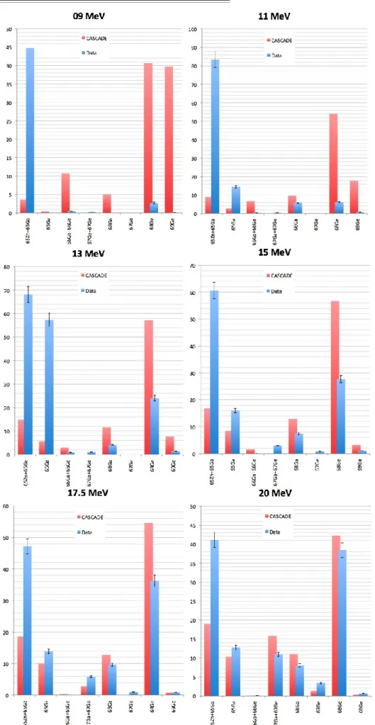
fusion has been obtained comparing the experimental ER production relative cross-sections with the predictions of the statistical code CASCADE. The relative production yelds measured at different energies have been compared with the same quantity obtained by CASCADE. In figures 4.10 and 4.11 such comparison is shown in the case of the 6Li and 7Li projectiles respectively.

The comparisons for the 6Li+64Zn collision shows an interesting behavior: at bombarding energies well above the Coulomb barrier (Vb ≈ 13 MeV) the overall comparison shows that CF is still dominant but a non negligible extra yield with respect to the CF cascade calculations is observed for the sum of 65Zn and 65Ga. Such ER can be both produced in deuteron-ICF, where the alpha particle escapes away; moreover the 65Zn isotope can be also produced in neutron transfer reactions. As the bombarding energy is decreasing CASCADE predicts a larger heavy ER production (less excitation energy leads to less evaporation) but data are showing the opposite behavior, with a strong contribution of 65Ga and 65Zn dominating the relative yield of heavy ERs.

The comparison for the preliminary data of the 7Li+64Zn collision at energies well above the Coulomb barrier shows, although less evidently, an extra yield with respect to the CF cascade calculations for the sum of 65Zn and 65Ga isotopes. Both ER can be also produced by tritium ICF. At sub-barrier energies the ER distribution is dominated by lighter masses showing a dominant ICF contribution.

In conclusions, for both systems the ICF contribution appears to be not negligible and becomes dominant when the bombarding energy decrease below the Coulomb barrier.

Fig. 4.10 a: Production relative yields for the 6Li+64Zn collision compared with the statistical model calculations (CASCADE)

Fig. 4.10 b: Production relative yields for the 6_Li+64_{Zn collision compared with the} statistical model calculations (CASCADE)

Fig. 4.11 a: Production relative yields for the 7Li+64Zn collision compared with the statistical model calculations (CASCADE)

Fig. 4.11 b: Production relative yields for the 7_Li+64_{Zn collision compared with the} statistical model calculations (CASCADE)

4.7 Total fusion and total reaction cross-sections

The fusion cross-section has been extracted as the sum of the ERs production cross-sections paying attention to not consider twice the contribution of father nuclei, which are also detected in their daughter nuclei activity. The total fusion cross-section indetermination is due to geometrical efficiency error (see paragraph 3.3) and fit parameters errors (see paragraph 4.3). In figure 4.12 are shown the total reaction cross-section measured by the elastic scattering in chapter 2, and the fusion cross-section for the 6Li+64Zn system. Data from Gomes et al. [13] are also shown in order to make a comparison. The total reaction cross-section agrees with the existing data of Gomes et al. [13] whereas the total fusion cross-section appears to be larger than previously published data [13]. This appears to confirm the presence of possible experimental problems in the 6_Li+64_{Zn fusion data of [13] as suggested by the same authors in [14]. Similarly the total} reaction and total fusion cross-sections for the 7Li+64Zn system are shown in figure 4.13.

Fig. 4.12: Total fusion cross-section and total reaction cross-section

compared with the ones measured by Gomes et al. for the 6_Li+64_{Zn system.} The total reaction cross-section (red triangles) agrees with the existing data of Gomes et al. [13] (yellow squares) whereas the total fusion cross-section (blue diamonds) appears to be larger than previously published data [13] (red dots).

Fig. 4.13: Total fusion cross-section (blue diamonds) and total reaction

cross-section (red triangles) compared with the ones measured by Gomes et al. for the 7_Li+64_{Zn system. The total reaction cross-section (red triangles)} agrees with the existing data of Gomes et al. [13] (yellow squares) and the total fusion cross-section (blue diamonds) agrees with previously published data [13] (red circles).

As already discussed in paragraph 1.9.1 one of the goals of the performed experiments was to compare the total fusion excitation functions for the 6,7Li+64Zn systems in order to look for possible effects due to the different structure of the two weakly bound projectiles. In figure 4.14 is shown the ratio between the total fusion excitation function for the 6Li+64Zn system and the 7Li+64Zn one as measured by Beck et al. [12] for the 6,7Li+59Co systems (see figure 1.32). Data on 6,7Li+64Zn systems seems to confirm the behavior observed for the 6,7Li+59Co systems. Additional calculations such as the CDCC prediction for fusion cross-section have still to be performed in order to understand the observed enhancement.

Fig. 4.14: Ratio between the 6_Li+64_{Zn and} 7_Li+64_{Zn total fusion} cross-sections. The upper-right picture is figure 1.32, here shown to evidence the similar trend observed for the 6,7_Li+59_{Co fusion data of ref [12]. The solid} line is a guide for the eye.